
12.2.1 Nonlinear Resonator
Analog filters used in music technology are not strictly speaking linear, because at high signal levels they produce distortion. One attempt to include this phenomenon in digital filters has been described by Rossum [Ros92]. He proposed inserting a saturating nonlinearity in the feedback path of a second-order all-pole filter, see Figure 12.1. In this case, the clipper is a symmetrical hard limiter. With this modification, the filter behaves a lot like an analog filter. It produces harmonic distortion and compression when the input signal level is high. Furthermore, its resonance frequency changes when the filter is overloaded, as pointed out in [Ros92]. This technique was used in the E-mu EMAX II sampler, which appeared in 1989. It is an early example of a virtual analog filter used in commercial products.
Figure 12.1 A digital resonant filter with a nonlinear element in its feedback path [Ros92].
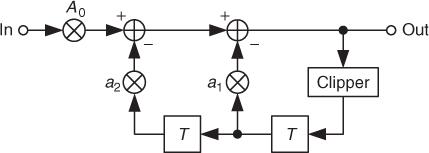
A MATLAB® implementation of Rossum's nonlinear resonator is given in M-file 12.1. The filter coefficients A0, a1, and a2 are computed as in a conventional digital resonator, see, e.g., [Ste96]. In the following examples, we set the resonance frequency to 1 kHz and the bandwidth to 20 Hz. The sampling rate is fS = 44.1 kHz. The saturation limit of the clipper is set to 1.0.
M-file 12.1 (nlreson.m)
function y = nlreson(fc, bw, limit, x)
% function y = nlreson(fc, bw, limit, x)
% Authors: Välimäki, Bilbao, Smith, Abel, Pakarinen, Berners
%
% Parameters:
% fc = center frequency (in Hz)
% bw = bandwidth of resonance (in Hz)
% limit = saturation level
% x = input signal
fs = 44100; % Sampling rate
R = 1 - pi*(bw/fs); % Calculate pole radius
costheta = ((1+(R*R))/(2*R))*cos(2*pi*(fc/fs)); % Cosine of pole angle
a1 = -2*R*costheta; % Calculate first filter coefficient
a2 = R*R; % Calculate second filter coefficient
A0 = (1 - R*R)*sin(2*pi*(fc/fs)); % Scale factor
y = zeros(size(x)); % Allocate memory for output signal
w1 = 0; w2 = 0; % Initialize state variables (unit delays)
y(1) = A0*x(1); % The first input sample goes right through
w0 = y(1); % Input to the saturating nonlinearity
for n = 2:length(x); % Process the rest of input samples
if y(n-1) > limit, w0 = limit; % Saturate above limit
elseif y(n-1) < -limit, w0 = - limit; % Saturate below limit
else w0 = y(n-1);end % Otherwise do nothing
w2 = w1; % Update the second state variable
w1 = w0; % Update the first state variable
y(n) = A0*x(n) - a1*w1 - a2*w2; % Compute filter output
end
When the amplitude of the input signal is 1.0, no distortion occurs, because the signal level at the input of the first state variable (unit delay) does not exceed the saturation level. However, when the input amplitude is larger than the saturation limit, the filter compresses and distorts the signal. At the same time aliasing occurs, since all distortion components above the Nyquist limit get mirrored back to the audio band. To avoid this, it would be necessary run the filter at a higher sample rate.
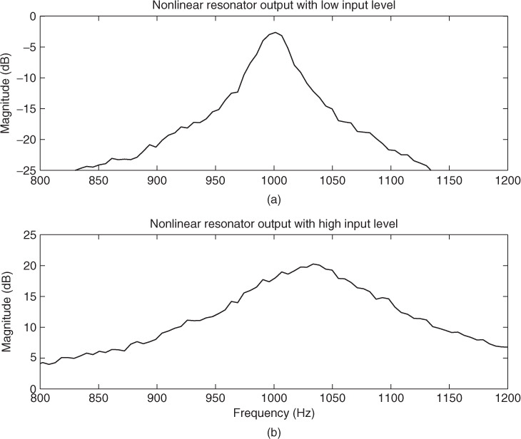
Figure 12.2 shows two examples of the power spectrum of the output signal of the nonlinear resonator, when the input signal is a white-noise sequence. In Figure 12.2(a) the random samples are uniformly distributed between −1.0 and 1.0, while in Figure 11.2(b) they are distributed between −40 and 40. Again, the limit has been set to 1.0. In Figure 12.2(a) the peak in the power spectrum appears at 1000 Hz, as expected, and the −3 dB bandwidth is 20 Hz. However, in Figure 12.2(b), the center frequency has changed: It is now about 1030 Hz. Additionally, the bandwidth is wider than before, about 70 Hz. These phenomena are caused by the saturating nonlinear element, as explained in [Ros92].
Figure 12.2 Power spectrum of the output signal when the input signal is (a) a low-level and (b) a high-level white-noise sequence.
12.2.2 Linear and Nonlinear Digital Models of the Moog Ladder Filter
Next we discuss a well-known analog filter originally proposed by Robert Moog for his synthesizer designs [Moo65]. The filter consists of four one-pole filters in cascade and a global negative feedback loop. The structure is called a ladder filter because of the way in which the one-pole filter sections are cascaded. The filter includes a feedback gain factor k, which may be varied between 0 and 4. This unusual choice of range comes from the fact that at the cut-off frequency the gain of each filter section is 1/4. When k = 4.0, the Moog filter oscillates at its cut-off frequency (i.e., self-oscillates). The Moog ladder filter is also famous for its uncoupled control of the resonance (Q value) and the corner frequency, which are directly adjusted by the feedback gain k and the cut-off frequency parameters, respectively.
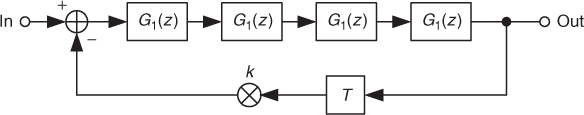
Stilson and Smith [SS96] have considered various methods of converting the Moog ladder filter into a corresponding digital filter. They found that standard transforms, the bilinear and the backward difference transform, yield a structure containing a delay-free path from input to output. To solve this problem, an ad-hoc unit delay may be inserted into the feedback loop. Figure 12.3 shows the resulting filter structure with the extra unit delay. Since the one-pole filters remain first-order filters in the digital implementation, but there is now an extra unit delay, the overall system becomes a fifth-order filter.
Figure 12.3 The digital Moog filter structure proposed in [SS96].
Another complication in the discretization of the Moog filter is that the constant-Q control of the corner frequency is lost. This happens with both the bilinear and the backward difference transform, which place the zeros of the first-order filter at different locations. Stilson and Smith have found a useful compromise first-order filter that has largely independent control of the Q value with corner frequency:
12.1 ![]()
where 0 ≤ p ≤ 1 is the pole location. It can be determined conveniently from the normalized cut-off frequency fc (in Hz),
12.2 ![]()
However, this relation is accurate only when the cut-off frequency is not very high (below 2 kHz or so), and otherwise the actual corner frequency of the filter will be higher than expected. A fourth-order polynomial correction to the pole location has been presented in [VH06]. The Q value of the digital Moog filter proposed by Stilson and Smith [SS96] also deviates slightly from constant at large Q values, but this error may be negligible, since humans are not very sensitive to variations in Q [SS96].
Several alternative versions of the digital Moog filter have been proposed over the years. Wise has shown that a cascade of digital allpass filters can be used to realize a filter with a similar behavior [Wis98]. Fontana has derived a simulation of the Moog filter, which avoids the extra delay in the feedback loop [Fon07]. Instead, Fontana directly solves the contribution of the states of first-order lowpass filters to the output signal. This algorithm requires more operations than the version that was described above, because divisions are involved. However, it is likely to be a more faithful simulation of the Moog ladder filter, since the structure is in principle identical to the analog prototype system.
Other researchers have considered the nonlinear behavior of the Moog filter. It is well known that the transistors used in analog filters softly saturate the signal, when the signal level becomes high. Huovilainen [Huo04] first derived a physically correct nonlinear model for the Moog filter, including the nonlinear behavior of all transistors involved. The model contains five instantaneous nonlinear functions in a feedback loop, one for each first-order section and one for the feedback. It was then found that oversampling by a factor of two at least is necessary to reduce aliasing when nonlinear functions are used [Huo04]. The structure self-oscillates when the feedback gain is 1.0. The feedback gain can even be larger than that; the nonlinear functions prevent the system from becoming unstable. The nonlinear functions also provide amplitude compression, because large signal values are limited by each of them.
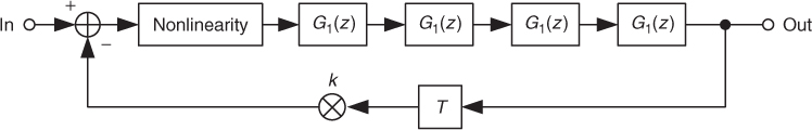
Figure 12.4 shows a simplified version of Huovilainen's nonlinear Moog filter model, in which only one nonlinear function is used [VH06]. The ideal form of the nonlinear function in this case is the hyperbolic tangent function [Huo04]. In real-time implementations this would usually be implemented using a look-up table. Alternatively, another similar smoothly saturating function, such as a third-order polynomial, can be used instead. A MATLAB implementation of the simplified nonlinear Moog filter is given in M-file 12.2.
Figure 12.4 A simplified nonlinear Moog filter structure proposed in [VH06].
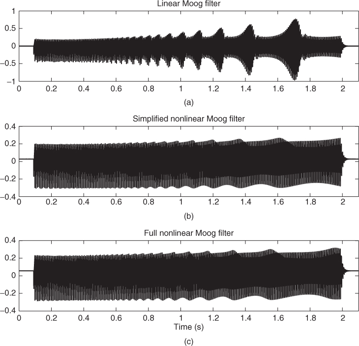
The simplified nonlinear Moog filter may sound slightly different from the full model. However, they share many common features, such as the ability to self-oscillate (when the resonance parameter is set to a value larger than 1) and similar compression characteristics. The latter feature is demonstrated in Figure 12.5, in which a so-called overtone sweep has been generated by filtering a sawtooth signal using three different digital versions of the Moog filter (the signals were published in the Computer Music Journal DVD in 2006 as demonstrations related to [VH06]). The resonant frequency of the filters slowly decreases with time. In Figure 12.5(a), the signal level increases every time the resonance frequency coincides with one of the harmonics of the signal. However, the nonlinear compression decreases these amplitude variations in Figures 12.5(b) and (c). There are minor differences between the two signals, but the output signal envelopes of the two nonlinear models are fairly similar.
M-file 12.2 (moogvcf.m)
function [out,out2,in2,g,h0,h1] = moogvcf(in,fc,res)
% function [out,out2,in2,g,h0,h1] = moogvcf(in,fc,res)
% Authors: Välimäki, Bilbao, Smith, Abel, Pakarinen, Berners
% Parameters:
% in = input signal
% fc= cutoff frequency (Hz)
% res = resonance (0...1 or larger for self-oscillation)
fs = 44100; % Input and output sampling rate
fs2 = 2*fs; % Internal sampling rate
% Two times oversampled input signal:
in = in(:); in2 = zeros(1,2*length(in)); in2(1:2:end) = in;
h = fir1(10,0.5); in2 = filter(h,1,in2); % Anti-imaging filter
Gcomp = 0.5; % Compensation of passband gain
g = 2*pi*fc/fs2; % IIR feedback coefficient at fs2
Gres = res; % Direct mapping (no table or polynomial)
h0 = g/1.3; h1 = g*0.3/1.3; % FIR part with gain g
w = [0 0 0 0 0]; % Five state variables
wold = [0 0 0 0 0]; % Previous states (unit delays)
out = zeros(size(in)); out2 = zeros(size(in2));
for n = 1:length(in2),
u = in2(n) - 4*Gres*(wold(5) - Gcomp*in2(n)); % Input and feedback
w(1) = tanh(u); % Saturating nonlinearity
w(2) = h0*w(1) + h1*wold(1) + (1-g)*wold(2); % First IIR1
w(3) = h0*w(2) + h1*wold(2) + (1-g)*wold(3); % Second IIR1
w(4) = h0*w(3) + h1*wold(3) + (1-g)*wold(4); % Third IIR1
w(5) = h0*w(4) + h1*wold(4) + (1-g)*wold(5); % Fourth IIR1
out2(n) = w(5); % Filter output
wold = w; % Data move (unit delays)
end
out2 = filter(h,1,out2); % Antialiasing filter at fs2
out = out2(1:2:end); % Decimation by factor 2 (return to original fs)
Figure 12.5 Sawtooth signal filtered with three Moog filter models: (a) the linear Stilson—Smith model of Figure 12.3, (b) the simplified nonlinear model of Figure 12.4, and (c) the full nonlinear model [Huo04].
12.2.3 Tone Stack
As another useful example of a virtual analog filter, a three-channel equalizing filter used in electric guitar and bass amplifiers is presented. This so-called tone stack has the following linear third-order transfer function,
12.3 ![]()
Yeh has derived the parameter values for this digital tone stack model [YS06, Yeh09]. The equations can be seen in the M-file 12.3 below. Three parameters (top, mid, and low), which all affect several filter coefficients, can be varied to adjust the filter's magnitude response.
M-file 12.3 (bassman.m)
function [y,B0,B1,B2,B3,A0,A1,A2,A3] = bassman(low, mid, top, x)
% function [y,B0,B1,B2,B3,A0,A1,A2,A3] = bassman(low, mid, top, x)
% Authors: Välimäki, Bilbao, Smith, Abel, Pakarinen, Berners
%
% Parameters:
% low = bass level
% mid = noise level
% top = treble level
% x = input signal
fs = 44100; % Sample rate
C1 = 0.25*10∧-9;C2 = 20*10∧-9;C3 = 20*10∧-9; % Component values
R1 = 250000;R2 = 1000000;R3 = 25000;R4 = 56000; % Component values
% Analog transfer function coefficients:
b1 = top*C1*R1 + mid*C3*R3 + low*(C1*R2 + C2*R2) + (C1*R3 + C2*R3);
b2 = top*(C1*C2*R1*R4 + C1*C3*R1*R4) - mid∧2*(C1*C3*R3∧2 + C2*C3*R3∧2) ...
+ mid*(C1*C3*R1*R3 + C1*C3*R3∧2 + C2*C3*R3∧2) ...
+ low*(C1*C2*R1*R2 + C1*C2*R2*R4 + C1*C3*R2*R4) ...
+ low*mid*(C1*C3*R2*R3 + C2*C3*R2*R3) ...
+ (C1*C2*R1*R3 + C1*C2*R3*R4 + C1*C3*R3*R4);
b3 = low*mid*(C1*C2*C3*R1*R2*R3 + C1*C2*C3*R2*R3*R4) ...
- mid∧2*(C1*C2*C3*R1*R3∧2 + C1*C2*C3*R3∧2*R4) ...
+ mid*(C1*C2*C3*R1*R3∧2 + C1*C2*C3*R3∧2*R4) ...
+ top*C1*C2*C3*R1*R3*R4 - top*mid*C1*C2*C3*R1*R3*R4 ...
+ top*low*C1*C2*C3*R1*R2*R4;
a0 = 1;
a1 = (C1*R1 + C1*R3 + C2*R3 + C2*R4 + C3*R4) + mid*C3*R3 ...
+ low*(C1*R2 + C2*R2);
a2 = mid*(C1*C3*R1*R3 - C2*C3*R3*R4 + C1*C3*R3∧2 + C2*C3*R3∧2) ...
+ low*mid*(C1*C3*R2*R3 + C2*C3*R2*R3) ...
- mid∧2*(C1*C3*R3∧2 + C2*C3*R3∧2) ...
+ low*(C1*C2*R2*R4 + C1*C2*R1*R2 + C1*C3*R2*R4 + C2*C3*R2*R4) ...
+ (C1*C2*R1*R4 + C1*C3*R1*R4 + C1*C2*R3*R4 + C1*C2*R1*R3 ...
+ C1*C3*R3*R4 + C2*C3*R3*R4);
a3 = low*mid*(C1*C2*C3*R1*R2*R3 + C1*C2*C3*R2*R3*R4) ...
- mid∧2*(C1*C2*C3*R1*R3∧2 + C1*C2*C3*R3∧2*R4) ...
+ mid*(C1*C2*C3*R3∧2*R4 + C1*C2*C3*R1*R3∧2 ...
- C1*C2*C3*R1*R3*R4) + low*C1*C2*C3*R1*R2*R4 + C1*C2*C3*R1*R3*R4;
% Digital filter coefficients:
c = 2*fs;
B0 = -b1*c - b2*c∧2 - b3*c∧3; B1 = -b1*c + b2*c∧2 + 3*b3*c∧3;
B2 = b1*c + b2*c∧2 - 3*b3*c∧3; B3 = b1*c - b2*c∧2 + b3*c∧3;
A0 = -a0 - a1*c - a2*c∧2 - a3*c∧3;
A1 = -3*a0 - a1*c + a2*c∧2 + 3*a3*c∧3;
A2 = -3*a0 + a1*c + a2*c∧2 - 3*a3*c∧3;
A3 = -a0 + a1*c - a2*c∧2 + a3*c∧3;
y = filter(B,A,x); % Output signal
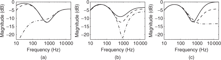
Figure 12.6 shows examples of magnitude responses with different parameter settings. Figure 12.6(a), (b), and (c) present the variations in the low-, middle-, and high-frequency regions, respectively. Note that the parameters are not strictly independent, but they all affect the filter gain in the middle range (see, for example, the magnitude response around 1 kHz). Furthermore, the neutral setting (low = mid = top = 0.5) does not yield a flat response, see dashed lines in Figure 12.6. This filter has its own character.
Figure 12.6 Magnitude responses of the tone stack filter model with the following parameters: (a) low = 0 (dash-dot line), low = 0.5 (dashed line), low = 1 (solid line), (b) mid = 0 (dash-dot line), mid = 0.5 (dashed line), mid = 1 (solid line), (c) top = 0 (dash-dot line), top = 0.5 (dashed line), top = 1 (solid line). The rest of the parameters are set to 0.5 in each case.
12.2.4 Wah-wah Filter
The wah-wah filter was introduced in Section 2.4.1. It operates by sweeping a single resonance through the spectrum. Typically this resonance is second-order. Following [Smi08], this section will describe digitization of the “CryBaby” wah-wah filter controlled by footpedal.
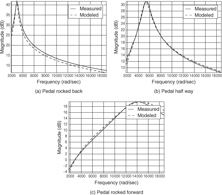
Figure 12.7(a), (b), and (c) show the amplitude responses (solid lines) of a CryBaby wah pedal measured at three representative pedal settings (rocked fully backward, middle, and forward). Our goal is to “digitize” the CryBaby by devising a sweeping resonator that audibly matches these three responses when the “wah” variable is 0, 1/2, and 1, respectively. The results of this exercise are shown in dashed lines in 12.7(a)–(c), and the audible quality is excellent.
Figure 12.7 Measured (solid) and modeled (dashed) amplitude responses of the CryBaby wah pedal at three different pedal angles [Smi08].
Based on the measured shape of the amplitude response (a bandpass-resonator characteristic), and knowledge (from circuit schematics) that the bandpass is second-order, the transfer function can be presumed to be of the form
12.4 
where g is an overall gain factor, ξ is a real zero at or near dc (the other being at infinity), ωr is the pole resonance frequency, and Q is the so-called “quality factor” of the resonator [Smi07].1 The measurements reveal that ωr, Q, and g all vary significantly with pedal angle θ. As discussed in [Smi08], good choices for these functions are as shown in M-file 12.4, where the controlling wah variable is the pedal-angle θ normalized to a [0, 1] range.
M-file 12.4 (wahcontrols.m)
function [g,fr,Q] = wahcontrols(wah)
% Authors: Välimäki, Bilbao, Smith, Abel, Pakarinen, Berners
% function [g,fr,Q] = wahcontrols(wah)
%
% Parameter: wah = wah-pedal-angle normalized to lie between 0 and 1
g = 0.1*4∧wah; % overall gain for second-order s-plane transfer funct.
fr = 450*2∧(2.3*wah); % resonance frequency (Hz) for the same transfer funct.
Q = 2∧(2*(1-wah)+1); % resonance quality factor for the same transfer funct.
Digitization
Closed-form expressions for digital filter coefficients in terms of (Q,fr,g) based on z = est ≈ 1 + sT (low-frequency resonance assumed) yield the code shown in M-file 12.5.
M-file 12.5 (wahdig.m)
% wahdig.m
% Authors: Välimäki, Bilbao, Smith, Abel, Pakarinen, Berners
% A = wahdig(fr,Q,fs)
%
% Parameters:
% fr = resonance frequency (Hz)
% Q = resonance quality factor
% fs = sampling frequency (Hz)
%
% Returned:
% A = [1 a1 a2] = digital filter transfer-function denominator poly
frn = fr/fs;
R = 1 - PI*frn/Q; % pole radius
theta = 2*PI*frn; % pole angle
a1 = -2.0*R*cos(theta); % biquad coeff
a2 = R*R; % biquad coeff
Note that in practice each time-varying coefficient should be smoothed, e.g., by a unity-gain one-pole smoother with pole at p = 0.999:
12.5 ![]()
Virtual CryBaby Results
While the presented wah pedal model sounds very faithful to the original (minus its noise), at low resonance frequencies the loudness is significantly greater than at high resonance frequencies. (This is a characteristic of the original wah pedal.) Therefore, an improvement over the original could be to determine a new scaling function g(wah) that preserves constant loudness as much as possible as the pedal varies. A similar effect can be had by applying dynamic range compression to the wah output, as is often done when recording an electric guitar.
A Faust2 software implementation of the CryBaby wah pedal described in this section is included in the Faust distribution (file effect.lib).
12.2.5 Phaser
The phasing effect was introduced in Section 2.4.2. It operates by sweeping a few “notches” through the input signal spectrum. The notches are created by summing the input signal with a variably phase-shifted version of the input signal, as shown in Figure 12.8. The phase-shifting stages are conventionally first- or second-order allpass filters [Smi07].3
Figure 12.8 Phaser implemented by summing the direct signal with the output of four first-order allpass filters in series (from [Smi10]).
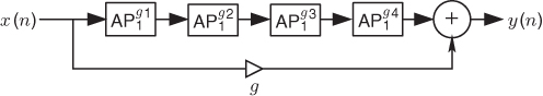
In analog hardware, such as the Univibe or MXR phase shifters, the allpass filters are typically first-order. Thus, each analog allpass has a transfer function of the form
where we will call ωb (a real number) the break frequency of the allpass.
To create a virtual analog phaser, following closely the design of typical analog phasers, we must translate each first-order allpass to the digital domain. In discrete time, the general first-order allpass has the transfer function
12.7 ![]()
Thus, we wish to “digitize” each first-order allpass by means of a mapping from the s plane to the z plane. There are several ways to accomplish this goal [RG75]. In this case, an excellent choice is the bilinear transformation4 defined by
where c is chosen to map one particular analog frequency to a particular digital frequency (other than dc or half the sampling rate, which are always mapped from dc and infinity in the s plane, respectively). In this case, c is well chosen for each section to map the break frequency of the section to the corresponding point on the digital frequency axis. The relation between analog frequency ωa and digital frequency ωd follows immediately from Equation (12.8):
Thus, given a particular desired break-frequency ωa = ωd = ωb, we can set
12.10 ![]()
The bilinear transform preserves filter order (so we will obtain a first-order digital allpass for each first-order analog allpass), and it always maps a stable analog filter to a stable digital filter. In fact, the entire jω axis of the s plane maps to the unit circle of the z plane, giving a one-to-one correspondence between the analog and digital frequency axes. The main error in the bilinear transform is its frequency warping, which is displayed in Equation (12.9). Only dc and one other finite frequency (chosen by setting c) are mapped without any warping error.
Applying the bilinear transformation Equation (12.8) to the first-order analog allpass filter Equation (12.6) gives
12.11 
where we have denoted the pole of the digital allpass by
12.12 ![]()
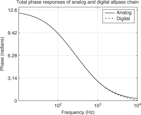
Figure 12.9 shows the digital phaser response curves. They look almost identical to the analog response curves. While the break frequencies are preserved by construction, the notches have moved slightly, although this is not visible from the plots. An overlay of the total phase of the analog and digital allpass chains is shown in Figure 12.10. We can see that the phase responses of the analog and digital allpass chains diverge visibly only above 9 kHz. The analog phase response approaches zero in the limit as ωa → ∞, while the digital phase response reaches zero at half the sampling rate, 10 kHz in this case. This is a good example of when the bilinear transform performs very well to digitize an analog system.
Figure 12.9 (a) Phase responses of first-order digital allpass sections having break frequencies at 100, 200, 400, and 800 Hz. The sampling rate is 20 kHz. (b) Corresponding phaser amplitude response [Smi10].
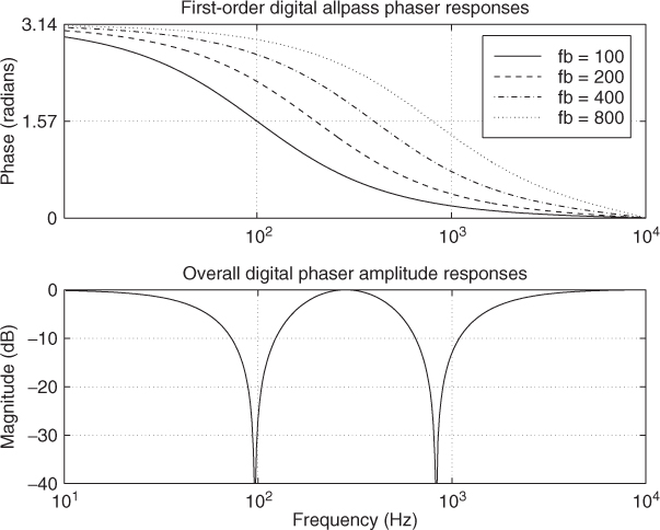
Figure 12.10 Phase response of four first-order allpass sections in series—analog and digital cases overlaid [Smi10].
In general, the bilinear transform works well to digitize feedforward analog structures in which the high-frequency warping is acceptable. When frequency warping is excessive, it can be alleviated by the use of oversampling; for example, the slight visible deviation in Figure 12.10 below 10 kHz can be largely eliminated by increasing the sampling rate by 15% or so. See digitizing the Moog VCF for an example in which the presence of feedback in the analog circuit leads to a delay-free loop in the digitized system under the bilinear transform [SS96, Sti06]. In such cases it is common to insert an extra unit delay in the loop, which has little effect at low frequencies. See Section 12.2.2. (Stability should then be carefully checked, as it is no longer guaranteed.)
Phasing with Second-order Allpass Filters
While the use of first-order allpass sections is classic for hardware phase shifters, second-order allpass filters, mentioned in Section 2.4.2, are easier to use for generating precisely located notches that are more independently controllable [Smi84].
The architecture of a phaser based on second-order allpasses is identical to that in Figure 12.8, but with each first-order allpass ![]() being replaced by a second-order allpass
being replaced by a second-order allpass ![]() , where the control parameters Ri and θi are given below. As before, the phaser will have a notch wherever the phase of the allpass chain passes through π radians (180 degrees). It can be shown that for second-order allpasses notch frequencies occur close to the resonant frequencies of the allpass sections [Smi84]. It is therefore convenient to use allpass sections of the form
, where the control parameters Ri and θi are given below. As before, the phaser will have a notch wherever the phase of the allpass chain passes through π radians (180 degrees). It can be shown that for second-order allpasses notch frequencies occur close to the resonant frequencies of the allpass sections [Smi84]. It is therefore convenient to use allpass sections of the form
12.13 ![]()
where
![]()