
Chapter 9
Mixture Design
The good things of life are not to be had singly, but come to us with a mixture.
Charles Lamb
The cliché image of experimentation is a crazed person in a lab coat pouring fluorescent liquids into bubbling beakers. Ironically, the standard approaches for design of experiments (DOE) don’t work very well on experiments that involve mixtures. The following illustration shows why.
For example, what would happen if you performed a factorial design on combinations of lemonade and apple juice? Table 9.1 shows the experimental layout with two levels of each factor—either one or two cups.
Factorial design on mixture of fruit juices
|
Std Order |
A: Lemonade (cups) |
B: Apple juice (cups) |
Ratio |
|
1 |
1 |
1 |
1/1 |
|
2 |
2 |
1 |
2/1 |
|
3 |
1 |
2 |
1/2 |
|
4 |
2 |
2 |
1/1 |
Notice that standard orders 1 and 4 call for mixtures with the same ratio of lemonade to apple juice. The total amount varies, but will have no effect on responses, such as taste, color, or viscosity. Therefore, it makes no sense to do the complete design. When responses depend only on proportions and not the amount of ingredients, factorial designs don’t work very well.
Another approach to this problem is to take the amount variable out of the experiment and work on a percentage basis. Table 9.2 shows the layout for a second attempt at the juice experiment, with each “component” at two levels: 0 or 100%.
Alternative factorial design on fruit juices in terms of percentage
|
Std Order |
A: Lemonade (%) |
B: Apple juice (%) |
Total (%) |
|
1 |
0 |
0 |
0 |
|
2 |
100 |
0 |
100 |
|
3 |
0 |
100 |
100 |
|
4 |
100 |
100 |
200 |
This design, which asks for impossible totals, does not work any better than the first design. It illustrates a second characteristic of mixtures: The total is “constrained” because ingredients must add up to 100%.
Two-Component Mixture Design: Good as Gold
Several thousand years ago, a jewelry maker discovered that adding copper to gold reduces the melt point of the resulting mixture. This led to a breakthrough in goldsmithing, because small decorations could be soldered to a main element of pure gold with a copper-rich alloy. The copper blended in with no noticeable loss of luster in the finished piece.
Table 9.3 lays out a simple mixture experiment aimed at quantifying this metallurgical phenomenon.
A mixture experiment on copper and gold
|
Blend |
A: Gold (wt%) |
B: Copper (wt%) |
Melt Point (deg C) |
|
Pure |
100 |
0 |
1039, 1047 |
|
Binary |
50 |
50 |
918, 922 |
|
Pure |
0 |
100 |
1073, 1074 |
This is a fully replicated design on the pure metals and their binary (50/50) blend. For a proper replication, each blend must be reformulated, not just retested for melt point. If the blends are simply retested for melt point without reformulation, the only variation is due to testing, not the entire process, and error will be underestimated. It is also critical to randomize the run order. Don’t do the same formulation twice in a row, because you will more than likely get results that reflect less than the normal process variation.
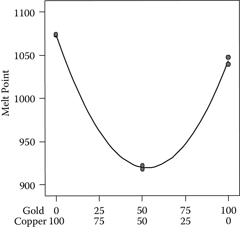
Notice the depression in melt point in the blend. This is desirable and, therefore, an example of “synergistic” behavior. It can be modeled with the following equation:
Melt point = 1043.0 A + 1073.5 B − 553.2 AB
where components A and B are expressed in proportional scale (0 to 1). This second-order “mixture model,” developed by Henri Scheffé, is easy to interpret. The coefficients for the main effects are the responses for the purest “blends” for A and B. The second-order term AB looks like a two-factor interaction, but in the mixture model, it’s referred to as a quadratic, or sometimes nonlinear, blending term. The negative coefficient on AB indicates that a combination of the two components produces a response that is less than what you would expect from linear blending. This unexpected curvature becomes more obvious in the response surface graph shown in Figure 9.1.
This is a highly simplified view of the actual behavior of copper and gold mixtures. To pin it down further, one would need to add a number of check blends to fill in the blanks between these compositions. The predicted value for equal amounts of gold and copper is
Melt point = 1043.0 (0.5) + 1073.5 (0.5) − 553.2 (0.5 * 0.5)
= (1043.0 + 1073.5)/2 − 553.2/4 = 1058.25 − 138.3 = 919.95
The equation predicts a deflection of 138.3°C from the melt point of 1058.25 that one would expect from linear blending; simply the average of the melt points for the two metals. Statistical analysis of the overall model and the interaction itself reveals a significant fit.
Three-Component Design: Teeny Beany Experiment
Formulators usually experiment on more than two components. A good example of this is a mixture design on three flavors of small jelly candies called teeny beanies. Table 9.4 shows the blends and resulting taste ratings. The rating system, similar to the one used for the popcorn experiments in Chapter 3, goes from 1 (worst) to 10 (best). Each blend was rated by a panel, but in a different random order for each taster. The ratings were then averaged. Several of the blends were replicated to provide estimates of pure error.
Teeny beany mixture design (three-component)
|
Blend |
A: Apple % |
B: Cinnamon % |
C: Lemon % |
Taste Rating |
|
Pure |
100.00 |
0.00 |
0.00 |
5.1, 5.2 |
|
Pure |
0.00 |
100.00 |
0.00 |
6.5, 7.0 |
|
Pure |
0.00 |
0.00 |
100.00 |
4.0, 4.5 |
|
Binary |
50.00 |
50.00 |
0.00 |
6.9 |
|
Binary |
50.00 |
0.00 |
50.00 |
2.8 |
|
Binary |
0.00 |
50.00 |
50.00 |
3.5 |
|
Centroid |
33.33 |
33.33 |
33.33 |
4.2, 4.3 |
This design is called a simplex centroid because it includes a blend with equal proportions of all the components. The centroid falls at the center of the mixture space, which forms a simplex—a geometric term for a figure with one more vertex than the number of dimensions. For three components, the simplex is an equilateral triangle. The addition of a fourth component creates a tetrahedron, which looks like a three-sided pyramid. Because only two-dimensional space can be represented on a piece of paper or computer screen, response data for mixtures of three or more components are displayed on triangular graphs such as the one shown in Figure 9.2.

Notice that the grid lines increase in value as you move from any of the three sides toward the opposing vertex. The markings on this graph are in terms of percentage, so each vertex represents 100% of the labeled component. The unique feature of this trilinear graph paper is that only two components need to be specified. At this point, the third component is fixed. For example, the combination of X1 at 33.3% (1/3rd of the way up from the bottom) plus X2 at 33.3% (1/3rd of the distance from the right side to lower left vertex) is all that is required to locate the centroid (shown on the graph). You then can read the value of the remaining component (X3), which must be 33.3% to bring the total to approximately 100%.
Figure 9.3 shows a contour map fitted to the taste responses for the various blends of teeny beanies.

Notice the curves in the contours. This behavior is modeled by the following second-order Scheffé polynomial:
Taste = 5.14 A + 6.74 B + 4.24 C + 4.12 AB − 7.28 AC − 7.68 BC
Analysis of variance (not shown) indicates that this model is highly significant. Component B, cinnamon, exhibits the highest coefficient for the main effects. Thus, one can conclude that the best pure teeny beanie is cinnamon. Component C, lemon, was least preferred. Looking at the coefficients for the second-order terms, you can see by the positive coefficient that only the AB combination (apple–cinnamon) was rated favorably. The tasters gave low ratings to the apple–lemon (AC) and lemon–cinnamon (BC) combinations. These synergisms and antagonisms are manifested by upward and downward curves along the edges of the 3-D response surface shown in Figure 9.4.

This concludes our overview of mixture design, but we have only scratched the surface of this DOE tool geared for chemists of food, pharmaceuticals, coatings, cosmetics, metals, plastics, etc. For more details, see “A Primer on Mixture Design: What’s In It for Formulators?” online at www.statease.com/formulator and study the referenced texts by Cornell or Smith.
Shotgun Approach to Mixture Design
Chemists are famous for creating mysterious concoctions seemingly by magic. A typical example is Hoppe’s Nitro Powder Solvent Number 9, invented by Frank August Hoppe. While fighting in the Spanish–American War, Captain Hoppe found it extremely difficult to ream corrosion from his gun barrel. The problem was aggravated by the antagonistic effects of mixing old black powder with new smokeless powder. After several years of experimenting in his shed, Hoppe came up with a mixture of nine chemicals that worked very effectively. A century or so later, his cleaning solution is still sold. The composition remains a trade secret.
Good Or Bad: Watch Out for Nonlinear Blending
There are two ways that components can unexpectedly combine: positively (synergism) or negatively (antagonism). With synergism, you get a better response than what you would expect to get from simply adding the effects of each ingredient alone. In other words, adding one to one gives you more than two. For example, if you combined two different types of firecrackers and got an explosion like an atomic bomb, you would be the beneficiary (victim?) of synergism. On the other hand, with antagonism, you get a poorer response than what you would expect from the combination of ingredients. As an analogy, one of the authors (Mark) observed antagonism at an early age between his two similarly aged sons, and two similarly aged daughters. These are classic cases of sibling rivalry or, in the parlance of mixture design, negatively nonlinear blending. A child may act very positively on his or her own, but in the presence of a sibling, they compete in a negative way for parental attention. Although antagonism is the norm, siblings can act synergistically, such as when they happily play together. Wouldn’t that be nice?
Worth Its Weight in Gold?
An ancient king suspected that his goldsmith had mixed some silver into a supposedly pure gold crown. He asked the famous mathematician Archimedes to investigate. Archimedes performed the following experiment:
- Create a bar of pure gold with the same weight as the crown.
- Put the gold in a bath tub. Measure the volume of water spilled.
- Do the same with the crown.
- Compare the volumes.
Archimedes knew that silver would be less dense than gold. Therefore, upon finding that the volume of the crown exceeded the volume of an equal weight of gold, he knew that the crown contained silver. According to legend, the naked Archimedes then ran from his bath into the street shouting, “Eureka!” (Greek for “I have found it.”)
The principles of mixture design can be put to work in this case. Gold and silver have densities of 10.2 and 5.5 troy ounces per cubic inch, respectively. Assume that no density interactions exist between silver and gold. We then can apply a linear mixture model to predict weight (in ounces) of one cubic inch (enough to make a crown?) as a function of proportional volume for gold (A) versus silver (B).
Weight = 10.2 A + 5.5 B
Notice that the coefficients of the model are simply the densities of the pure metals. The weight of a blend of half gold and half silver is calculated as follows:
Weight = 10.2 (0.5) + 5.5 (0.5) = 7.85 troy ounces per cubic inch