The Idea

Whenever you look at some source of data, it’s likely that the data will somehow form clusters. A dataset showing where millionaires live probably has clusters in places like Beverly Hills and Manhattan. A dataset showing how many hours people work each week probably has a cluster around 40 (and if it’s taken from a state with laws mandating special benefits for people who work at least 20 hours a week, it probably has another cluster right around 19). A dataset of demographics of registered voters likely forms a variety of clusters (e.g., “soccer moms,” “bored retirees,” “unemployed millennials”) that pollsters and political consultants consider relevant.

Unlike some of the problems we’ve looked at, there is generally no “correct” clustering. An alternative clustering scheme might group some of the “unemployed millennials” with “grad students,” and others with “parents’ basement dwellers.” Neither scheme is necessarily more correct—instead, each is likely more optimal with respect to its own “how good are the clusters?” metric.

Furthermore, the clusters won’t label themselves. You’ll have to do that by looking at the data underlying each one.

The Model

For us, each input will be a vector in d-dimensional space, which, as usual, we will represent as a list of numbers. Our goal will be to identify clusters of similar inputs and (sometimes) to find a representative value for each cluster.

For example, each input could be a numeric vector that represents the title of a blog post, in which case the goal might be to find clusters of similar posts, perhaps in order to understand what our users are blogging about. Or imagine that we have a picture containing thousands of (red, green, blue) colors and that we need to screen-print a 10-color version of it. Clustering can help us choose 10 colors that will minimize the total “color error.”

One of the simplest clustering methods is k-means, in which the number of clusters k is chosen in advance, after which the goal is to partition the inputs into sets $S_1,...,S_k$ in a way that minimizes the total sum of squared distances from each point to the mean of its assigned cluster.

There are a lot of ways to assign n points to k clusters, which means that finding an optimal clustering is a very hard problem. We’ll settle for an iterative algorithm that usually finds a good clustering:

1. Start with a set of k-means, which are points in d-dimensional space.

2. Assign each point to the mean to which it is closest.

3. If no point’s assignment has changed, stop and keep the clusters.

4. If some point’s assignment has changed, recompute the means and return to step 2.

Using the vector_mean function from Chapter 4, it’s pretty simple to create a class that does this.

To start with, we’ll create a helper function that measures how many coordinates two vectors differ in. We’ll use this to track our training progress:

from scratch.linear_algebra import Vector

def num_differences(v1: Vector, v2: Vector) -> int:
    assert len(v1) == len(v2)
    return len([x1 for x1, x2 in zip(v1, v2) if x1 != x2])

assert num_differences([1, 2, 3], [2, 1, 3]) == 2
assert num_differences([1, 2], [1, 2]) == 0

We also need a function that, given some vectors and their assignments to clusters, computes the means of the clusters. It may be the case that some cluster has no points assigned to it. We can’t take the mean of an empty collection, so in that case we’ll just randomly pick one of the points to serve as the “mean” of that cluster:

from typing import List
from scratch.linear_algebra import vector_mean

def cluster_means(k: int,
                  inputs: List[Vector],
                  assignments: List[int]) -> List[Vector]:
    # clusters[i] contains the inputs whose assignment is i
    clusters = [[] for i in range(k)]
    for input, assignment in zip(inputs, assignments):
        clusters[assignment].append(input)

    # if a cluster is empty, just use a random point
    return [vector_mean(cluster) if cluster else random.choice(inputs)
            for cluster in clusters]

And now we’re ready to code up our clusterer. As usual, we’ll use tqdm to track our progress, but here we don’t know how many iterations it will take, so we then use itertools.count, which creates an infinite iterable, and we’ll return out of it when we’re done:

import itertools
import random
import tqdm
from scratch.linear_algebra import squared_distance

class KMeans:
    def __init__(self, k: int) -> None:
        self.k = k                      # number of clusters
        self.means = None

    def classify(self, input: Vector) -> int:
        """return the index of the cluster closest to the input"""
        return min(range(self.k),
                   key=lambda i: squared_distance(input, self.means[i]))

    def train(self, inputs: List[Vector]) -> None:
        # Start with random assignments
        assignments = [random.randrange(self.k) for _ in inputs]

        with tqdm.tqdm(itertools.count()) as t:
            for _ in t:
                # Compute means and find new assignments
                self.means = cluster_means(self.k, inputs, assignments)
                new_assignments = [self.classify(input) for input in inputs]

                # Check how many assignments changed and if we're done
                num_changed = num_differences(assignments, new_assignments)
                if num_changed == 0:
                    return

                # Otherwise keep the new assignments, and compute new means
                assignments = new_assignments
                self.means = cluster_means(self.k, inputs, assignments)
                t.set_description(f"changed: {num_changed} / {len(inputs)}")

Let’s take a look at how this works.

Example: Meetups

To celebrate DataSciencester’s growth, your VP of User Rewards wants to organize several in-person meetups for your hometown users, complete with beer, pizza, and DataSciencester t-shirts. You know the locations of all your local users (Figure 20-1), and she’d like you to choose meetup locations that make it convenient for everyone to attend.

Figure 20-1. The locations of your hometown users

Depending on how you look at it, you probably see two or three clusters. (It’s easy to do visually because the data is only two-dimensional. With more dimensions, it would be a lot harder to eyeball.)

Imagine first that she has enough budget for three meetups. You go to your computer and try this:

random.seed(12)                   # so you get the same results as me
clusterer = KMeans(k=3)
clusterer.train(inputs)
means = sorted(clusterer.means)   # sort for the unit test

assert len(means) == 3

# Check that the means are close to what we expect
assert squared_distance(means[0], [-44, 5]) < 1
assert squared_distance(means[1], [-16, -10]) < 1
assert squared_distance(means[2], [18, 20]) < 1

You find three clusters centered at [–44, 5], [–16, –10], and [18, 20], and you look for meetup venues near those locations (Figure 20-2).

Figure 20-2. User locations grouped into three clusters

You show your results to the VP, who informs you that now she only has enough budgeted for two meetups.

“No problem,” you say:

random.seed(0)
clusterer = KMeans(k=2)
clusterer.train(inputs)
means = sorted(clusterer.means)

assert len(means) == 2
assert squared_distance(means[0], [-26, -5]) < 1
assert squared_distance(means[1], [18, 20]) < 1

As shown in Figure 20-3, one meetup should still be near [18, 20], but now the other should be near [–26, –5].

Figure 20-3. User locations grouped into two clusters

Choosing k

In the previous example, the choice of k was driven by factors outside of our control. In general, this won’t be the case. There are various ways to choose a k. One that’s reasonably easy to understand involves plotting the sum of squared errors (between each point and the mean of its cluster) as a function of k and looking at where the graph “bends”:

from matplotlib import pyplot as plt

def squared_clustering_errors(inputs: List[Vector], k: int) -> float:
    """finds the total squared error from k-means clustering the inputs"""
    clusterer = KMeans(k)
    clusterer.train(inputs)
    means = clusterer.means
    assignments = [clusterer.classify(input) for input in inputs]

    return sum(squared_distance(input, means[cluster])
               for input, cluster in zip(inputs, assignments))

which we can apply to our previous example:

# now plot from 1 up to len(inputs) clusters

ks = range(1, len(inputs) + 1)
errors = [squared_clustering_errors(inputs, k) for k in ks]

plt.plot(ks, errors)
plt.xticks(ks)
plt.xlabel("k")
plt.ylabel("total squared error")
plt.title("Total Error vs. # of Clusters")
plt.show()

Looking at Figure 20-4, this method agrees with our original eyeballing that three is the “right” number of clusters.

Figure 20-4. Choosing a k

Example: Clustering Colors

The VP of Swag has designed attractive DataSciencester stickers that he’d like you to hand out at meetups. Unfortunately, your sticker printer can print at most five colors per sticker. And since the VP of Art is on sabbatical, the VP of Swag asks if there’s some way you can take his design and modify it so that it contains only five colors.

Computer images can be represented as two-dimensional arrays of pixels, where each pixel is itself a three-dimensional vector (red, green, blue) indicating its color.

Creating a five-color version of the image, then, entails:

1. Choosing five colors.

2. Assigning one of those colors to each pixel.

It turns out this is a great task for k-means clustering, which can partition the pixels into five clusters in red-green-blue space. If we then recolor the pixels in each cluster to the mean color, we’re done.

To start with, we’ll need a way to load an image into Python. We can do this with matplotlib, if we first install the pillow library:

python -m pip install pillow

Then we can just use matplotlib.image.imread:

image_path = r"girl_with_book.jpg"    # wherever your image is
import matplotlib.image as mpimg
img = mpimg.imread(image_path) / 256  # rescale to between 0 and 1

Behind the scenes img is a NumPy array, but for our purposes, we can treat it as a list of lists of lists.

img[i][j] is the pixel in the ith row and jth column, and each pixel is a list [red, green, blue] of numbers between 0 and 1 indicating the color of that pixel:

top_row = img[0]
top_left_pixel = top_row[0]
red, green, blue = top_left_pixel

In particular, we can get a flattened list of all the pixels as:

# .tolist() converts a NumPy array to a Python list
pixels = [pixel.tolist() for row in img for pixel in row]

and then feed them to our clusterer:

clusterer = KMeans(5)
clusterer.train(pixels)   # this might take a while

Once it finishes, we just construct a new image with the same format:

def recolor(pixel: Vector) -> Vector:
    cluster = clusterer.classify(pixel)        # index of the closest cluster
    return clusterer.means[cluster]            # mean of the closest cluster

new_img = [[recolor(pixel) for pixel in row]   # recolor this row of pixels
           for row in img]                     # for each row in the image

and display it, using plt.imshow:

plt.imshow(new_img)
plt.axis('off')
plt.show()

It is difficult to show color results in a black-and-white book, but Figure 20-5 shows grayscale versions of a full-color picture and the output of using this process to reduce it to five colors.

Figure 20-5. Original picture and its 5-means decoloring

Bottom-Up Hierarchical Clustering

An alternative approach to clustering is to “grow” clusters from the bottom up. We can do this in the following way:

1. Make each input its own cluster of one.

2. As long as there are multiple clusters remaining, find the two closest clusters and merge them.

At the end, we’ll have one giant cluster containing all the inputs. If we keep track of the merge order, we can re-create any number of clusters by unmerging. For example, if we want three clusters, we can just undo the last two merges.

We’ll use a really simple representation of clusters. Our values will live in leaf clusters, which we will represent as NamedTuples:

from typing import NamedTuple, Union

class Leaf(NamedTuple):
    value: Vector

leaf1 = Leaf([10,  20])
leaf2 = Leaf([30, -15])

We’ll use these to grow merged clusters, which we will also represent as NamedTuples:

class Merged(NamedTuple):
    children: tuple
    order: int

merged = Merged((leaf1, leaf2), order=1)

Cluster = Union[Leaf, Merged]

We’ll talk about merge order in a bit, but first let’s create a helper function that recursively returns all the values contained in a (possibly merged) cluster:

def get_values(cluster: Cluster) -> List[Vector]:
    if isinstance(cluster, Leaf):
        return [cluster.value]
    else:
        return [value
                for child in cluster.children
                for value in get_values(child)]

assert get_values(merged) == [[10, 20], [30, -15]]

In order to merge the closest clusters, we need some notion of the distance between clusters. We’ll use the minimum distance between elements of the two clusters, which merges the two clusters that are closest to touching (but will sometimes produce large chain-like clusters that aren’t very tight). If we wanted tight spherical clusters, we might use the maximum distance instead, as it merges the two clusters that fit in the smallest ball. Both are common choices, as is the average distance:

from typing import Callable
from scratch.linear_algebra import distance

def cluster_distance(cluster1: Cluster,
                     cluster2: Cluster,
                     distance_agg: Callable = min) -> float:
    """
    compute all the pairwise distances between cluster1 and cluster2
    and apply the aggregation function _distance_agg_ to the resulting list
    """
    return distance_agg([distance(v1, v2)
                         for v1 in get_values(cluster1)
                         for v2 in get_values(cluster2)])

We’ll use the merge order slot to track the order in which we did the merging. Smaller numbers will represent later merges. This means when we want to unmerge clusters, we do so from lowest merge order to highest. Since Leaf clusters were never merged, we’ll assign them infinity, the highest possible value. And since they don’t have an .order property, we’ll create a helper function:

def get_merge_order(cluster: Cluster) -> float:
    if isinstance(cluster, Leaf):
        return float('inf')  # was never merged
    else:
        return cluster.order

Similarly, since Leaf clusters don’t have children, we’ll create and add a helper function for that:

from typing import Tuple

def get_children(cluster: Cluster):
    if isinstance(cluster, Leaf):
        raise TypeError("Leaf has no children")
    else:
        return cluster.children

Now we’re ready to create the clustering algorithm:

def bottom_up_cluster(inputs: List[Vector],
                      distance_agg: Callable = min) -> Cluster:
    # Start with all leaves
    clusters: List[Cluster] = [Leaf(input) for input in inputs]

    def pair_distance(pair: Tuple[Cluster, Cluster]) -> float:
        return cluster_distance(pair[0], pair[1], distance_agg)

    # as long as we have more than one cluster left...
    while len(clusters) > 1:
        # find the two closest clusters
        c1, c2 = min(((cluster1, cluster2)
                      for i, cluster1 in enumerate(clusters)
                      for cluster2 in clusters[:i]),
                      key=pair_distance)

        # remove them from the list of clusters
        clusters = [c for c in clusters if c != c1 and c != c2]

        # merge them, using merge_order = # of clusters left
        merged_cluster = Merged((c1, c2), order=len(clusters))

        # and add their merge
        clusters.append(merged_cluster)

    # when there's only one cluster left, return it
    return clusters[0]

Its use is very simple:

base_cluster = bottom_up_cluster(inputs)

This produces a clustering that looks as follows:

  0  1  2  3  4  5  6  7  8  9  10 11 12 13 14 15 16 17 18
──┬──┬─────┬────────────────────────────────┬───────────┬─ [19, 28]
  │  │     │                                │           └─ [21, 27]
  │  │     │                                └─ [20, 23]
  │  │     └─ [26, 13]
  │  └────────────────────────────────────────────┬─ [11, 15]
  │                                               └─ [13, 13]
  └─────┬─────┬──┬───────────┬─────┬─ [-49, 0]
        │     │  │           │     └─ [-46, 5]
        │     │  │           └─ [-41, 8]
        │     │  └─ [-49, 15]
        │     └─ [-34, 1]
        └───────────┬──┬──┬─────┬─ [-22, -16]
                    │  │  │     └─ [-19, -11]
                    │  │  └─ [-25, -9]
                    │  └─────────────────┬─────┬─────┬─ [-11, -6]
                    │                    │     │     └─ [-12, -8]
                    │                    │     └─ [-14, 5]
                    │                    └─ [-18, -3]
                    └─────────────────┬─ [-13, -19]
                                      └─ [-9, -16]

The numbers at the top indicate “merge order.” Since we had 20 inputs, it took 19 merges to get to this one cluster. The first merge created cluster 18 by combining the leaves [19, 28] and [21, 27]. And the last merge created cluster 0.

If you wanted only two clusters, you’d split at the first fork (“0”), creating one cluster with six points and a second with the rest. For three clusters, you’d continue to the second fork (“1”), which indicates to split that first cluster into the cluster with ([19, 28], [21, 27], [20, 23], [26, 13]) and the cluster with ([11, 15], [13, 13]). And so on.

Generally, though, we don’t want to be squinting at nasty text representations like this. Instead, let’s write a function that generates any number of clusters by performing the appropriate number of unmerges:

def generate_clusters(base_cluster: Cluster,
                      num_clusters: int) -> List[Cluster]:
    # start with a list with just the base cluster
    clusters = [base_cluster]

    # as long as we don't have enough clusters yet...
    while len(clusters) < num_clusters:
        # choose the last-merged of our clusters
        next_cluster = min(clusters, key=get_merge_order)
        # remove it from the list
        clusters = [c for c in clusters if c != next_cluster]

        # and add its children to the list (i.e., unmerge it)
        clusters.extend(get_children(next_cluster))

    # once we have enough clusters...
    return clusters

So, for example, if we want to generate three clusters, we can just do:

three_clusters = [get_values(cluster)
                  for cluster in generate_clusters(base_cluster, 3)]

which we can easily plot:

for i, cluster, marker, color in zip([1, 2, 3],
                                     three_clusters,
                                     ['D','o','*'],
                                     ['r','g','b']):
    xs, ys = zip(*cluster)  # magic unzipping trick
    plt.scatter(xs, ys, color=color, marker=marker)

    # put a number at the mean of the cluster
    x, y = vector_mean(cluster)
    plt.plot(x, y, marker='$' + str(i) + '$', color='black')

plt.title("User Locations -- 3 Bottom-Up Clusters, Min")
plt.xlabel("blocks east of city center")
plt.ylabel("blocks north of city center")
plt.show()

This gives very different results than k-means did, as shown in Figure 20-6.

Figure 20-6. Three bottom-up clusters using min distance

As mentioned previously, this is because using min in cluster_distance tends to give chain-like clusters. If we instead use max (which gives tight clusters), it looks the same as the 3-means result (Figure 20-7).

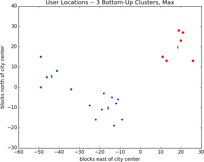
Figure 20-7. Three bottom-up clusters using max distance

For Further Exploration

• scikit-learn has an entire module, sklearn.cluster, that contains several clustering algorithms including KMeans and the Ward hierarchical clustering algorithm (which uses a different criterion for merging clusters than ours did).

• SciPy has two clustering models: scipy.cluster.vq, which does k-means, and scipy.cluster.hierarchy, which has a variety of hierarchical clustering algorithms.