
Chapter 5. Learning and Prediction
In this chapter, we’ll learn what our data means and how it drives our decision processes. Learning about our data gives us knowledge, and knowledge enables us to make reasonable guesses about what to expect in the future. This is the reason for the existence of data science: learning enough about the data so we can make predictions on newly arriving data. This can be as simple as categorizing data into groups or clusters. It can span a much broader set of processes that culminate (ultimately) in the path to artificial intelligence. Learning is divided into two major categories: unsupervised and supervised.
In general, we think of data as having variates X and responses Y, and our goal is to build a model using X so that we can predict what happens when we put in a new X. If we have the Y, we can “supervise” the building of the model. In many cases, we have only the variates X. The model will then have to be built in an unsupervised manner. Typical unsupervised methods include clustering, whereas supervised learning may include any of the regression methods (e.g., linear regression) or classification methods such as naive Bayes, logistic, or deep neural net classifiers. Many other methods and permutations of those methods exist, and covering them all would be impossible. Instead, here we dive into a few of the most useful ones.
Learning Algorithms
A few learning algorithms are prevalent in a large variety of techniques. In particular, we often use an iterative learning process to repeatedly optimize or update the model parameters we are searching for. Several methods are available for optimizing the parameters, and we cover the gradient descent method here.
Iterative Learning Procedure
One standard way to learn a model is to loop over a prediction state and update the state. Regression, clustering and expectation-maximization (EM) algorithms all benefit from similar forms of an iterative learning procedure. Our strategy here is to create a class that contains all the boilerplate iterative machinery, and then allow subclasses to define the explicit form of the prediction and parameter update methods.
publicclassIterativeLearningProcess{privatebooleanisConverged;privateintnumIterations;privateintmaxIterations;privatedoubleloss;privatedoubletolerance;privateintbatchSize;// if == 0 then uses ALL dataprivateLossFunctionlossFunction;publicIterativeLearningProcess(LossFunctionlossFunction){this.lossFunction=lossFunction;loss=0;isConverged=false;numIterations=0;maxIterations=200;tolerance=10E-6;batchSize=100;}publicvoidlearn(RealMatrixinput,RealMatrixtarget){doublepriorLoss=tolerance;numIterations=0;loss=0;isConverged=false;Batchbatch=newBatch(input,target);RealMatrixinputBatch;RealMatrixtargetBatch;while(numIterations<maxIterations&&!isConverged){if(batchSize>0&&batchSize<input.getRowDimension()){batch.calcNextBatch(batchSize);inputBatch=batch.getInputBatch();targetBatch=batch.getTargetBatch();}else{inputBatch=input;targetBatch=target;}RealMatrixoutputBatch=predict(inputBatch);loss=lossFunction.getMeanLoss(outputBatch,targetBatch);if(Math.abs(priorLoss-loss)<tolerance){isConverged=true;}else{update(inputBatch,targetBatch,outputBatch);priorLoss=loss;}numIterations++;}}publicRealMatrixpredict(RealMatrixinput){thrownewUnsupportedOperationException("Implement the predict method!");}publicvoidupdate(RealMatrixinput,RealMatrixtarget,RealMatrixoutput){thrownewUnsupportedOperationException("Implement the update method!");}}
Gradient Descent Optimizer
One way to learn parameters is via a gradient descent (an iterative first-order optimization algorithm). This optimizes the parameters by incrementally updating them with corrective learning (the error is used). The term stochastic means that we add one point at a time, as opposed to using the whole batch of data at once. In practice, it helps to use a mini-batch of about 100 points at a time, chosen at random in each step of the iterative learning process. The general idea is to minimize a loss function such that parameter updates are given by the following:

The parameter update is related to the gradient of an objective
function ![]() such that
such that

For deep networks, we will need to back-propagate this error through the network. We cover this in detail in “Deep Networks”.
For the purposes of this chapter, we can define an interface that returns a parameter update, given a particular gradient. Method signatures for both matrix and vector forms are included:
publicinterfaceOptimizer{RealMatrixgetWeightUpdate(RealMatrixweightGradient);RealVectorgetBiasUpdate(RealVectorbiasGradient);}
The most common case of gradient descent is to subtract the scaled gradient from the existing parameter such that

The update rule is as follows:

The most common type of stochastic gradient descent (SGD) is adding the update to the current parameters by using a learning rate:
publicclassGradientDescentimplementsOptimizer{privatedoublelearningRate;publicGradientDescent(doublelearningRate){this.learningRate=learningRate;}@OverridepublicRealMatrixgetWeightUpdate(RealMatrixweightGradient){returnweightGradient.scalarMultiply(-1.0*learningRate);}@OverridepublicRealVectorgetBiasUpdate(RealVectorbiasGradient){returnbiasGradient.mapMultiply(-1.0*learningRate);}}
One common extension to this optimizer is the inclusion of momentum, which slows the process as the optimum is reached, avoiding an overshoot of the correct parameters:

The update rule is as follows:

We see that adding momentum is easily accomplished by extending
the GradientDescent class, making provisions for storing
the most recent update to the weights and bias for calculation of the
next update. Note that the first time around, no prior updates will be
stored yet, so a new set is created (and initialized to zero):
publicclassGradientDescentMomentumextendsGradientDescent{privatefinaldoublemomentum;privateRealMatrixpriorWeightUpdate;privateRealVectorpriorBiasUpdate;publicGradientDescentMomentum(doublelearningRate,doublemomentum){super(learningRate);this.momentum=momentum;priorWeightUpdate=null;priorBiasUpdate=null;}@OverridepublicRealMatrixgetWeightUpdate(RealMatrixweightGradient){// creates matrix of zeros same size as gradients if// one does not already existif(priorWeightUpdate==null){priorWeightUpdate=newBlockRealMatrix(weightGradient.getRowDimension(),weightGradient.getColumnDimension());}RealMatrixupdate=priorWeightUpdate.scalarMultiply(momentum).subtract(super.getWeightUpdate(weightGradient));priorWeightUpdate=update;returnupdate;}@OverridepublicRealVectorgetBiasUpdate(RealVectorbiasGradient){if(priorBiasUpdate==null){priorBiasUpdate=newArrayRealVector(biasGradient.getDimension());}RealVectorupdate=priorBiasUpdate.mapMultiply(momentum).subtract(super.getBiasUpdate(biasGradient));priorBiasUpdate=update;returnupdate;}}
This is an ongoing and active field. By using this methodology, it is easy to extend capabilities by using ADAM or ADADELTA algorithms, for example.
Evaluating Learning Processes
Iterative processes can operate indefinitely. We always designate a maximum number of iterations we will allow so that any process cannot just run away and compute forever. Typically, this is on the order of 103 to 106 iterations, but there’s no rule. There is a way to stop the iterative process early if a certain criteria has been met. We call this convergence, and the idea is that our process has converged on an answer that appears to be a stable point in the computation (e.g., the free parameters are no longer changing in a large enough increment to warrant the continuation of the process). Of course, there is more than one way to do this. Although certain learning techniques lend themselves to specific convergence criteria, there is no universal method.
Minimizing a Loss Function
A loss function designates the loss between predicted and target outputs. It is also
known as a cost function or error
term. Given a singular input vector x, output vector y, and prediction vector ![]() , the loss of the sample is denoted with
, the loss of the sample is denoted with
![]() . The form of the loss function depends on the
underlying statistical distribution of the output data. In most cases,
the loss over p-dimensional output and prediction
is the sum of the scalar losses per dimension:
. The form of the loss function depends on the
underlying statistical distribution of the output data. In most cases,
the loss over p-dimensional output and prediction
is the sum of the scalar losses per dimension:

Because we often deal with batches of data, we then calculate the
mean loss ![]() over the whole batch. When we talk about minimizing
a loss function, we are minimizing the mean loss over the batch of data
that was input into the learning algorithm. In many cases, we can use
the gradient of the loss
over the whole batch. When we talk about minimizing
a loss function, we are minimizing the mean loss over the batch of data
that was input into the learning algorithm. In many cases, we can use
the gradient of the loss ![]() to apply corrective learning. Here the gradient of
the loss with respect to the predicted value
to apply corrective learning. Here the gradient of
the loss with respect to the predicted value ![]() can usually be computed with ease. The idea is then
to return a loss gradient that is the same shape as its input.
can usually be computed with ease. The idea is then
to return a loss gradient that is the same shape as its input.
Warning
In some texts, the output is denoted as ![]() (for truth or
target), and the prediction is denoted as
(for truth or
target), and the prediction is denoted as
![]() . In this text, we denote the output as
. In this text, we denote the output as
![]() and prediction as
and prediction as ![]() . Note that
. Note that ![]() has different meanings in these two cases.
has different meanings in these two cases.
Many forms are dependent on the type of variables (continuous or discrete or both) and the underlying statistical distribution. However, a common theme makes using an interface ideal. A reason for leaving implementation up to a specific class is that it takes advantage of optimized algorithms for linear algebra routines.
publicinterfaceLossFunction{publicdoublegetSampleLoss(doublepredicted,doubletarget);publicdoublegetSampleLoss(RealVectorpredicted,RealVectortarget);publicdoublegetMeanLoss(RealMatrixpredicted,RealMatrixtarget);publicdoublegetSampleLossGradient(doublepredicted,doubletarget);publicRealVectorgetSampleLossGradient(RealVectorpredicted,RealVectortarget);publicRealMatrixgetLossGradient(RealMatrixpredicted,RealMatrixtarget);}
Linear loss
Also known as the absolute loss, the linear loss is the absolute difference between the output and the prediction:

The gradient is misleading because of the absolute-value signs, which cannot be ignored:

The gradient is not defined at ![]() because
because ![]() has a discontinuity there. However, we can
programmatically designate the gradient function to set its value to 0
when the gradient is zero to avoid a 1/0 exception. In this way, the
gradient function returns only a –1, 0, or 1. Ideally, we then use the
mathematical function sign(x), which returns only
–1, 0, or 1, depending on the respective input values of x < 0, x =
0 and x > 0.
has a discontinuity there. However, we can
programmatically designate the gradient function to set its value to 0
when the gradient is zero to avoid a 1/0 exception. In this way, the
gradient function returns only a –1, 0, or 1. Ideally, we then use the
mathematical function sign(x), which returns only
–1, 0, or 1, depending on the respective input values of x < 0, x =
0 and x > 0.
publicclassLinearLossFunctionimplementsLossFunction{@OverridepublicdoublegetSampleLoss(doublepredicted,doubletarget){returnMath.abs(predicted-target);}@OverridepublicdoublegetSampleLoss(RealVectorpredicted,RealVectortarget){returnpredicted.getL1Distance(target);}@OverridepublicdoublegetMeanLoss(RealMatrixpredicted,RealMatrixtarget){SummaryStatisticsstats=newSummaryStatistics();for(inti=0;i<predicted.getRowDimension();i++){doubledist=getSampleLoss(predicted.getRowVector(i),target.getRowVector(i));stats.addValue(dist);}returnstats.getMean();}@OverridepublicdoublegetSampleLossGradient(doublepredicted,doubletarget){returnMath.signum(predicted-target);// -1, 0, 1}@OverridepublicRealVectorgetSampleLossGradient(RealVectorpredicted,RealVectortarget){returnpredicted.subtract(target).map(newSignum());}//YOUDO SparseToSignum would be nice!!! only process elements of the iterable@OverridepublicRealMatrixgetLossGradient(RealMatrixpredicted,RealMatrixtarget){RealMatrixloss=newArray2DRowRealMatrix(predicted.getRowDimension(),predicted.getColumnDimension());for(inti=0;i<predicted.getRowDimension();i++){loss.setRowVector(i,getSampleLossGradient(predicted.getRowVector(i),target.getRowVector(i)));}returnloss;}}
Quadratic loss
A generalized form for computing the error of a predictive process is by minimizing a distance metric such as L1 or L2 over the entire dataset. For a particular prediction-target pair, the quadratic error is as follows:

An element of the sample loss gradient is then as follows:

An implementation of a quadratic loss function follows:
publicclassQuadraticLossFunctionimplementsLossFunction{@OverridepublicdoublegetSampleLoss(doublepredicted,doubletarget){doublediff=predicted-target;return0.5*diff*diff;}@OverridepublicdoublegetSampleLoss(RealVectorpredicted,RealVectortarget){doubledist=predicted.getDistance(target);return0.5*dist*dist;}@OverridepublicdoublegetMeanLoss(RealMatrixpredicted,RealMatrixtarget){SummaryStatisticsstats=newSummaryStatistics();for(inti=0;i<predicted.getRowDimension();i++){doubledist=getSampleLoss(predicted.getRowVector(i),target.getRowVector(i));stats.addValue(dist);}returnstats.getMean();}@OverridepublicdoublegetSampleLossGradient(doublepredicted,doubletarget){returnpredicted-target;}@OverridepublicRealVectorgetSampleLossGradient(RealVectorpredicted,RealVectortarget){returnpredicted.subtract(target);}@OverridepublicRealMatrixgetLossGradient(RealMatrixpredicted,RealMatrixtarget){returnpredicted.subtract(target);}}
Cross-entropy loss
Cross entropy is great for classification (e.g., logistics regression or
neural nets). We discussed the origins of cross entropy in Chapter 3. Because cross entropy shows
similarity between two samples, it can be used for measuring agreement
between known and predicted values. In the case of learning
algorithms, we equate p with the known value
y, and q with the predicted
value ![]() . We set the loss equal to the cross entropy
. We set the loss equal to the cross entropy
![]() such that
such that ![]() where
where ![]() is the target (label) and
is the target (label) and ![]() is the i-th predicted value
for each class k in a K
multiclass output. The cross entropy (the loss per sample) is then as
follows:
is the i-th predicted value
for each class k in a K
multiclass output. The cross entropy (the loss per sample) is then as
follows:

There are several common forms for cross entropy and its associated loss function.
Bernoulli
In the case of Bernoulli output variates, the known outputs
y are binary, where the prediction probability
is ![]() , giving a cross-entropy loss:
, giving a cross-entropy loss:

The sample loss gradient is then as follows:

Here is an implementation of the Bernoulli cross-entropy loss:
publicclassCrossEntropyLossFunctionimplementsLossFunction{@OverridepublicdoublegetSampleLoss(doublepredicted,doubletarget){return-1.0*(target*((predicted>0)?FastMath.log(predicted):0)+(1.0-target)*(predicted<1?FastMath.log(1.0-predicted):0));}@OverridepublicdoublegetSampleLoss(RealVectorpredicted,RealVectortarget){doubleloss=0.0;for(inti=0;i<predicted.getDimension();i++){loss+=getSampleLoss(predicted.getEntry(i),target.getEntry(i));}returnloss;}@OverridepublicdoublegetMeanLoss(RealMatrixpredicted,RealMatrixtarget){SummaryStatisticsstats=newSummaryStatistics();for(inti=0;i<predicted.getRowDimension();i++){stats.addValue(getSampleLoss(predicted.getRowVector(i),target.getRowVector(i)));}returnstats.getMean();}@OverridepublicdoublegetSampleLossGradient(doublepredicted,doubletarget){// NOTE this blows up if predicted = 0 or 1, which it should never bereturn(predicted-target)/(predicted*(1-predicted));}@OverridepublicRealVectorgetSampleLossGradient(RealVectorpredicted,RealVectortarget){RealVectorloss=newArrayRealVector(predicted.getDimension());for(inti=0;i<predicted.getDimension();i++){loss.setEntry(i,getSampleLossGradient(predicted.getEntry(i),target.getEntry(i)));}returnloss;}@OverridepublicRealMatrixgetLossGradient(RealMatrixpredicted,RealMatrixtarget){RealMatrixloss=newArray2DRowRealMatrix(predicted.getRowDimension(),predicted.getColumnDimension());for(inti=0;i<predicted.getRowDimension();i++){loss.setRowVector(i,getSampleLossGradient(predicted.getRowVector(i),target.getRowVector(i)));}returnloss;}}
This expression is most often used with the logistic output function.
Multinomial
When the output is multiclass (k = 0,1,2 … K – 1) and transformed to a set of binary outputs via one-hot-encoding, the cross entropy loss is the sum over all possible classes:

However, in one-hot encoding, only one dimension has y = 1 and the rest are y = 0 (a sparse matrix). Therefore, the sample loss is also a sparse matrix. Ideally, we could simplify this calculation by taking that into account.
The sample loss gradient is as follows:

Because most of the loss matrix will be zeros, we need to calculate the gradient only for locations where y = 1. This form is used primarily with the softmax output function:
publicclassOneHotCrossEntropyLossFunctionimplementsLossFunction{@OverridepublicdoublegetSampleLoss(doublepredicted,doubletarget){returnpredicted>0?-1.0*target*FastMath.log(predicted):0;}@OverridepublicdoublegetSampleLoss(RealVectorpredicted,RealVectortarget){doublesampleLoss=0.0;for(inti=0;i<predicted.getDimension();i++){sampleLoss+=getSampleLoss(predicted.getEntry(i),target.getEntry(i));}returnsampleLoss;}@OverridepublicdoublegetMeanLoss(RealMatrixpredicted,RealMatrixtarget){SummaryStatisticsstats=newSummaryStatistics();for(inti=0;i<predicted.getRowDimension();i++){stats.addValue(getSampleLoss(predicted.getRowVector(i),target.getRowVector(i)));}returnstats.getMean();}@OverridepublicdoublegetSampleLossGradient(doublepredicted,doubletarget){return-1.0*target/predicted;}@OverridepublicRealVectorgetSampleLossGradient(RealVectorpredicted,RealVectortarget){returntarget.ebeDivide(predicted).mapMultiplyToSelf(-1.0);}@OverridepublicRealMatrixgetLossGradient(RealMatrixpredicted,RealMatrixtarget){RealMatrixloss=newArray2DRowRealMatrix(predicted.getRowDimension(),predicted.getColumnDimension());for(inti=0;i<predicted.getRowDimension();i++){loss.setRowVector(i,getSampleLossGradient(predicted.getRowVector(i),target.getRowVector(i)));}returnloss;}}
Two-Point
When the output is binary but takes on the values of –1 and 1
instead of 0 and 1, we can rescale for use with the Bernoulli
expression with the substitutions ![]() and
and ![]() :
:

The sample loss gradient is as follows:

The Java code is shown here:
publicclassTwoPointCrossEntropyLossFunctionimplementsLossFunction{@OverridepublicdoublegetSampleLoss(doublepredicted,doubletarget){// convert -1:1 to 0:1 scaledoubley=0.5*(predicted+1);doublet=0.5*(target+1);return-1.0*(t*((y>0)?FastMath.log(y):0)+(1.0-t)*(y<1?FastMath.log(1.0-y):0));}@OverridepublicdoublegetSampleLoss(RealVectorpredicted,RealVectortarget){doubleloss=0.0;for(inti=0;i<predicted.getDimension();i++){loss+=getSampleLoss(predicted.getEntry(i),target.getEntry(i));}returnloss;}@OverridepublicdoublegetMeanLoss(RealMatrixpredicted,RealMatrixtarget){SummaryStatisticsstats=newSummaryStatistics();for(inti=0;i<predicted.getRowDimension();i++){stats.addValue(getSampleLoss(predicted.getRowVector(i),target.getRowVector(i)));}returnstats.getMean();}@OverridepublicdoublegetSampleLossGradient(doublepredicted,doubletarget){return(predicted-target)/(1-predicted*predicted);}@OverridepublicRealVectorgetSampleLossGradient(RealVectorpredicted,RealVectortarget){RealVectorloss=newArrayRealVector(predicted.getDimension());for(inti=0;i<predicted.getDimension();i++){loss.setEntry(i,getSampleLossGradient(predicted.getEntry(i),target.getEntry(i)));}returnloss;}@OverridepublicRealMatrixgetLossGradient(RealMatrixpredicted,RealMatrixtarget){RealMatrixloss=newArray2DRowRealMatrix(predicted.getRowDimension(),predicted.getColumnDimension());for(inti=0;i<predicted.getRowDimension();i++){loss.setRowVector(i,getSampleLossGradient(predicted.getRowVector(i),target.getRowVector(i)));}returnloss;}}
This form of loss is compatible with a tanh activation function.
Minimizing the Sum of Variances
When data is split into more than one group, we can monitor the spread
of the group from its mean position via the variance. Because variances
add, we can define a metric s over
n groups, where ![]() is the variance of each group:
is the variance of each group:
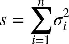
As s decreases, it signifies that the overall error of the procedure is also decreasing. This works great for clustering techniques, such as k-means, which are based on finding the mean value or center point of each cluster.
Silhouette Coefficient
In unsupervised learning techniques such as clustering, we seek to
discover how closely packed each group of points is. The
silhouette coefficient is a metric that relates the
difference between the minimum distance inside any given cluster and its
nearest cluster. The silhouette coefficient, s, is
the average over all distances ![]() for each sample; a = the mean
distance between that sample and all other points in the class, and
b = the mean
distance between that sample and all the points in the next nearest
cluster:
for each sample; a = the mean
distance between that sample and all other points in the class, and
b = the mean
distance between that sample and all the points in the next nearest
cluster:

Then the silhouette score is the mean of all the sample silhouette coefficients:

The silhouette score is between –1 and 1, where –1 is incorrect clustering, 1 is highly dense clustering, and 0 indicates overlapping clusters. s increases as clusters are dense and well separated. The goal is in monitor processes for a maximal value of s. Note that the silhouette coefficient is defined only for 2 <= nlabels <= nsamples – 1. Here is the Java code:
publicclassSilhouetteCoefficient{List<Cluster<DoublePoint>>clusters;doublecoefficient;intnumClusters;intnumSamples;publicSilhouetteCoefficient(List<Cluster<DoublePoint>>clusters){this.clusters=clusters;calculateMeanCoefficient();}privatevoidcalculateMeanCoefficient(){SummaryStatisticsstats=newSummaryStatistics();intclusterNumber=0;for(Cluster<DoublePoint>cluster:clusters){for(DoublePointpoint:cluster.getPoints()){doubles=calculateCoefficientForOnePoint(point,clusterNumber);stats.addValue(s);}clusterNumber++;}coefficient=stats.getMean();}privatedoublecalculateCoefficientForOnePoint(DoublePointonePoint,intclusterLabel){/* all other points will compared to this one */RealVectorvector=newArrayRealVector(onePoint.getPoint());doublea=0;doubleb=Double.MAX_VALUE;intclusterNumber=0;for(Cluster<DoublePoint>cluster:clusters){SummaryStatisticsclusterStats=newSummaryStatistics();for(DoublePointotherPoint:cluster.getPoints()){RealVectorotherVector=newArrayRealVector(otherPoint.getPoint());doubledist=vector.getDistance(otherVector);clusterStats.addValue(dist);}doubleavgDistance=clusterStats.getMean();if(clusterNumber==clusterLabel){/* we have included a 0 distance of point with itself *//* and need to subtract it out of the mean */doublen=newLong(clusterStats.getN()).doubleValue();doublecorrection=n/(n-1.0);a=correction*avgDistance;}else{b=Math.min(avgDistance,b);}clusterNumber++;}return(b-a)/Math.max(a,b);}}
Log-Likelihood
In unsupervised learning problems for which each outcome prediction has a
probability associated with it, we can utilize the log-likelihood. One
particular example is the Gaussian clustering example in this chapter.
For this expectation-maximization algorithm, a mixture of multivariate
normal distributions are optimized to fit the data. Each data point has
a probability density ![]() associated with it, given the overlying model, and
the log-likelihood can be computed as the mean of the log of the
probabilities for each point:
associated with it, given the overlying model, and
the log-likelihood can be computed as the mean of the log of the
probabilities for each point:

We can then accumulate the average log-likelihood over all the
data points ![]() . In the case of the Gaussian clustering example,
we can obtain this parameter directly via the
. In the case of the Gaussian clustering example,
we can obtain this parameter directly via the
MultivariateNormalMixtureExpectationMaximization.getLogLikelihood()
method.
Classifier Accuracy
How do we know how accurate a classifier really is? A binary classification scheme has four possible outcomes:
true positive (TP)—both data and prediction have the value of 1
true negative (TN)—both data and prediction have a value of 0
Given a tally of each of the four possible outcomes, we can calculate, among other things, the accuracy of the classifier.
Accuracy is calculated as follows:

Or, considering that the denominator is the total number of rows in the dataset N, the expression is equivalent to the following:

We can then calculate the accuracy for each dimension. The average of the accuracy vector is the average accuracy of the classifier. This is also the Jaccard score.
In the special case that we are using one-hot-encoding we require only true positives and the accuracy per dimension is then as folllows:

Nt is the total class count (of 1s) for that dimension. The accuracy score for the classifier is then as follows:

In this implementation, we have two use cases. In one case, there is one-hot encoding. In the other case, the binary, multilabel outputs are independent. In that case, we can choose a threshold (between 0 and 1) at which point to decide whether the class is 1 or 0. In the most basic sense, we can choose the threshold to be 0.5, where all probabilities below 0.5 are classified as 0, and probabilities greater than or equal to 0.5 are classified as 1. Examples of this class’s use are in “Supervised Learning”.
publicclassClassifierAccuracy{RealMatrixpredictions;RealMatrixtargets;ProbabilityEncoderprobabilityEncoder;RealVectorclassCount;publicClassifierAccuracy(RealMatrixpredictions,RealMatrixtargets){this.predictions=predictions;this.targets=targets;probabilityEncoder=newProbabilityEncoder();//tally the binary class occurrences per dimensionclassCount=newArrayRealVector(targets.getColumnDimension());for(inti=0;i<targets.getRowDimension();i++){classCount=classCount.add(targets.getRowVector(i));}}publicRealVectorgetAccuracyPerDimension(){RealVectoraccuracy=newArrayRealVector(predictions.getColumnDimension());for(inti=0;i<predictions.getRowDimension();i++){RealVectorbinarized=probabilityEncoder.getOneHot(predictions.getRowVector(i));// 0*0, 0*1, 1*0 = 0 and ONLY 1*1 = 1 gives true positivesRealVectordecision=binarized.ebeMultiply(targets.getRowVector(i));// append TP counts to accuracyaccuracy=accuracy.add(decision);}returnaccuracy.ebeDivide(classCount);}publicdoublegetAccuracy(){// convert accuracy_per_dim back to counts// then sum and divide by total rowsreturngetAccuracyPerDimension().ebeMultiply(classCount).getL1Norm()/targets.getRowDimension();}// implements Jaccard similarity scorespublicRealVectorgetAccuracyPerDimension(doublethreshold){// assumes un-correlated multi-outputRealVectoraccuracy=newArrayRealVector(targets.getColumnDimension());for(inti=0;i<predictions.getRowDimension();i++){//binarize the row vector according to the thresholdRealVectorbinarized=probabilityEncoder.getBinary(predictions.getRowVector(i),threshold);// 0-0 (TN) and 1-1 (TP) = 0 while 1-0 = 1 and 0-1 = -1RealVectordecision=binarized.subtract(targets.getRowVector(i)).map(newAbs()).mapMultiply(-1).mapAdd(1);// append either TP and TN counts to accuracyaccuracy=accuracy.add(decision);}returnaccuracy.mapDivide((double)predictions.getRowDimension());// accuracy for each dimension, given the threshold}publicdoublegetAccuracy(doublethreshold){// mean of the accuracy vectorreturngetAccuracyPerDimension(threshold).getL1Norm()/targets.getColumnDimension();}}
Unsupervised Learning
When we have only independent variables, we must discern patterns in the data without the
aid of dependent variables (responses) or labels. The most common of the
unsupervised techniques is clustering. The goal of all clustering is to
classify each data point X into a series
of K sets, ![]() , where the number of sets is less than the number of
points. Typically, each point
, where the number of sets is less than the number of
points. Typically, each point ![]() will belong to only one subset
will belong to only one subset ![]() . However, we can also designate each point
. However, we can also designate each point
![]() to belong to all sets with a probability
to belong to all sets with a probability
![]() such that the sum = 1. Here we explore two varieties
of hard assignment,
k-means and DBSCAN clustering; and a soft assignment type, mixture of
Gaussians. They all vary widely in their assumptions, algorithms, and
scope. However, the result is generally the same: to classify a point
X into one or more subsets, or
clusters.
such that the sum = 1. Here we explore two varieties
of hard assignment,
k-means and DBSCAN clustering; and a soft assignment type, mixture of
Gaussians. They all vary widely in their assumptions, algorithms, and
scope. However, the result is generally the same: to classify a point
X into one or more subsets, or
clusters.
k-Means Clustering
k-means is the simplest form of clustering and uses hard assignment to
find the cluster centers for a predetermined number of clusters.
Initially, an integer number of K clusters is
chosen to start with, and the centroid location ![]() of each is chosen by an algorithm (or at random). A
point x will belong to a cluster of set
of each is chosen by an algorithm (or at random). A
point x will belong to a cluster of set
![]() if its Euclidean distance (can be others, but
usually L2) is closest to
if its Euclidean distance (can be others, but
usually L2) is closest to ![]() . Then the objective function to minimize is as
follows:
. Then the objective function to minimize is as
follows:

Then we update the new centroid (the mean position of all x in a cluster) via this equation:

We can stop when L does not change anymore, and therefore the centroids are not changing. How do we know what number of clusters is optimal? We can keep track of the sum of all cluster variances and vary the number of clusters. When plotting the sum-of-variances versus the number of clusters, ideally the shape will look like a hockey stick, with a sharp bend in the plot indicating the ideal number of clusters at the point.

The algorithm used by Apache Commons Math is the k-means++,
which does a better job of picking out random starting points. The
class KMeansPlusPlusClusterer<T> takes
several arguments in its constructor, but only one is required: the
number of clusters to search for. The data to be clustered must be a
List of Clusterable points. The class
DoublePoint is a convenient wrapper around an array of doubles that
implements Clusterable. It takes an array of
doubles in its constructor.
double[][]rawData=...List<DoublePoint>data=newArrayList<>();for(double[]row:rawData){data.add(newDoublePoint(row));}/* num clusters to search for */intnumClusters=1;/* the basic constructor */KMeansPlusPlusClusterer<DoublePoint>kmpp=newKMeansPlusPlusClusterer<>(numClusters);/* this performs the clustering and returns a list with length numClusters */List<CentroidCluster<DoublePoint>>results=kmpp.cluster(data);/* iterate the list of Clusterables */for(CentroidCluster<DoublePoint>result:results){DoublePointcentroid=(DoublePoint)result.getCenter();System.out.println(centroid);// DoublePoint has toString() method/* we also have access to all the points in only this cluster */List<DoublePoint>clusterPoints=result.getPoints();}
In the k-means scheme, we want to iterate
over several choices of numClusters, keeping track of the
sum of variances for each cluster. Because variances add, this gives us
a measure of total error. Ideally, we want to minimize this number. Here
we keep track of the cluster variances as we iterate through various
cluster searches:
/* search for 1 through 5 clusters */for(inti=1;i<5;i++){KMeansPlusPlusClusterer<DoublePoint>kmpp=newKMeansPlusPlusClusterer<>(i);List<CentroidCluster<DoublePoint>>results=kmpp.cluster(data);/* this is the sum of variances for this number of clusters */SumOfClusterVariances<DoublePoint>clusterVar=newSumOfClusterVariances<>(newEuclideanDistance());for(CentroidCluster<DoublePoint>result:results){DoublePointcentroid=(DoublePoint)result.getCenter());}}
One way we can improve the k-means is to try
several starting points and take the best result—that is, lowest error.
Because the starting points are random, at times the clustering
algorithm takes a wrong turn, which even our strategies for handling
empty clusters can’t handle. It’s a good idea to repeat each clustering
attempt and choose the one with the best results. The class
MultiKMeansPlusPlusClusterer<T> performs the same clustering operation numTrials
times and uses only the best result. We can combine these with the
previous code:
/* repeat each clustering trial 10 times and take the best */intnumTrials=10;/* search for 1 through 5 clusters */for(inti=1;i<5;i++){/* we still need to create a cluster instance ... */KMeansPlusPlusClusterer<DoublePoint>kmpp=newKMeansPlusPlusClusterer<>(i);/* ... and pass it to the constructor of the multi */MultiKMeansPlusPlusClusterer<DoublePoint>multiKMPP=newMultiKMeansPlusPlusClusterer<>(kmpp,numTrials);/* NOTE this clusters on multiKMPP NOT kmpp */List<CentroidCluster<DoublePoint>>results=multikKMPP.cluster(data);/* this is the sum of variances for this number of clusters */SumOfClusterVariances<DoublePoint>clusterVar=newSumOfClusterVariances<>(newEuclideanDistance());/* the sumOfVariance score for 'i' clusters */doublescore=clusterVar.score(results)/* the 'best' centroids */for(CentroidCluster<DoublePoint>result:results){DoublePointcentroid=(DoublePoint)result.getCenter());}}
DBSCAN
What if clusters have irregular shapes? What if clusters are intertwined? The DBSCAN (density-based spatial clustering of applications with noise) algorithm is ideal for finding hard-to-classify clusters. It does not assume the number of clusters, but rather optimizes itself to the number of clusters present. The only input parameters are the maximum radius of capture and the minimum number of points per cluster. It is implemented as follows:
/* constructor takes eps and minpoints */doubleeps=2.0;intminPts=3;DBSCANClustererclusterer=newDBSCANClusterer(eps,minPts);List<Cluster<DoublePoint>>results=clusterer.cluster(data);
Note that unlike the previous k-means++,
DBSCAN does not return a CentroidCluster type because the
centroids of the irregularly shaped clusters may not be meaningful.
Instead, you can access the clustered points directly and use them for
further processing. But also note that if the algorithm cannot find any
clusters, the List<Cluster<T>> instance will
comprise an empty List with a size of 0:
if(results.isEmpty()){System.out.println("No clusters were found");}else{for(Cluster<DoublePoint>result:results){/* each clusters points are in here */List<DoublePoint>points=result.getPoints();System.out.println(points.size());// TODO do something with the points in each cluster}}
In this example, we have created four random multivariate (two-dimensional) normal clusters. Of note is that two of the clusters are close enough to be touching and could even be considered one angular-shaped cluster. This demonstrates a trade-off in the DBSCAN algorithm.
In this case, we need to set the radius of capture small enough
(![]() = 0.225) to allow detection of the separate
clusters, but there are outliers. A larger radius (
= 0.225) to allow detection of the separate
clusters, but there are outliers. A larger radius (![]() = 0.8) here would combine the two leftmost clusters
into one, but there would be almost no outliers. As we decrease
= 0.8) here would combine the two leftmost clusters
into one, but there would be almost no outliers. As we decrease
![]() , we are enabling a finer resolution for cluster
detection, but we also are increasing the likelihood of outliers. This
may become less of an issue in higher-dimensional space in which
clusters in close proximity to each other are less likely. An example of
four Gaussian clusters that fit the DBSCAN algorithm is shown in Figure 5-1.
, we are enabling a finer resolution for cluster
detection, but we also are increasing the likelihood of outliers. This
may become less of an issue in higher-dimensional space in which
clusters in close proximity to each other are less likely. An example of
four Gaussian clusters that fit the DBSCAN algorithm is shown in Figure 5-1.

Figure 5-1. DBSCAN on simulation of four Gaussian clusters
Dealing with outliers
The DBSCAN algorithm is well suited for dealing with outliers. How do we access them? Unfortunately, the current Math implementation does not allow access to the points labeled as noise in the DBSCAN algorithm. But we can try to keep track of that like this:
/* we are going to keep track of outliers */// NOTE need a completely new list, not to reference same object// e.g., outliers = data is not a good idea// List<DoublePoint> outliers = data; // will remove points from data as wellList<DoublePoint>outliers=newArrayList<>();for(DoublePointdp:data){outliers.add(newDoublePoint(dp.getPoint()));}
Then when we are iterating through the results clusters, we can remove each cluster from the complete dataset data, which will become the outliers after we remove everything else:
for(Cluster<DoublePoint>result:results){/* each clusters points are in here */List<DoublePoint>points=result.getPoints();/* remove these cluster points from the data copy "outliers"which will contain ONLY the outliers after all of thecluster points are removed*/outliers.removeAll(points);}// now the LIST outliers only contains points NOT in any cluster
Optimizing radius of capture and minPoints
The radius of capture is easy to see in 2D, but how do you know what is optimal? Clearly, this is entirely subjective and will depend on your use case. In general, the number of minimum points should follow this relation:

So in a 2D case, we at least want three minimum points per
cluster. The radius of capture, ![]() , can be estimated at the bend in hockey stick of
the k-distance graph. Both the number of minimum
points and the radius of capture can be grid-searched against the
silhouette score as a metric. First, find the silhouette coefficient,
s, for each sample; a = the
mean distance between that sample and all other points in the class,
and b = the mean distance between that sample and
all the points in the next nearest cluster:
, can be estimated at the bend in hockey stick of
the k-distance graph. Both the number of minimum
points and the radius of capture can be grid-searched against the
silhouette score as a metric. First, find the silhouette coefficient,
s, for each sample; a = the
mean distance between that sample and all other points in the class,
and b = the mean distance between that sample and
all the points in the next nearest cluster:

Then the silhouette score is the mean of all the sample
silhouette coefficients. The silhouette score is between –1 and 1: –1
is incorrect clustering, 1 is highly dense clustering, and 0 indicates
overlapping clusters. s increases as clusters are
dense and well separated. As in the case for
k-means previously, we can vary the
![]() value and output the silhouette score:
value and output the silhouette score:
double[]epsVals={0.15,0.16,0.17,0.18,0.19,0.20,0.21,0.22,0.23,0.24,0.25};for(doubleepsVal:epsVals){DBSCANClustererclusterer=newDBSCANClusterer(epsVal,minPts);List<Cluster<DoublePoint>>results=clusterer.cluster(dbExam.clusterPoints);if(results.isEmpty()){System.out.println("No clusters where found");}else{SilhouetteCoefficients=newSilhouetteCoefficient(results);System.out.println("eps = "+epsVal+" numClusters = "+results.size()+" s = "+s.getCoefficient());}}
This gives the following output:
eps = 0.15 numClusters = 7 s = 0.54765
eps = 0.16 numClusters = 7 s = 0.53424
eps = 0.17 numClusters = 7 s = 0.53311
eps = 0.18 numClusters = 6 s = 0.68734
eps = 0.19 numClusters = 6 s = 0.68342
eps = 0.20 numClusters = 6 s = 0.67743
eps = 0.21 numClusters = 5 s = 0.68348
eps = 0.22 numClusters = 4 s = 0.70073 // best one!
eps = 0.23 numClusters = 3 s = 0.68861
eps = 0.24 numClusters = 3 s = 0.68766
eps = 0.25 numClusters = 3 s = 0.68571
We see a bump in the silhouette score at ![]() = 0.22, where s = 0.7,
indicating that the ideal
= 0.22, where s = 0.7,
indicating that the ideal ![]() is approximately 0.22. At this particular
is approximately 0.22. At this particular
![]() , the DBSCAN routine also converged on four
clusters, which is the number we simulated. In practical situations,
of course, we won’t know the number of clusters beforehand. But this
example does indicate that s should approach a
maximal value of 1 if we have the right number of clusters and
therefore the right
, the DBSCAN routine also converged on four
clusters, which is the number we simulated. In practical situations,
of course, we won’t know the number of clusters beforehand. But this
example does indicate that s should approach a
maximal value of 1 if we have the right number of clusters and
therefore the right ![]() .
.
Inference from DBSCAN
DBSCAN is not for predicting membership of new points as in the k-means algorithm. It is for segmenting the data for further use. If you want a predictive model based on DBSCAN, you can assign class values to the clustered data points and try a classification scheme such as Gaussian, naive Bayes, or others.
Gaussian Mixtures
A similar concept to DBSCAN is to cluster based on the density of points, but use the multivariate normal distribution N(μ, Σ) because it comprises a mean and covariance. Data points located near the mean have the highest probability of belonging to that cluster, whereas the probability drops off to almost nothing as the data point is located very far from the mean.
Gaussian mixture model
A Gaussian mixture model is expressed mathematically as a weighted mixture of k multivariate Gaussian distributions (as discussed in Chapter 3).

Here the weights satisfy the relation ![]() . We must create a
. We must create a List of
Pair objects, where the first member of Pair
is the weight, and the second member is the distribution
itself:
List<Pair<Double,MultivariateNormalDistribution>>mixture=newArrayList<>();/* mixture component 1 */doublealphaOne=0.70;double[]meansOne={0.0,0.0};double[][]covOne={{1.0,0.0},{0.0,1.0}};MultivariateNormalDistributiondistOne=newMultivariateNormalDistribution(meansOne,covOne);PairpairOne=newPair(alphaOne,distOne);mixture.add(pairOne);/* mixture component 2 */doublealphaTwo=0.30;double[]meansTwo={5.0,5.0};double[][]covTwo={{1.0,0.0},{0.0,1.0}};MultivariateNormalDistributiondistTwo=newMultivariateNormalDistribution(meansTwo,covTwo);PairpairTwo=newPair(alphaTwo,distTwo);mixture.add(pairTwo);/* add the list of pairs to the mixture model and sample the points */MixtureMultivariateNormalDistributiondist=newMixtureMultivariateNormalDistribution(mixture);/* we don't need a seed, but it helps if we want to recall the same data */dist.reseedRandomGenerator(0L);/* generate 1000 random data points from the mixture */double[][]data=dist.sample(1000);
Note that the data sampled from the distribution mixture model
does not keep track of what component the sampled data point comes
from. In other words, you will not be able to tell what
MultivariateNormal each sampled data point belongs to. If you require this
feature, you can always sample from the individual distributions and
then add them together later.
For purposes of testing, creating mixture models can be tedious and is fraught with problems. If you are not building a dataset from existing, real data, it is best to try simulating data with some known problems averted. A method for generating random mixture-model, is presented in Appendix A. In Figure 5-2, a plot of a multivariate Gaussian mixture model is demonstrated. There are two clusters in two dimensions.

Figure 5-2. Gaussian clusters in 2D
The data can be generated with the example code:
intdimension=5;intnumClusters=7;doubleboxSize=10;longseed=0L;intnumPoints=10000;/* see Appendix for this dataset */MultiNormalMixtureDatasetmnd=newMultiNormalMixtureDataset(dimension);mnd.createRandomMixtureModel(numClusters,boxSize,0L);double[][]data=mnd.getSimulatedData(numPoints);
Fitting with the EM algorithm
The expectation maximization algorithm is useful in many other places. Essentially, what is the
maximum likelihood that the parameters we’ve chosen are correct? We
iterate until they don’t change anymore, given a certain tolerance. We
need to provide a starting guess of what the mixture is. Using the
method in the preceding section, we can create a mixture with known
components. However, the static method
MultivariateNormalMixtureExpectationMaximization.estimate(data,
        numClusters)
is used to estimate the starting point given the
dataset and number of clusters as input:
MultivariateNormalMixtureExpectationMaximizationmixEM=newMultivariateNormalMixtureExpectationMaximization(data);/* need a guess as where to start */MixtureMultivariateNormalDistributioninitialMixture=MultivariateNormalMixtureExpectationMaximization.estimate(data,numClusters);/* perform the fit */mixEM.fit(initialMixture);/* this is the fitted model */MixtureMultivariateNormalDistributionfittedModel=mixEM.getFittedModel();for(Pair<Double,MultivariateNormalDistribution>pair:fittedModel.getComponents()){System.out.println("************ cluster *****************");System.out.println("alpha: "+pair.getFirst());System.out.println("means: "+newArrayRealVector(pair.getSecond().getMeans()));System.out.println("covar: "+pair.getSecond().getCovariances());}
Optimizing the number of clusters
Just as in k-means clustering, we would like to know the optimal number of clusters needed to describe our data. In this case, though, each data point belongs to all clusters with finite probability (soft assignment). How do we know when the number of clusters is good enough? We start with a low number (e.g., 2) and work our way up, calculating the log-likelihood for each trial. To make things easier, we can plot the loss (the negative of the log-likelihood), and watch as it hopefully drops toward zero. Realistically, it never will, but the idea is to stop when the loss becomes somewhat constant. Usually, the best number of clusters will be at the elbow of the hockey stick.
Here is the code:
MultivariateNormalMixtureExpectationMaximizationmixEM=newMultivariateNormalMixtureExpectationMaximization(data);intminNumClusters=2;intmaxNumClusters=10;for(inti=minNumCluster;i<=maxNumClusters;i++){/* need a guess as where to start */MixtureMultivariateNormalDistributioninitialMixture=MultivariateNormalMixtureExpectationMaximization.estimate(data,i);/* perform the fit */mixEM.fit(initialMixture);/* this is the fitted model */MixtureMultivariateNormalDistributionfittedModel=mixEM.getFittedModel();/* print out the log-likelihood */System.out.println(i+" ll: "+mixEM.getLogLikelihood());}
This outputs the following:
2ll:-6.3706437873501353ll:-5.9078649287863434ll:-5.57892467492610145ll:-5.3660409274931856ll:-5.0933916832173867ll:-5.19349105582161658ll:-4.9848375075478369ll:-4.981776514549066410ll:-4.981307556011888
When plotted, this shows a characteristic hockey-stick shape
with the inflection point at numClusters = 7, the number
of clusters we simulated. Note that we could have stored the
loglikelihoods in an array, and fit the results in a List
for later retrieval programatically. In Figure 5-3,
the log-likelihood loss is plotted versus the number of clusters. Note
the sharp decline in loss and the bend around seven clusters, the
original number of clusters in the simulated dataset.

Figure 5-3. Log loss of 7, 5 dimensional clusters
Supervised Learning
Given numeric variates X and potentially non-numeric responses Y, how can we formulate mathematical models to learn and predict? Recall that linear regression models rely on both X and Y to be continuous variables (e.g., real numbers). Even when Y contains 0s or 1s, (and any other integers), a linear regression would most likely fail.
Here we examine methods specifically designed for the common use cases that collect numeric data as variates and their associated labels. Most classification schemes lend themselves easily to a multidimensional variate X and a single dimension of classes Y. However, several techniques, including neural networks, can handle multiple output classes Y in a way analogous to the multiresponse models of linear regression.
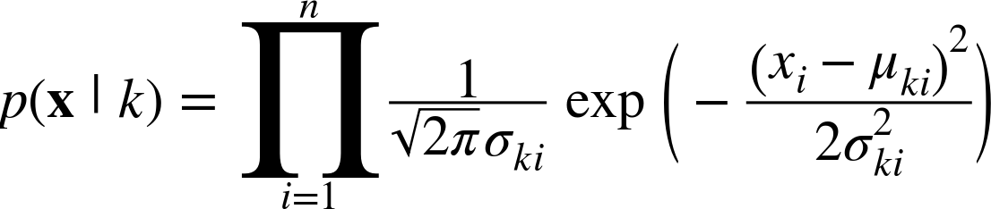
Naive Bayes
Naive Bayes is perhaps the most elementary of classification schemes and is a logical next step after clustering. Recall that in clustering, our goal is to separate or classify data into distinct groups. We can then look at each group individually and try to learn something about that group, such as its center position, its variance, or any other statistical measure.
In a naive Bayes classification scheme, we split the data into groups (classes) for each label type. We then learn something about the variates in each group. This will depend on the type of variable. For example, if the variables are real numbers, we can assume that each dimension (variate) of the data is a sample from a normal distribution.
For integer data (counts), we can assume a multinomial distribution. If the data is binary (0 or 1), we can assume a Bernoulli distributed dataset. In this way, we can estimate statistical quantities such as mean and variance for each of the datasets belonging to only the class it was labeled for. Note that unlike more sophisticated classification schemes, we never use the labels themselves in any computation or error propagation. They serve the purpose only of splitting our data into groups.
According to Bayes’ theorem (posterior = prior × likelihood /
evidence), the joint probability is the prior × likelihood. In our case,
the evidence is the sum of joint probabilities over all classes. For a
set of K classes, where k =
{1, 2 … K}, the probability of a particular class
![]() given an input vector x is determined as follows:
given an input vector x is determined as follows:

Here, the naive independence assumption allows us to express the likelihood as the product of probabilities for each dimension of the n-dimensional variate x:

This is expressed more compactly as follows:

The normalization is the sum over all terms in the numerator expressed:

The probability of any class is the number of times it occurs
divided by the total: ![]() . Here we take the product for each class
k over each feature
. Here we take the product for each class
k over each feature ![]() . The form of
. The form of ![]() , is probability density function we choose based on
our assumptions of the data. In the following sections, we explore
normal, multinomial, and Bernoulli distributions.
, is probability density function we choose based on
our assumptions of the data. In the following sections, we explore
normal, multinomial, and Bernoulli distributions.
Warning
Note that if any one calculation ![]() , the entire expression will be
, the entire expression will be ![]() . For some conditional probability models such as
Gaussian or Bernoulli distributions, this will never be the case. But
for a multinomial distribution, this can occur, so we include a small
factor
. For some conditional probability models such as
Gaussian or Bernoulli distributions, this will never be the case. But
for a multinomial distribution, this can occur, so we include a small
factor ![]() to avoid this.
to avoid this.
After we calculate posterior probabilities for each class, a Bayes classifier is then a decision rule on the posterior probabilities, where we take the maximum position as the most likely class:

We can use the same class for all types, because training the
model relies on the types of quantities that are easily accumulated
with MultivariateSummaryStatistics per class.
We can then use a strategy pattern to implement whichever type of
conditional probability we require and pass it directly into the
constructor:
publicclassNaiveBayes{Map<Integer,MultivariateSummaryStatistics>statistics;ConditionalProbabilityEstimatorconditionalProbabilityEstimator;intnumberOfPoints;// total number of points the model was trained onpublicNaiveBayes(ConditionalProbabilityEstimatorconditionalProbabilityEstimator){statistics=newHashMap<>();this.conditionalProbabilityEstimator=conditionalProbabilityEstimator;numberOfPoints=0;}publicvoidlearn(RealMatrixinput,RealMatrixtarget){// if numTargetCols == 1 then multiclass e.g. 0, 1, 2, 3// else one-hot e.g. 1000, 0100, 0010, 0001numberOfPoints+=input.getRowDimension();for(inti=0;i<input.getRowDimension();i++){double[]rowData=input.getRow(i);intlabel;if(target.getColumnDimension()==1){label=newDouble(target.getEntry(i,0)).intValue();}else{label=target.getRowVector(i).getMaxIndex();}if(!statistics.containsKey(label)){statistics.put(label,newMultivariateSummaryStatistics(rowData.length,true));}statistics.get(label).addValue(rowData);}}publicRealMatrixpredict(RealMatrixinput){intnumRows=input.getRowDimension();intnumCols=statistics.size();RealMatrixpredictions=newArray2DRowRealMatrix(numRows,numCols);for(inti=0;i<numRows;i++){double[]rowData=input.getRow(i);double[]probs=newdouble[numCols];doublesumProbs=0;for(Map.Entry<Integer,MultivariateSummaryStatistics>entrySet:statistics.entrySet()){IntegerclassNumber=entrySet.getKey();MultivariateSummaryStatisticsmss=entrySet.getValue();/* prior prob n_k / N ie num points in class / total points */doubleprob=newLong(mss.getN()).doubleValue()/numberOfPoints;/* depends on type ... Gaussian, Multinomial, or Bernoulli */prob*=conditionalProbabilityEstimator.getProbability(mss,rowData);probs[classNumber]=prob;sumProbs+=prob;}/* L1 norm the probs */for(intj=0;j<numCols;j++){probs[j]/=sumProbs;}predictions.setRow(i,probs);}returnpredictions;}}
All that is needed then is an interface that designates the form of the conditional probability:
publicinterfaceConditionalProbabilityEstimator{publicdoublegetProbability(MultivariateSummaryStatisticsmss,double[]features);}
In the following three subsections, we explore three kinds of
naive Bayes classifiers, each of which implements the
ConditionalProbabilityEstimator interface for use in
the NaiveBayes class.
Gaussian
If the features are continuous variables, we can use the Gaussian naive Bayes classifier:
We can then implement a class like this:
importorg.apache.commons.math3.distribution.NormalDistribution;importorg.apache.commons.math3.stat.descriptive.MultivariateSummaryStatistics;publicclassGaussianConditionalProbabilityEstimatorimplementsConditionalProbabilityEstimator{@OverridepublicdoublegetProbability(MultivariateSummaryStatisticsmss,double[]features){double[]means=mss.getMean();double[]stds=mss.getStandardDeviation();doubleprob=1.0;for(inti=0;i<features.length;i++){prob*=newNormalDistribution(means[i],stds[i]).density(features[i]);}returnprob;}}
And test it like this:
double[][]features={{6,180,12},{5.92,190,11},{5.58,170,12},{5.92,165,10},{5,100,6},{5.5,150,8},{5.42,130,7},{5.75,150,9}};String[]labels={"male","male","male","male","female","female","female","female"};NaiveBayesnb=newNaiveBayes(newGaussianConditionalProbabilityEstimator());nb.train(features,labels);double[]test={6,130,8};Stringinference=nb.inference(test);// "female"
This will yield the correct result, female.
Multinomial
Features are integer values—for example, counts. However, continuous
features such as TFIDF also can work. The likelihood of observing any
feature vector x for class ![]() is as follows:
is as follows:

We note that the front part of the term depends only on the input vector x, and therefore is equivalent for each calculation of p(x|k). Fortunately, this computationally intense term will drop out in the final, normalized expression for p(k|x), allowing us to use the much simpler formulation:

We can easily calculate the required probability ![]() where
where ![]() is the sum of values for each feature, given class
k, and
is the sum of values for each feature, given class
k, and ![]() is the total count for all features, given class
k. When estimating the conditional probabilities,
any zeros will cancel out the entire calculation. It is therefore
useful to estimate the probabilities with a small additive factor
is the total count for all features, given class
k. When estimating the conditional probabilities,
any zeros will cancel out the entire calculation. It is therefore
useful to estimate the probabilities with a small additive factor
![]() —known as Lidstone smoothing
for generalized
—known as Lidstone smoothing
for generalized ![]() , and Laplace smoothing when
, and Laplace smoothing when
![]() . As a result of this L1 normalization of the
numerator, the factor
. As a result of this L1 normalization of the
numerator, the factor ![]() is just the dimension of the feature
vector.
is just the dimension of the feature
vector.

The final expression is as follows:

For large ![]() (large counts of words, for example), the problem
may become numerically intractable. We can solve the problem in log
space and convert it back by using the relation
(large counts of words, for example), the problem
may become numerically intractable. We can solve the problem in log
space and convert it back by using the relation ![]() . The preceding expression can be written as
follows:
. The preceding expression can be written as
follows:

In this strategy implementation, the smoothing coefficient is
designated in the constructor. Note the use of the logarithmic
implementation to avoid numerical instability. It would be wise to add
an assertion (in the constructor) that the smoothing constant alpha
hold the relation ![]() :
:
publicclassMultinomialConditionalProbabilityEstimatorimplementsConditionalProbabilityEstimator{privatedoublealpha;publicMultinomialConditionalProbabilityEstimator(doublealpha){this.alpha=alpha;// Lidstone smoothing 0 > alpha > 1}publicMultinomialConditionalProbabilityEstimator(){this(1);// Laplace smoothing}@OverridepublicdoublegetProbability(MultivariateSummaryStatisticsmss,double[]features){intn=features.length;doubleprob=0;double[]sum=mss.getSum();// array of x_i sums for this classdoubletotal=0.0;// total count of all featuresfor(inti=0;i<n;i++){total+=sum[i];}for(inti=0;i<n;i++){prob+=features[i]*Math.log((sum[i]+alpha)/(total+alpha*n));}returnMath.exp(prob);}}
Bernoulli
Features are binary values—for example, occupancy status. The probability per feature is the mean value for that column. For an input feature, we can then calculate the probability:

In other words, if the input feature is a 1, the probability for that feature is the mean value for the column. If the input feature is a 0, the probability for that feature is 1 – mean of that column. We implement the Bernoulli conditional probability as shown here:
publicclassBernoulliConditionalProbabilityEstimatorimplementsConditionalProbabilityEstimator{@OverridepublicdoublegetProbability(MultivariateSummaryStatisticsmss,double[]features){intn=features.length;double[]means=mss.getMean();// this is actually the prob per features e.g. count / totaldoubleprob=1.0;for(inti=0;i<n;i++){// if x_i = 1, then p, if x_i = 0 then 1-p, but here x_i is a doubleprob*=(features[i]>0.0)?means[i]:1-means[i];}returnprob;}}
Iris example
Try the Iris dataset by using a Gaussian conditional probability estimator:
Irisiris=newIris();MatrixResamplermr=newMatrixResampler(iris.getFeatures(),iris.getLabels());mr.calculateTestTrainSplit(0.4,0L);NaiveBayesnb=newNaiveBayes(newGaussianConditionalProbabilityEstimator());nb.learn(mr.getTrainingFeatures(),mr.getTrainingLabels());RealMatrixpredictions=nb.predict(mr.getTestingFeatures());ClassifierAccuracyacc=newClassifierAccuracy(predictions,mr.getTestingLabels());System.out.println(acc.getAccuracyPerDimension());// {1; 1; 0.9642857143}System.out.println(acc.getAccuracy());// 0.9833333333333333
Linear Models
If we rotate, translate, and scale a dataset X,
can we relate it to the output Y by
mapping a function? In general, these all seek to solve the problem in
which an input matrix X is the data,
and W and b are the free parameters we want to optimize
for. Using the notation developed in Chapter 2, for a weighted input matrix and
intercept Z = XW + hbT, we apply a function ![]() (Z) to each element of Z to compute a prediction matrix
(Z) to each element of Z to compute a prediction matrix ![]() such that
such that
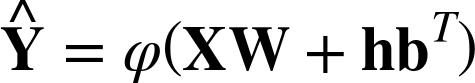
We can view a linear model as a box with input X and predicted output ![]() . When optimizing the free parameters W and b, the
error on the output can be sent back through the box, providing
incremental updates dependent on the algorithm chosen. Of note is that
we can even pass the error back to the input, calculating the error on
the input. For linear models, this is not necessary, but as we will see
in “Deep Networks”, this is essential for the
back-propagation algorithm. A generalized linear model is shown in Figure 5-4.
. When optimizing the free parameters W and b, the
error on the output can be sent back through the box, providing
incremental updates dependent on the algorithm chosen. Of note is that
we can even pass the error back to the input, calculating the error on
the input. For linear models, this is not necessary, but as we will see
in “Deep Networks”, this is essential for the
back-propagation algorithm. A generalized linear model is shown in Figure 5-4.

Figure 5-4. Linear model
We can then implement a LinearModel class that is
responsible only for holding the type of output function, the state of
the free parameters, and simple methods for updating the
parameters:
publicclassLinearModel{privateRealMatrixweight;privateRealVectorbias;privatefinalOutputFunctionoutputFunction;publicLinearModel(intinputDimension,intoutputDimension,OutputFunctionoutputFunction){weight=MatrixOperations.getUniformRandomMatrix(inputDimension,outputDimension,0L);bias=MatrixOperations.getUniformRandomVector(outputDimension,0L);this.outputFunction=outputFunction;}publicRealMatrixgetOutput(RealMatrixinput){returnoutputFunction.getOutput(input,weight,bias);}publicvoidaddUpdateToWeight(RealMatrixweightUpdate){weight=weight.add(weightUpdate);}publicvoidaddUpdateToBias(RealVectorbiasUpdate){bias=bias.add(biasUpdate);}}
The interface for an output function is shown here:
publicinterfaceOutputFunction{RealMatrixgetOutput(RealMatrixinput,RealMatrixweight,RealVectorbias);RealMatrixgetDelta(RealMatrixerror,RealMatrixoutput);}
In most cases, we can never precisely determine W and b such that the relation between X and Y is exact. The best we can do is to estimate
Y, calling it ![]() , and then proceed to minimize a loss function of our
choice
, and then proceed to minimize a loss function of our
choice ![]() . The goal is then to incrementally update the values
of W and b over a set of iterations (annotated by
t) according to the following:
. The goal is then to incrementally update the values
of W and b over a set of iterations (annotated by
t) according to the following:


In this section, we will focus on the use of the gradient descent algorithm for determining the values of W and b. Recalling that the loss function is ultimately a function of both W and b, we can use the gradient descent optimizer to make the incremental updates with the gradient of the loss:


The objective function to be optimized is the mean loss
![]() , where the gradient of any particular term with
respect to a parameter
, where the gradient of any particular term with
respect to a parameter ![]() and
and ![]() can be expressed as follows:
can be expressed as follows:

The first term is the derivative of the loss function, which we covered in the prior section. The second part of the term is the derivative of the output function:

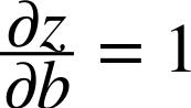
The third term is simply the derivative of z with respect to either w or b:

As we will see, the choice of the appropriate pair of loss function and output function will lead to a mathematical simplification that leads to the delta rule. In this case, the updates to the weights and bias are always as follows:


When the mean loss ![]() stops changing within a certain numerical tolerance
(e.g., 10E – 6), the process can stop, and we assume W and b are at their optimal values. However, iterative
algorithms are prone to iterate forever because of numerical oddities.
Therefore, all iterative solvers will set a maximum number of iterations
(e.g., 1,000), after which the process will terminate. It is good
practice to always check whether the maximum number of iterations was
reached, because the change in loss may still be high, indicating that
the optimal values of the free parameters have not yet been attained.
The form of both the transformation function
stops changing within a certain numerical tolerance
(e.g., 10E – 6), the process can stop, and we assume W and b are at their optimal values. However, iterative
algorithms are prone to iterate forever because of numerical oddities.
Therefore, all iterative solvers will set a maximum number of iterations
(e.g., 1,000), after which the process will terminate. It is good
practice to always check whether the maximum number of iterations was
reached, because the change in loss may still be high, indicating that
the optimal values of the free parameters have not yet been attained.
The form of both the transformation function ![]() (Z) and the loss function
(Z) and the loss function ![]() will depend on the problem at hand. Several common
scenarios are detailed next.
will depend on the problem at hand. Several common
scenarios are detailed next.
Linear
In the case of linear regression, ![]() (Z) is set to the identity function, and the output is
equivalent to the input:
(Z) is set to the identity function, and the output is
equivalent to the input:

This provides the familiar form of a linear regression model:

We solved this problem in both Chapters 2 and 3 by using different methods. In the case of Chapter 2, we solved for the free parameters by posing the problem in matrix notation and then using a back-solver, whereas in Chapter 3 we took the least-squares approach. There are, however, even more ways to solve this problem! Ridge regression, lasso regression, and elastic nets are just a few examples. The idea is to eliminate variables that are not useful by penalizing their parameters during the optimization process:
publicclassLinearOutputFunctionimplementsOutputFunction{@OverridepublicRealMatrixgetOutput(RealMatrixinput,RealMatrixweight,RealVectorbias){returnMatrixOperations.XWplusB(input,weight,bias);}@OverridepublicRealMatrixgetDelta(RealMatrixerrorGradient,RealMatrixoutput){// output gradient is all 1's ... so just return errorGradientreturnerrorGradient;}}
Logistic
Solve the problem where y is a 0 or 1 that can also
be multidimensional, such as y = 0,1,1,0,1. The nonlinear function ![]()
For gradient descent, we need the derivative of the function:

It is convenient to note that the derivative may also be
expressed in terms of the original function. This is useful, because
it allows us to reuse the calculated values of ![]() rather than having to recompute all the
computationally costly matrix algebra:
rather than having to recompute all the
computationally costly matrix algebra:

In the case of gradient descent, we can then implement it as follows:
publicclassLogisticOutputFunctionimplementsOutputFunction{@OverridepublicRealMatrixgetOutput(RealMatrixinput,RealMatrixweight,RealVectorbias){returnMatrixOperations.XWplusB(input,weight,bias,newSigmoid());}@OverridepublicRealMatrixgetDelta(RealMatrixerrorGradient,RealMatrixoutput){// this changes output permanentlyoutput.walkInOptimizedOrder(newUnivariateFunctionMapper(newLogisticGradient()));// output is now the output gradientreturnMatrixOperations.ebeMultiply(errorGradient,output);}privateclassLogisticGradientimplementsUnivariateFunction{@Overridepublicdoublevalue(doublex){returnx*(1-x);}}}
When using the cross-entropy loss function to calculate the loss
term, note that ![]() such that:
such that:

So it then reduces to this:

And considering

the gradient of the loss with respect to the weight is as follows:

We can include a learning rate η to slow the update process. The final formulas, adapted for use with matrices of data, are given as follows:


Here, h is an
m-dimensional vector of 1s. Notice the inclusion
of the learning rate ![]() , which usually takes on values between 0.0001 and
1 and limits how fast the parameters converge. For small values of
, which usually takes on values between 0.0001 and
1 and limits how fast the parameters converge. For small values of
![]() , we are more likely to find the correct values of
the weights, but at the cost of performing many more time-consuming
iterations. For larger values of
, we are more likely to find the correct values of
the weights, but at the cost of performing many more time-consuming
iterations. For larger values of ![]() , we will complete the algorithmic learning task
much quicker. However, we may inadvertently skip over the best
solution, giving nonsensical values for the weights.
, we will complete the algorithmic learning task
much quicker. However, we may inadvertently skip over the best
solution, giving nonsensical values for the weights.
Softmax
Softmax is similar to logistic regression, but the target variable can be
multinomial (an integer between 0 and numClasses – 1). We
then transform the output with one-hot encoding such that Y = {0,0,1,0}. Note that unlike multi-output
logistic regression, only one position in each row can be set to 1,
and all others must be 0. Each element of the transformed matrix is
then exponentiated and then L1 normalized row-wise:

Because the derivative involves more than one variable, the Jacobian takes the place of the gradient with terms:
Then for a single p-dimensional output and prediction, we can calculate the quantity:

This simplifies to the following:

Each term has the exact same update rule as the other linear models under gradient descent:

As a practical matter, it will take two passes over the input to compute the softmax output. First, we raise each argument by the exponential function, keeping track of the running sum. Then we iterate over that list again, dividing each term by the running sum. If (and only if) we use the softmax cross entropy as an error, the update formula for the coefficients is identical to that of logistic regression. We show this calculation explicitly in “Deep Networks”.
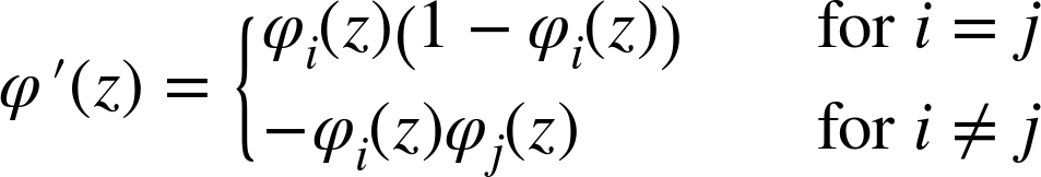
publicclassSoftmaxOutputFunctionimplementsOutputFunction{@OverridepublicRealMatrixgetOutput(RealMatrixinput,RealMatrixweight,RealVectorbias){RealMatrixoutput=MatrixOperations.XWplusB(input,weight,bias,newExp());MatrixScaler.l1(output);returnoutput;}@OverridepublicRealMatrixgetDelta(RealMatrixerror,RealMatrixoutput){RealMatrixdelta=newBlockRealMatrix(error.getRowDimension(),error.getColumnDimension());for(inti=0;i<output.getRowDimension();i++){delta.setRowVector(i,getJacobian(output.getRowVector(i)).preMultiply(error.getRowVector(i)));}returndelta;}privateRealMatrixgetJacobian(RealVectoroutput){intnumRows=output.getDimension();intnumCols=output.getDimension();RealMatrixjacobian=newBlockRealMatrix(numRows,numCols);for(inti=0;i<numRows;i++){doubleoutput_i=output.getEntry(i);for(intj=i;j<numCols;j++){doubleoutput_j=output.getEntry(j);if(i==j){jacobian.setEntry(i,i,output_i*(1-output_i));}else{jacobian.setEntry(i,j,-1.0*output_i*output_j);jacobian.setEntry(j,i,-1.0*output_j*output_i);}}}returnjacobian;}}
Tanh
Another common activation function utilizes the hyperbolic tangent
![]() with the form shown here:
with the form shown here:


Once again, the derivative ![]() reuses the value calculated from
reuses the value calculated from ![]() :
:
publicclassTanhOutputFunctionimplementsOutputFunction{@OverridepublicRealMatrixgetOutput(RealMatrixinput,RealMatrixweight,RealVectorbias){returnMatrixOperations.XWplusB(input,weight,bias,newTanh());}@OverridepublicRealMatrixgetDelta(RealMatrixerrorGradient,RealMatrixoutput){// this changes output permanentlyoutput.walkInOptimizedOrder(newUnivariateFunctionMapper(newTanhGradient()));// output is now the output gradientreturnMatrixOperations.ebeMultiply(errorGradient,output);}privateclassTanhGradientimplementsUnivariateFunction{@Overridepublicdoublevalue(doublex){return(1-x*x);}}}
Linear model estimator
Using the gradient descent algorithm and the appropriate loss functions, we can build a simple linear estimator that updates the parameters iteratively using the delta rule. This applies only if the correct pairing of output function and loss function are used, as shown in Table 5-1.
| Output function | Loss function |
|---|---|
| Linear | Quadratic |
| Logistic | Bernoulli cross-entropy |
| Softmax | Multinomial cross-entropy |
| Tanh | Two-point cross-entropy |
We can then extend the IterativeLearningProcess
class and add code for the output function prediction and
updates:
publicclassLinearModelEstimatorextendsIterativeLearningProcess{privatefinalLinearModellinearModel;privatefinalOptimizeroptimizer;publicLinearModelEstimator(LinearModellinearModel,LossFunctionlossFunction,Optimizeroptimizer){super(lossFunction);this.linearModel=linearModel;this.optimizer=optimizer;}@OverridepublicRealMatrixpredict(RealMatrixinput){returnlinearModel.getOutput(input);}@Overrideprotectedvoidupdate(RealMatrixinput,RealMatrixtarget,RealMatrixoutput){RealMatrixweightGradient=input.transpose().multiply(output.subtract(target));RealMatrixweightUpdate=optimizer.getWeightUpdate(weightGradient);linearModel.addUpdateToWeight(weightUpdate);RealVectorh=newArrayRealVector(input.getRowDimension(),1.0);RealVectorbiasGradient=output.subtract(target).preMultiply(h);RealVectorbiasUpdate=optimizer.getBiasUpdate(biasGradient);linearModel.addUpdateToBias(biasUpdate);}publicLinearModelgetLinearModel(){returnlinearModel;}publicOptimizergetOptimizer(){returnoptimizer;}}
Iris example
The Iris dataset is a great example to explore a linear classifier:
/* get data and split into train / test sets */Irisiris=newIris();MatrixResamplerresampler=newMatrixResampler(iris.getFeatures(),iris.getLabels());resampler.calculateTestTrainSplit(0.40,0L);/* set up the linear estimator */LinearModelEstimatorestimator=newLinearModelEstimator(newLinearModel(4,3,newSoftmaxOutputFunction()),newSoftMaxCrossEntropyLossFunction(),newDeltaRule(0.001));estimator.setBatchSize(0);estimator.setMaxIterations(6000);estimator.setTolerance(10E-6);/* learn the model parameters */estimator.learn(resampler.getTrainingFeatures(),resampler.getTrainingLabels());/* predict on test data */RealMatrixprediction=estimator.predict(resampler.getTestingFeatures());/* results */ClassifierAccuracyaccuracy=newClassifierAccuracy(prediction,resampler.getTestingLabels());estimator.isConverged();// trueestimator.getNumIterations();// 3094estimator.getLoss();// 0.0769accuracy.getAccuracy();// 0.983accuracy.getAccuracyPerDimension();// {1.0, 0.92, 1.0}
Deep Networks
Feeding the output of a linear model into another linear model creates a nonlinear system capable of modeling complicated behavior. A system with multiple layers is known as a deep network. While a linear model has an input and output, a deep network adds multiple “hidden” layers between the input and output. Most explanations of deep networks address the input, hidden, and output layers as separate quantities. In this book, however, we take the alternative viewpoint that a deep network is nothing more than a composition of linear models. We can then view a deep network purely as a linear algebra problem. Figure 5-5 demonstrates how a multilayer neural network can be viewed as a chain of linear models.

Figure 5-5. Deep network
A network layer
We can extend the concept of a linear model to the form of a
network layer where we must persist the input, output, and errors. The
code for the network layer is then an extension of the
LinearModel class:
publicclassNetworkLayerextendsLinearModel{RealMatrixinput;RealMatrixinputError;RealMatrixoutput;RealMatrixoutputError;Optimizeroptimizer;publicNetworkLayer(intinputDimension,intoutputDimension,OutputFunctionoutputFunction,Optimizeroptimizer){super(inputDimension,outputDimension,outputFunction);this.optimizer=optimizer;}publicvoidupdate(){//back propagate error/* D = eps o f'(XW) where o is Hadamard productor J f'(XW) where J is Jacobian */RealMatrixdeltas=getOutputFunction().getDelta(outputError,output);/* E_out = D W^T */inputError=deltas.multiply(getWeight().transpose());/* W = W - alpha * delta * input */RealMatrixweightGradient=input.transpose().multiply(deltas);/* w_{t+1} = w_{t} + delta w_{t} */addUpdateToWeight(optimizer.getWeightUpdate(weightGradient));// this essentially sums the columns of delta and that vector is grad_bRealVectorh=newArrayRealVector(input.getRowDimension(),1.0);RealVectorbiasGradient=deltas.preMultiply(h);addUpdateToBias(optimizer.getBiasUpdate(biasGradient));}}
Feed forward
To calculate the network output, we must feed the input through each layer of the network in the forward direction. The network input X1 is used to compute the output of the first layer:

We set the first-layer output to the second-layer input:

The output of the second layer is shown here:

In general, the output of each layer l after the first layer is expressed in terms of the prior-layer output:

The feed-forward process for L layers then appears as a series of nested linear models:

Another simpler way to write this expression is as a composition of functions:

In addition to unique weights, each layer can take a different form for the activation function. In this way, it is clear that a feed-forward, deep neural network (a.k.a. multilayer perceptron) is nothing more than a composition of arbitrary linear models. The result, however, is a rather complex nonlinear model.
Back propagation
At this point, we need to back-propagate the network output error. For
the last layer (the output layer), we back-propagate the loss gradient
![]() . For compatible loss function–output function
pairs, this is identical to a linear model estimator. As formulated in
“Gradient Descent Optimizer”, it is then convenient to define a new
quantity, the layer delta, D, which
is the matrix multiplication of Yerr with the tensor of
output function Jacobians:
. For compatible loss function–output function
pairs, this is identical to a linear model estimator. As formulated in
“Gradient Descent Optimizer”, it is then convenient to define a new
quantity, the layer delta, D, which
is the matrix multiplication of Yerr with the tensor of
output function Jacobians:

In most cases, the gradient of the output function will suffice and the prior expression can be simplified as as follows:

We store the quantity D since it is used in two places that must be calculated in order. The back-propagated error is updated first:

The weight and bias gradients are then calculated as follows,
where h is an ![]() -length vector of 1s.
-length vector of 1s.
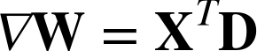

Note that the expression hTD is the equivalent of summing each column of D. The layer weights can then be updated using the optimization rule of choice (usually gradient descent of some variety). That completes all the calculations needed for the network layer! Then set the Yerr of the next layer down to the freshly calculated Xerr and repeat the process until the first layer’s parameters are updated.
Warning
Make sure to calculate the back-propagated error before updating the weight!
Deep network estimator
Learning the parameters of a deep network is accomplished with the
same iterative process as a linear model. In this case, the entire feed-forward process acts as one prediction step and the back propagation
process acts as one update step. We implement a deep network estimator by extending the
IterativeLearningProcess and building layers of linear
models subclassed as NetworkLayers:
publicclassDeepNetworkextendsIterativeLearningProcess{privatefinalList<NetworkLayer>layers;publicDeepNetwork(){this.layers=newArrayList<>();}publicvoidaddLayer(NetworkLayernetworkLayer){layers.add(networkLayer);}@OverridepublicRealMatrixpredict(RealMatrixinput){/* the initial input MUST BE DEEP COPIED or is overwritten */RealMatrixlayerInput=input.copy();for(NetworkLayerlayer:layers){layer.setInput(layerInput);/* calc the output and set to next layer input*/RealMatrixoutput=layer.getOutput(layerInput);layer.setOutput(output);/*does not need a deep copy, but be aware thatevery layer input shares memory of prior layer output*/layerInput=output;}/* layerInput is holding the final output ... get a deep copy */returnlayerInput.copy();}@Overrideprotectedvoidupdate(RealMatrixinput,RealMatrixtarget,RealMatrixoutput){/* gradient of the network error and starts the back prop process */RealMatrixlayerError=getLossFunction().getLossGradient(output,target).copy();/* create list iterator and set cursor to last! */ListIteratorli=layers.listIterator(layers.size());while(li.hasPrevious()){NetworkLayerlayer=(NetworkLayer)li.previous();/* get error input from higher layer */layer.setOutputError(layerError);/* this back propagates the error and updates weights */layer.update();/* pass along error to next layer down */layerError=layer.getInputError();}}}
MNIST example
MNIST, the classic handwritten digits dataset, is often used for testing learning algorithms. Here we get 94 percent accuracy by using a simple network with two hidden layers:
MNISTmnist=newMNIST();DeepNetworknetwork=newDeepNetwork();/* input, hidden and output layers */network.addLayer(newNetworkLayer(784,500,newTanhOutputFunction(),newGradientDescentMomentum(0.0001,0.95)));network.addLayer(newNetworkLayer(500,300,newTanhOutputFunction(),newGradientDescentMomentum(0.0001,0.95)));network.addLayer(newNetworkLayer(300,10,newSoftmaxOutputFunction(),newGradientDescentMomentum(0.0001,0.95)));/* runtime parameters */network.setLossFunction(newSoftMaxCrossEntropyLossFunction());network.setMaxIterations(6000);network.setTolerance(10E-9);network.setBatchSize(100);/* learn */network.learn(mnist.trainingData,mnist.trainingLabels);/* predict */RealMatrixprediction=network.predict(mnist.testingData);/* compute accuracy */ClassifierAccuracyaccuracy=newClassifierAccuracy(prediction,mnist.testingLabels);/* results */network.isConverged();// falsenetwork.getNumIterations();// 10000network.getLoss();// 0.00633accuracy.getAccuracy();// 0.94