
Chapter 2. Linear Algebra
Now that we have spent a whole chapter acquiring data in some format or another, we will most likely end up viewing the data (in our minds) in the form of spreadsheet. It is natural to envision the names of each column going across from left to right (age, address, ID number, etc.), with each row representing a unique record or data point. Much of data science comes down to this exact formulation. What we are seeking to find is a relationship between any number of columns of interest (which we will call variables) and any number of columns that indicate a measurable outcome (which we will call responses).
Typically, we use the letter ![]() to denote the variables, and
to denote the variables, and ![]() for the responses. Likewise, the responses can be
designated by a matrix Y that has a number of columns
for the responses. Likewise, the responses can be
designated by a matrix Y that has a number of columns ![]() and must have the same number of rows
and must have the same number of rows ![]() as X does. Note that in many cases, there is only one
dimension of response variable such that
as X does. Note that in many cases, there is only one
dimension of response variable such that ![]() . However, it helps to generalize linear algebra problems
to arbitrary dimensions.
. However, it helps to generalize linear algebra problems
to arbitrary dimensions.
In general, the main idea behind linear algebra is to find a relationship between X and Y. The simplest of these is to ask whether we can multiply X by a new matrix of yet-to-be-determined values W, such that the result is exactly (or nearly) equal to Y. An example of XW = Y looks like this:
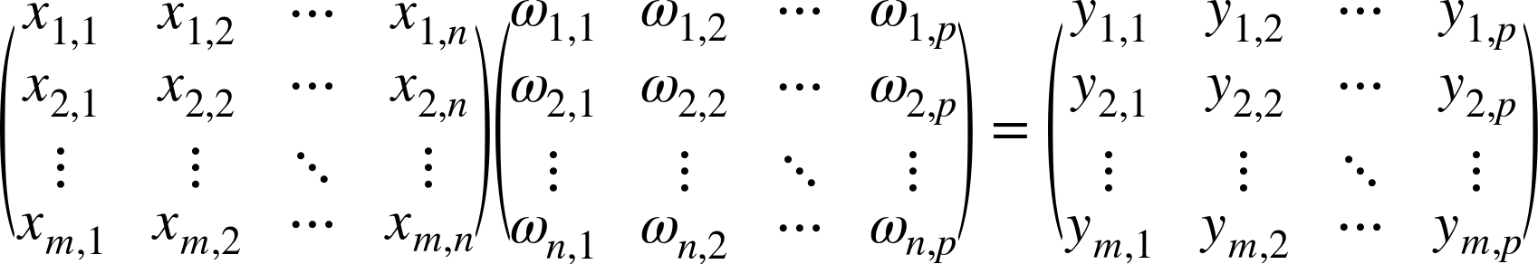
Keep in mind that as the equation is drawn, the sizes of the matrices
look similar. This can be misleading, because in most cases the number of
data points ![]() is large, perhaps
in the millions or billions, while the number of columns
is large, perhaps
in the millions or billions, while the number of columns ![]() for the respective X and Y matrices is usually much smaller (from tens to
hundreds). You will then take notice that regardless of the size of
for the respective X and Y matrices is usually much smaller (from tens to
hundreds). You will then take notice that regardless of the size of
![]() (e.g., 100,000), the size of the W matrix is independent of
(e.g., 100,000), the size of the W matrix is independent of ![]() ; its size is
; its size is ![]() (e.g., 10 × 10). And this is the heart of linear
algebra: that we can explain the contents of extremely large data structures
such as X and Y by using a much more compact data structure
W. The rules of linear algebra enable us to express any
particular value of Y in terms of a row of X and column of W. For example the value of
(e.g., 10 × 10). And this is the heart of linear
algebra: that we can explain the contents of extremely large data structures
such as X and Y by using a much more compact data structure
W. The rules of linear algebra enable us to express any
particular value of Y in terms of a row of X and column of W. For example the value of ![]() is written out as follows:
is written out as follows:

In the rest of this chapter, we will work out the rules and operations of linear algebra, and in the final section show the solution to the linear system XW = Y. More advanced topics in data science such as those presented in Chapters 4 and 5, will rely heavily on the use of linear algebra.
Building Vectors and Matrices
Despite any formal definitions, a vector is just a
one-dimensional array of a defined length. Many examples may come to mind.
You might have an array of integers representing the counts per day of a
web metric. Maybe you have a large number of “features” in an array that
will be used for input into a machine-learning routine. Or perhaps you are
keeping track of geometric coordinates such as x and
y, and you might create an array for each pair
[x,y]. While we can argue the philosophical meaning of what a
vector is (i.e., an element of vector space with magnitude and direction),
as long as you are consistent in how you define your vectors throughout
the problem you are solving, then all the mathematical formulations will
work beautifully, without any concern for the topic of study.
In general, a vector x has the following form, comprising n components:

Likewise, a matrix A is just a two-dimensional array with m rows and n columns:

A vector can also be represented in matrix notation as a column vector:

Warning
We use bold lowercase letters to represent vectors and use bold uppercase letters to represent matrices. Note that the vector x can also be represented as a column of the matrix X.
In practice, vectors and matrices are useful to data scientists. A common example is a dataset in which (feature) vectors are stacked on top of each other, and usually the number of rows m is much larger than the number of columns n. In essence, this type of data structure is really a list of vectors, but putting them in matrix form enables efficient calculation of all sorts of linear algebra quantities. Another type of matrix encountered in data science is one in which the components represent a relationship between the variables, such as a covariance or correlation matrix.
Array Storage
The Apache Commons Math library offers several options for creating
vectors and matrices of real numbers with the respective
RealVector and RealMatrix classes. Three of the most useful constructor types allocate an
empty instance of known dimension, create an instance from an array of
values, and create an instance by deep copying an existing instance,
respectively. To instantiate an empty,
n-dimensional vector of type
RealVector, use the ArrayRealVector class
with an integer size:
intsize=3;RealVectorvector=newArrayRealVector(size);
If you already have an array of values, a vector can be created with that array as a constructor argument:
double[]data={1.0,2.2,4.5};RealVectorvector=newArrayRealVector(data);
A new vector can also be created by deep copying an existing vector into a new instance:
RealVectorvector=newArrayRealVector(realVector);
To set a default value for all elements of a vector, include that value in the constructor along with the size:
intsize=3;doubledefaultValue=1.0;RealVectorvector=newArrayRealVector(size,defaultValue);
A similar set of constructors follows for instantiating matrices, an empty matrix of known dimensions is instantiated with the following:
introwDimension=10;intcolDimension=20;RealMatrixmatrix=newArray2DRowRealMatrix(rowDimension,colDimension);
Or if you already have a two-dimensional array of doubles, you can pass it to the constructor:
double[][]data={{1.0,2.2,3.3},{2.2,6.2,6.3},{3.3,6.3,5.1}};RealMatrixmatrix=newArray2DRowRealMatrix(data);
Although there is no method for setting the entire matrix to a default value (as there is with a vector), instantiating a new matrix sets all elements to zero, so we can easily add a value to each element afterward:
introwDimension=10;intcolDimension=20;doubledefaultValue=1.0;RealMatrixmatrix=newArray2DRowRealMatrix(rowDimension,colDimension);matrix.scalarAdd(defaultValue);
Making a deep copy of a matrix may be performed via the RealMatrix.copy() method:
/* deep copy contents of matrix */RealMatrixanotherMatrix=matrix.copy();
Block Storage
For large matrices with dimensions greater than 50, it is recommended to use block
storage with the BlockRealMatrix class. Block storage
is an alternative to the two-dimensional array storage discussed in the
previous section. In this case, a large matrix is subdivided into
smaller blocks of data that are easier to cache and therefore easier to
operate on. To allocate space for a matrix, use the following
constructor:
RealMatrixblockMatrix=newBlockRealMatrix(50,50);
Or if you already have the data in a 2D array, use this constructor:
double[][]data=;RealMatrixblockMatrix=newBlockRealMatrix(data);
Map Storage
When a large vector or matrix is almost entirely zeros, it is termed
sparse. Because it is not efficient to store all
those zeros, only the positions and values of the nonzero elements are
stored. Behind the scenes, this is easily achieved by storing the
values in a HashMap. To create a sparse vector of known dimension, use the
following:
intdim=10000;RealVectorsparseVector=newOpenMapRealVector(dim);
And to create a sparse matrix, just add another dimension:
introws=10000;intcols=10000;RealMatrixsparseMatrix=newOpenMapRealMatrix(rows,cols);
Accessing Elements
Regardless of the type of storage backing the vector or matrix, the methods for assigning values and later retrieving them are equivalent.
Caution
Although the linear algebra theory presented in this book uses an index starting at 1, Java uses a 0-based index system. Keep this in mind as you translate algorithms from theory to code and in particular, when setting and getting values.
Setting and getting values uses the setEntry(int index, double value)
and getEntry(int
index) methods:
/* set the first value of v */vector.setEntry(0,1.2)/* and get it */doubleval=vector.getEntry(0);
To set all the values for a vector, use the set(double value) method:
/* zero the vector */vector.set(0);
However, if v is a sparse vector,
there is no point to setting all the values. In sparse algebra, missing
values are assumed to be zero. Instead, just use setEntry
to set only the values that are nonzero. To retrieve all the values of
an existing vector as an array of doubles, use the toArray() method:
double[]vals=vector.toArray();
Similar setting and getting is provided for matrices, regardless
of storage. Use the setEntry(int row, int column, double
value) and getEntry(int row, int column)
methods:
/* set first row, 3 column to 3.14 */matrix.setEntry(0,2,3.14);/* and get it */doubleval=matrix.getEntry(0,2);
Unlike the vector classes, there is no set() method
to set all the values of a matrix to one value. As long as the matrix
has all entries set to 0, as is the case for a newly constructed matrix,
you can set all the entries to one value by adding a constant with code
like this:
/* for an existing new matrix */matrix.scalarAdd(defaultValue);
Just as with sparse vectors, setting all the values to 0 for each i,j pair of a sparse matrix is not useful.
To get all the values of a matrix in the form of an array of
doubles, use the getData() method:
double[][]matrixData=matrix.getData();
Working with Submatrices
We often need to work with only a specific part of a matrix or want to
include a smaller matrix in a larger one. The RealMatrix
class contains several useful methods for dealing with these common
cases. For an existing matrix, there are two ways to create a submatrix
from it. The first method selects a rectangular region from the source
matrix and uses those entries to create a new matrix. The selected
rectangular region is defined by the point of origin, the upper-left
corner of the source matrix, and the lower-right corner defining the
area that should be included. It is invoked as RealMatrix.getSubMatrix(int startRow, int endRow,
int startColumn, int endColumn) and returns a
RealMatrix object with dimensions and values determined by
the selection. Note that the endRow and
endColumn values are inclusive.
double[][]data={{1,2,3},{4,5,6},{7,8,9}};RealMatrixm=newArray2DRowRealMatrix(data);intstartRow=0;intendRow=1;intstartColumn=1;intendColumn=2;RealMatrixsubM=m.getSubMatrix(startRow,endRow,startColumn,endColumn);// {{2,3},{5,6}}
We can also get specific rows and specific columns of a matrix.
This is achieved by creating an array of integers designating the row
and column indices we wish to keep. The method then takes both of these
arrays as RealMatrix.getSubMatrix(int[] selectedRows, int[]
selectedColumns). The three use cases are then as follows:
/* get selected rows and all columns */int[]selectedRows={0,2};int[]selectedCols={0,1,2};RealMatrixsubM=m.getSubMatrix(selectedRows,selectedColumns);// {{1,2,3},{7,8,9}}/* get all rows and selected columns */int[]selectedRows={0,1,2};int[]selectedCols={0,2};RealMatrixsubM=m.getSubMatrix(selectedRows,selectedColumns);// {{1,3},{4,6},{7,9}}/* get selected rows and selected columns */int[]selectedRows={0,2};int[]selectedCols={1};RealMatrixsubM=m.getSubMatrix(selectedRows,selectedColumns);// {{2},{8}}
We can also create a matrix in parts by setting the values of a
submatrix. We do this by adding a double array of data to an existing
matrix at the coordinates specified by row and column in RealMatrix.setSubMatrix(double[][] subMatrix, int
row, int column):
double[][]newData={{-3,-2},{-1,0}};introw=0;intcolumn=0;m.setSubMatrix(newData,row,column);// {{-3,-2,3},{-1,0,6},{7,8,9}}
Randomization
In learning algorithms, we often want to set all the values of a matrix (or
vectors) to random numbers. We can choose the statistical distribution
that implements the AbstractRealDistribution interface or
just go with the easy constructor, which picks random numbers between –1
and 1. We can pass in an existing matrix or vector to fill in the
values, or create new instances:
publicclassRandomizedMatrix{privateAbstractRealDistributiondistribution;publicRandomizedMatrix(AbstractRealDistributiondistribution,longseed){this.distribution=distribution;distribution.reseedRandomGenerator(seed);}publicRandomizedMatrix(){this(newUniformRealDistribution(-1,1),0L);}publicvoidfillMatrix(RealMatrixmatrix){for(inti=0;i<matrix.getRowDimension();i++){matrix.setRow(i,distribution.sample(matrix.getColumnDimension()));}}publicRealMatrixgetMatrix(intnumRows,intnumCols){RealMatrixoutput=newBlockRealMatrix(numRows,numCols);for(inti=0;i<numRows;i++){output.setRow(i,distribution.sample(numCols));}returnoutput;}publicvoidfillVector(RealVectorvector){for(inti=0;i<vector.getDimension();i++){vector.setEntry(i,distribution.sample());}}publicRealVectorgetVector(intdim){returnnewArrayRealVector(distribution.sample(dim));}}
We can create a narrow band of normally distributed numbers with this:
intnumRows=3;intnumCols=4;longseed=0L;RandomizedMatrixrndMatrix=newRandomizedMatrix(newNormalDistribution(0.0,0.5),seed);RealMatrixmatrix=rndMatrix.getMatrix(numRows,numCols);// -0.0217405716,-0.5116704988,-0.3545966969,0.4406692276// 0.5230193567,-0.7567264361,-0.5376075694,-0.1607391808// 0.3181005362,0.6719107279,0.2390245133,-0.1227799426
Operating on Vectors and Matrices
Sometimes you know the formulation you are looking for in an algorithm or data structure but you may not be sure how to get there. You can do some “mental pattern matching” in your head and then choose to implement (e.g., a dot product instead of manually looping over all the data yourself). Here we explore some common operations used in linear algebra.
Scaling
To scale (multiply) a vector by a constant κ such that

Apache Commons Math implements a mapping method whereby an existing
RealVector is multiplied by a double, resulting in a new RealVector
object:
doublek=1.2;RealVectorscaledVector=vector.mapMultiply(k);
Note that a RealVector object may also be scaled in place by altering the existing vector
permanently:
vector.mapMultiplyToSelf(k);
Similar methods exist for dividing the vector by k to create a new vector:
RealVectorscaledVector=vector.mapDivide(k);
vector.mapDivideToSelf(k);
A matrix A can also be scaled by a factor κ:

Here, each value of the matrix is multiplied by a constant of type double. A new matrix is
returned:
doublek=1.2;RealMatrixscaledMatrix=matrix.scalarMultiply(k);
Transposing
Transposing a vector or matrix is analogous to tipping it over on its
side. The vector transpose of x is denoted as XT. For a matrix, the transpose of A is denoted as AT. In most cases, calculating a vector transpose will
not be necessary, because the methods of RealVector and
RealMatrix will take into account the need for a vector
transpose inside their logic. A vector transpose is undefined unless the
vector is represented in matrix format. The transpose of an
![]() column vector is then a new matrix row vector of
dimension
column vector is then a new matrix row vector of
dimension ![]() .
.

When you absolutely need to transpose a vector, you can simply
insert the data into a RealMatrix instance. Using a
one-dimensional array of double values as the argument to the Array2DRowRealMatrix class
creates a matrix with ![]() rows and one column, where the values are provided
by the array of
rows and one column, where the values are provided
by the array of doubles. Transposing the column vector will return a matrix with one row and
![]() columns:
columns:
double[]data={1.2,3.4,5.6};RealMatrixcolumnVector=newArray2DRowRealMatrix(data);System.out.println(columnVector);/* {{1.2}, {3.4}, {5.6}} */RealMatrixrowVector=columnVector.transpose();System.out.println(rowVector);/* {{1.2, 3.4, 5.6}} */
When a matrix of dimension ![]() is transposed, the result is an
is transposed, the result is an ![]() matrix. Simply put, the row and column indices
matrix. Simply put, the row and column indices
![]() and
and ![]() are reversed:
are reversed:

Note that the matrix transpose operation returns a new matrix:
double[][]data={{1,2,3},{4,5,6}};RealMatrixmatrix=newArray2DRowRealMatrix(data);RealMatrixtransposedMatrix=matrix.transpose();/* {{1, 4}, {2, 5}, {3, 6}} */
Addition and Subtraction
The addition of two vectors a and b of equal length ![]() results in a vector of length
results in a vector of length ![]() with values equal to the element-wise addition of
the vector components:
with values equal to the element-wise addition of
the vector components:

The result is a new RealVector instance:
RealVectoraPlusB=vectorA.add(vectorB);
Similarly, subtracting two
RealVector objects of equal length ![]() is shown here:
is shown here:

This returns a new RealVector whose values are the element-wise subtraction of the vector
components:
RealVectoraMinusB=vectorA.subtract(vectorB);
Matrices of identical dimensions can also be added and subtracted similarly to vectors:

The addition or subtraction of RealMatrix objects
A and B returns a new RealMatrix
instance:
RealMatrixaPlusB=matrixA.add(matrixB);RealMatrixaMinusB=matrixA.subtract(matrixB);
Length
The length of a vector is a convenient way to reduce all of a vector’s components to one number and should not be confused with the dimension of the vector. Several definitions of vector length exist; the two most common are the L1 norm and the L2 norm. The L1 norm is useful, for example, in making sure that a vector of probabilities, or fractions of some mixture, all add up to one:

The L1 norm, which is less common than the L2 norm, is usually referred to by its full name, L1 norm, to avoid confusion:
doublenorm=vector.getL1Norm();
The L2 norm is usually what is used for normalizing a vector. Many times it is referred to as the norm or the magnitude of the vector, and it is mathematically formulated as follows:

/* calculate the L2 norm of a vector */doublenorm=vector.getNorm();
Tip
People often ask when to use L1 or L2 vector lengths. In practical terms, it matters what the vector represents. In some cases, you will be collecting counts or probabilities in a vector. In that case, you should normalize the vector by dividing by its sum of parts (L1). On the other hand, if the vector contains some kind of coordinates or features, then you will want to normalize the vector by its Euclidean distance (L2).
The unit vector is the direction that a vector points, so called because it has
been scaled by its L2 norm to have a length = 1. It is usually denoted
with ![]() and is calculated as follows:
and is calculated as follows:

The RealVector.unitVector() method returns a new RealVector object:
/* create a new vector that is the unit vector of vector instance*/RealVectorunitVector=vector.unitVector();
A vector can also be transformed, in place, to a unit vector. A vector v will be permanently changed into its unit vector with the following:
/* convert a vector to unit vector in-place */vector.unitize();
We can also calculate the norm of a matrix via the Frobenius norm represented mathematically as the square root of the sum of squares of all elements:

This is rendered in Java with the following:
doublematrixNorm=matrix.getFrobeniusNorm();
Distances
The distance between any two vectors a and b may be calculated in several ways. The L1 distance between a and b is shown here:

doublel1Distance=vectorA.getL1Distance(vectorB);
The L2 distance (also known as the Euclidean distance) is formulated as

This is most often the distance between vectors that is called
for. The method Vector.getDistance(RealVector vector)
returns the Euclidean distance:
doublel2Distance=vectorA.getDistance(vectorB);
The cosine distance is a measure between –1 and 1 that is not so much a distance metric as it is a “similarity” measure. If d = 0, the two vectors are perpendicular (and have nothing in common). If d = 1, the vectors point in the same direction. If d = –1, the vectors point in exact opposite directions. The cosine distance may also be thought of as the dot product of two unit vectors:

doublecosineDistance=vectorA.cosine(vectorB);
If both a and b are unit vectors, the cosine distance is just their inner product:

and the Vector.dotProduct(RealVector vector) method
will suffice:
/* for unit vectors a and b */vectorA.unitize();vectorB.unitize();doublecosineDistance=vectorA.dotProduct(vectorB);
Multiplication
The product of an ![]() matrix A and an
matrix A and an ![]() matrix B is a matrix of dimension
matrix B is a matrix of dimension ![]() . The only dimension that must batch is
. The only dimension that must batch is
![]() the number of columns in A and the number of rows in B:
the number of columns in A and the number of rows in B:

The value of each element (AB)ij is the sum of the multiplication of each element of the i-th row of A and the j-th column of B, which is represented mathematically as follows:

Multiplying a matrix A by a matrix B is achieved with this:
RealMatrixmatrixMatrixProduct=matrixA.multiply(matrixB);
Note that AB ≠ BA. To perform BA, either do so explicitly or use the
preMultiply method. Either code has the same result.
However, note that in that case, the number of columns of
B must be equal to the number of rows in A:
/* BA explicitly */RealMatrixmatrixMatrixProductmatrixB.multiply(matrixA);/* BA using premultiply */RealMatrixmatrixMatrixProduct=matrixA.preMultiply(matrixB);
Matrix multiplication is also commonly called for when multiplying
an ![]() matrix A with an
matrix A with an ![]() column vector x. The result is an
column vector x. The result is an ![]() column vector b such that Ax = b. The operation is performed by summing the
multiplication of each element in the i-th row of
A with each element of the vector x. In matrix notation:
column vector b such that Ax = b. The operation is performed by summing the
multiplication of each element in the i-th row of
A with each element of the vector x. In matrix notation:

The following code is identical to the preceding matrix-matrix product:
/* Ax results in a column vector */RealMatrixmatrixVectorProduct=matrixA.multiply(columnVectorX);
We often wish to calculate the vector-matrix product, usually denoted as xTA. When x is the format of a matrix, we can perform the calculation explicitly as follows:
/* x^TA explicitly */RealMatrixvectorMatrixProduct=columnVectorX.transpose().multiply(matrixA);
When x is a RealVector, we can use the
RealMatrix.preMultiply() method:
/* x^TA with preMultiply */RealMatrixvectorMatrixProduct=matrixA.preMultiply(columnVectorX);
When performing Ax, we often want the result as a vector (as opposed to
a column vector in a matrix). If x is a RealVector type, a more convenient
way to perform Ax is with this:
/* Ax */RealVectormatrixVectorProduct=matrixA.operate(vectorX);
Inner Product
The inner product (also known as the dot product or scalar product) is a method for multiplying two vectors of the same length. The result is a scalar value that is formulated mathematically with a raised dot between the vectors as follows:

For RealVector objects vectorA and
vectorB, the dot product is as follows:
doubledotProduct=vectorA.dotProduct(vectorB);
If the vectors are in matrix form, you can use matrix multiplication, because a · b = abT, where the left side is the dot product and the right side is the matrix multiplication:

The matrix multiplication of column vectors a and b returns a 1 × 1 matrix:
/* matrixA and matrixB are both mx1 column vectors */RealMatrixinnerProduct=matrixA.transpose().multiply(matrixB);/* the result is stored in the only entry for the matrix */doubledotProduct=innerProduct.getEntry(0,0);
Although matrix multiplication may not seem practical compared to the dot product, it illustrates an important relationship between vector and matrix operations.
Outer Product
The outer product between a vector a of dimension ![]() and a vector b of dimension
and a vector b of dimension ![]() returns a new matrix of dimension
returns a new matrix of dimension ![]() :
:

Keep in mind that abT has the dimension ![]() and does not equal baT, which has dimension
and does not equal baT, which has dimension ![]() . The
. The RealMatrix.outerProduct() method
conserves this order and returns a RealMatrix instance with
the appropriate dimension:
/* outer product of vector a with vector b */RealMatrixouterProduct=vectorA.outerProduct(vectorB);
If the vectors are in matrix form, the outer product can be
calculated with the RealMatrix.multiply() method
instead:
/* matrixA and matrixB are both nx1 column vectors */RealMatrixouterProduct=matrixA.multiply(matrixB.transpose());
Entrywise Product
Also known as the Hadamard product or the Schur product, the entrywise product multiplies each element of one vector by each element of another vector. Both vectors must have the same dimension, and their resultant vector is therefore of the same dimension:

The method RealVector.ebeMultiply(RealVector)
performs this operation, in which ebe is short for
element by element.
/* compute the entrywise multiplication of vector a and vector b */RealVectorvectorATimesVectorB=vectorA.ebeMultiply(vectorB);
A similar operation for entrywise division is performed with
RealVector.ebeDivision(RealVector).
Caution
Entrywise products should not be confused with matrix products (including inner and outer products). In most algorithms, matrix products are called for. However, the entrywise product will come in handy when, for example, you need to scale an entire vector by a corresponding vector of weights.
The Hadamard product is not currently implemented for matrix-matrix products in Apache Commons Math, but we can easily do so in a naive way with the following:
publicclassMatrixUtils{publicstaticRealMatrixebeMultiply(RealMatrixa,RealMatrixb){introwDimension=a.getRowDimension();intcolumnDimension=a.getColumnDimension();RealMatrixoutput=newArray2DRowRealMatrix(rowDimension,columnDimension);for(inti=0;i<rowDimension;i++){for(intj=0;j<columnDimension;j++){output.setEntry(i,j,a.getEntry(i,j)*b.getEntry(i,j));}}returnoutput;}}
This can be implemented as follows:
/* element-by-element product of matrixA and matrixB */RealMatrixhadamardProduct=MatrixUtils.ebeMultiply(matrixA,matrixB);
Compound Operations
You will often run into compound forms involving several vectors and matrices, such as xTAx, which results in a singular, scalar value. Sometimes it is convenient to work the calculation in chunks, perhaps even out of order. In this case, we can first compute the vector v = Ax and then find the dot (inner) product x · v:
double[]xData={1,2,3};double[][]aData={{1,3,1},{0,2,0},{1,5,3}};RealVectorvectorX=newArrayRealVector(xData);RealMatrixmatrixA=newArray2DRowRealMatrix(aData);doubled=vectorX.dotProduct(matrixA.operate(vectorX));// d = 78
Another method is to first multiply the vector by the matrix
by using RealMatrix.premultiply() and then
compute the inner product (dot product) between the two vectors:
doubled=matrixA.premultiply(vecotrX).dotProduct(vectorX);//d = 78
If the vectors are in matrix format as column vectors, we can exclusively use matrix methods. However, note that the result will be a matrix as well:
RealMatrixmatrixX=newArray2DRowRealMatrix(xData);/* result is 1x1 matrix */RealMatrixmatrixD=matrixX.transpose().multiply(matrixA).multiply(matrixX);d=matrixD.getEntry(0,0);// 78
Affine Transformation
A common procedure is to transform a vector x of length ![]() by applying a linear map matrix A of dimensions
by applying a linear map matrix A of dimensions ![]() and a translation vector b of length
and a translation vector b of length ![]() , where the relationship
, where the relationship

is known as an affine transformation. For
convenience, we can set z = f(x), move the vector x to the other side, and define W = AT with dimensions ![]() such that
such that

In particular, we see this form quite a bit in learning and prediction algorithms, where it is important to note that x is a multidimensional vector of one observation, not a one-dimensional vector of many observations. Written out, this looks like the following:

We can also express the affine transform of an ![]() matrix X with this:
matrix X with this:
B has the dimension ![]() :
:

In most cases, we would like the translation matrix to have
equivalent rows of the vector b of length ![]() so that the expression is then
so that the expression is then

where h is an ![]() -length column vector of ones. Note that the outer
product of these two vectors creates an
-length column vector of ones. Note that the outer
product of these two vectors creates an ![]() matrix. Written out, the expression then looks like
this:
matrix. Written out, the expression then looks like
this:

This is such an important function that we will include it in our
MatrixOperations class:
publicclassMatrixOperations{...publicstaticRealMatrixXWplusB(RealMatrixx,RealMatrixw,RealVectorb){RealVectorh=newArrayRealVector(x.getRowDimension(),1.0);returnx.multiply(w).add(h.outerProduct(b));}...}
Mapping a Function
Often we need to map a function ![]() over the contents of a vector z such that the result is a new vector y of the same shape as z:
over the contents of a vector z such that the result is a new vector y of the same shape as z:

The Commons Math API contains a method RealVector.map(UnivariateFunction
function), which does exactly that. Most of the standard and some
other useful functions are included in Commons Math that implement the
UnivariateFunction interface. It is invoked with the following:
// map exp over vector input into new vector outputRealVectoroutput=input.map(newExp());
It is straightforward to create your own
UnivariateFunction classes for forms that are not included
in Commons Math. Note that this method does not alter the input vector.
If you would like to alter the input vector in place, use this:
// map exp over vector input rewriting its valuesinput.mapToSelf(newExp());
On some occasions, we want to apply a univariate function to each
entry of a matrix. The Apache Commons Math API provides an elegant way to do this
that works efficiently even for sparse matrices. It is the
RealMatrix.walkInOptimizedOrder(RealMatrixChangingVisitor
visitor) method. Keep in mind, there are other options here. We
can visit each entry of the matrix in either row or column order, which
may be useful (or required) for some operations. However, if we only
want to update each element of a matrix independently, then using the
optimized order is the most adaptable algorithm because it will work for
matrices with either 2D array, block, or sparse storage. The first step
is to build a class (which acts as the mapping function) that extends the RealMatrixChangingVisitor
interface and implement the required methods:
publicclassPowerMappingFunctionimplementsRealMatrixChangingVisitor{privatedoublepower;publicPowerMappingFunction(doublepower){this.power=power;}@Overridepublicvoidstart(introws,intcolumns,intstartRow,intendRow,intstartColumn,intendColumn){// called once before start of operations ... not needed here}@Overridepublicdoublevisit(introw,intcolumn,doublevalue){returnMath.pow(value,power);}@Overridepublicdoubleend(){// called once after all entries visited ... not needed herereturn0.0;}
Then to map the required function over an existing matrix, pass an
instance of the class to the walkInOptimizedOrder() method
like so:
/* each element 'x' of matrix is updated in place with x^1.2 */matrix.walkInOptimizedOrder(newPowerMappingFunction(1.2));
We can also utilize Apache Commons Math built-in analytic
functions that implement the UnivariateFunction interface
to easily map any existing function over each entry of a matrix:
publicclassUnivariateFunctionMapperimplementsRealMatrixChangingVisitor{UnivariateFunctionunivariateFunction;publicUnivariateFunctionMapper(UnivariateFunctionunivariateFunction){this.univariateFunction=univariateFunction;}@Overridepublicvoidstart(introws,intcolumns,intstartRow,intendRow,intstartColumn,intendColumn){//NA}@Overridepublicdoublevisit(introw,intcolumn,doublevalue){returnunivariateFunction.value(value);}@Overridepublicdoubleend(){return0.0;}}
This interface can be utilized, for example, when extending the affine transformation static method in the preceding section:
publicclassMatrixOperations{...publicstaticRealMatrixXWplusB(RealMatrixX,RealMatrixW,RealVectorb,UnivariateFunctionunivariateFunction){RealMatrixz=XWplusB(X,W,b);z.walkInOptimizedOrder(newUnivariateFunctionMapper(univariateFunction));returnz;}...}
So, for example, if we wanted to map the sigmoid (logistic) function over an affine transformation, we would do this:
// for input matrix x, weight w and bias b, mapping sigmoid over all entriesMatrixOperations.XWplusB(x,w,b,newSigmoid());
There are a couple of important things to realize here. First,
note there is also a preserving visitor that visits
each element of a matrix but does not change it. The other thing to take
note of are the methods. The only method you will really need to
implement is the visit() method, which should return the
new value for each input value. Both the start() and
end() methods are not needed (particularly in this case).
The start() method is called once before the start of all
the operations. So, for example, say we need the matrix determinant in
our further calculations. We could calculate it once in the
start() method, store it as a class variable, and then use
it later in the operations of visit(). Similarly,
end() is called once after all the elements have been
visited. We could use this for tallying a running metric, total sites
visited, or even an error signal. In any case, the value of
end() is returned by the method when everything is done.
You are not required to include any real logic in the end()
method, but at the very least you can return a valid double such as 0.0,
which is nothing more than a placeholder. Note the method
RealMatrix.walkInOptimizedOrder(RealMatrixChangingVisitor visitor,
      int startRow, int endRow, int startColumn, int endColumn)
, which
operates only on a submatrix whose bounds are indicated by the
signature. Use this when you want to update, in-place, only a specific
rectangular block of a matrix and leave the rest unchanged.
Decomposing Matrices
Considering what we know about matrix multiplication, it is easy to imagine that any matrix can be decomposed into several other matrices. Decomposing a matrix into parts enables the efficient and numerically stable calculation of important matrix properties. For example, although the matrix inverse and the matrix determinant have explicit, algebraic formulas, they are best calculated by first decomposing the matrix and then taking the inverse. The determinant comes directly from a Cholesky or LU decomposition. All matrix decompositions here are capable of solving linear systems and as a consequence make the matrix inverse available. Table 2-1 lists the properties of various matrix decompositions as implemented by Apache Commons Math.
| Decomposition | Matrix Type | Solver | Inverse | Determinant |
|---|---|---|---|---|
| Cholesky | Symmetric positive definite | Exact | ✓ | ✓ |
| Eigen | Square | Exact | ✓ | ✓ |
| LU | Square | Exact | ✓ | ✓ |
| QR | Any | Least squares | ✓ | |
| SVD | Any | Least squares | ✓ |
Cholesky Decomposition
A Cholesky decomposition of a matrix A decomposes the matrix such that A = LLT, where L is a lower triangular matrix, and the upper triangle (above the diagonal) is zero:
CholeskyDecompositioncd=newCholeskyDecomposition(matrix);RealMatrixl=cd.getL();
A Cholesky decomposition is valid only for symmetric matrices. The main use of a Cholesky is in the computation of random variables for the multinormal distribution.
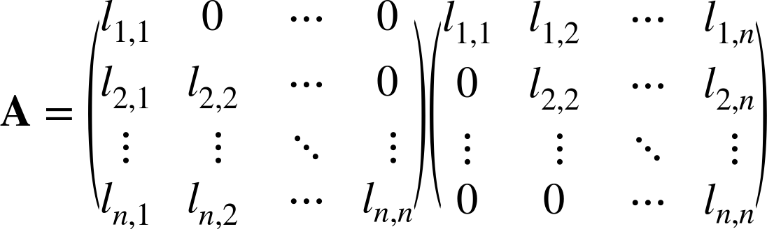
LU Decomposition
The lower-upper (LU) decomposition decomposes a matrix A into a lower diagonal matrix L and an upper diagonal matrix U such that A = LU:

LUDecompositionlud=newLUDecomposition(matrix);RealMatrixu=lud.getU();RealMatrixl=lud.getL();
The LU decomposition is useful in solving systems of linear equations in which the number of unknowns is equal to the number of equations.
QR Decomposition
The QR decomposition decomposes the matrix A into an orthogonal matrix of column unit vectors Q and an upper triangular matrix R such that

QRDecompositionqrd=newQRDecomposition(matrix);RealMatrixq=lud.getQ();RealMatrixr=lud.getR();
One of the main uses of the QR decomposition (and analogous decompositions) is in the calculation of eigenvalue decompositions because each column of Q is orthogonal. The QR decomposition is also useful in solving overdetermined systems of linear equations. This is usually the case for datasets in which the number of data points (rows) is greater than the dimension (number of columns). One advantage of using the QR decomposition solver (as opposed to SVD) is the easy access to the errors on the solution parameters that can be directly calculated from R.
Singular Value Decomposition
The singular value decomposition (SVD) decomposes the m × n matrix A such that A = UΣVT, where U is an m × m unitary matrix, S is an m × n diagonal matrix with real, non-negative values, and V is an n × n unitary matrix. As unitary matrices, both U and V have the property UUT = I, where I is the identity matrix.

In many cases, ![]() ; the number of rows in a matrix will be greater than
or equal to the number of columns. In this case, there is no need to
calculate the full SVD. Instead, a more efficient calculation called
thin SVD can be implemented, where U is m ×
n, S is
n × n, and V is n ×
n. As a practical matter, there may also be cases
when
; the number of rows in a matrix will be greater than
or equal to the number of columns. In this case, there is no need to
calculate the full SVD. Instead, a more efficient calculation called
thin SVD can be implemented, where U is m ×
n, S is
n × n, and V is n ×
n. As a practical matter, there may also be cases
when ![]() so we can then just use the smaller of the two
dimensions:
so we can then just use the smaller of the two
dimensions: ![]() . The Apache Commons Math implementation uses that practice:
. The Apache Commons Math implementation uses that practice:
/* matrix is mxn and p = min(m,n) */SingularValueDecompositionsvd=newSingularValueDecomposition(matrix);RealMatrixu=svd.getU();// m x pRealMatrixs=svd.getS();// p x pRealMatrixv=svd.getV();// p x n/* retrieve values, in decreasing order, from the diagonal of S */double[]singularValues=svd.getSingularValues();/* can also get covariance of input matrix */doubleminSingularValue=0;// 0 or neg value means all sv are usedRealMatrixcov=svd.getCovariance(minSingularValue);
The singular value decomposition has several useful properties. Like the eigen decomposition, it is used to reduce the matrix A to a smaller dimension, keeping only the most useful of them. Also, as a linear solver, the SVD works on any shape of matrix and in particular, is stable on underdetermined systems in which the number of dimensions (columns) is much greater than the number of data points (rows).
Eigen Decomposition
The goal of the eigen decomposition is to reorganize the matrix A into a set of independent and orthogonal column vectors called eigenvectors. Each eigenvector has an associated eigenvalue that can be used to rank the eigenvectors from most important (highest eigenvalue) to least important (lowest eigenvalue). We can then choose to use only the most significant eigenvectors as representatives of matrix A. Essentially, we are asking, is there some way to completely (or mostly) describe matrix A, but with fewer dimensions?
For a matrix A, a solution exists for a vector x and a constant λ such that Ax = λx. There can be multiple solutions (i.e., x, λ pairs). Taken together, all of the possible values of lambda are known as the eigenvalues, and all corresponding vectors are known as the eigenvectors. The eigen decomposition of a symmetric, real matrix A is expressed as A = VDVT. The results are typically formulated as a diagonal m × m matrix D, in which the eigenvalues are on the diagonal and an m × m matrix V whose column vectors are the eigenvectors.

Several methods exist for performing an eigenvalue decomposition.
In a practical sense, we usually need only the simplest form as
implemented by Apache Commons Math in the
org.apache.commons.math3.linear.EigenDecomposition class.
The eigenvalues and eigenvectors are sorted by descending
order of the eigenvalues. In other words, the first eigenvector (the
zeroth column of matrix Q) is the most significant eigenvector.
double[][]data={{1.0,2.2,3.3},{2.2,6.2,6.3},{3.3,6.3,5.1}};RealMatrixmatrix=newArray2DRowRealMatrix(data);/* compute eigenvalue matrix D and eigenvector matrix V */EigenDecompositioneig=newEigenDecomposition(matrix);/* The real (or imag) eigenvalues can be retrieved as an array of doubles */double[]eigenValues=eig.getRealEigenvalues();/* Individual eigenvalues can be also be accessed directly from D */doublefirstEigenValue=eig.getD().getEntry(0,0);/* The first eigenvector can be accessed like this */RealVectorfirstEigenVector=eig.getEigenvector(0);/* Remember that eigenvectors are just the columns of V */RealVectorfirstEigenVector=eig.getV.getColumn(0);
Determinant
The determinant is a scalar value calculated from a matrix A and is most often seen as a component as the multinormal distribution. The determinant of matrix A is denoted as |A|. The Cholesky, eigen, and LU decomposition classes provide access to the determinant:
/* calculate determinant from the Cholesky decomp */doubledeterminant=newCholeskyDecomposition(matrix).getDeterminant();/* calculate determinant from the eigen decomp */doubledeterminant=newEigenDecomposition(matrix).getDeterminant();/* calculate determinant from the LU decomp */doubledeterminant=newLUDecomposition(matrix).getDeterminant();
Inverse
The inverse of a matrix is similar to the concept of inverting a real number ℜ, where
ℜ(1/ℜ) = 1. Note that this can also be written as
ℜℜ–1 = 1. Similarly, the inverse of a matrix
A is denoted by A–1 and the relation
exists AA–1 = I, where I is
the identity matrix. Although formulas exist for directly computing the
inverse of a matrix, they are cumbersome for large matrices and
numerically unstable. Each of the decomposition methods available in
Apache Commons Math implements a DecompositionSolver interface
that requires a matrix inverse in its solution of linear systems. The
matrix inverse is then retrieved from the accessor method of the
DecompositionSolver class. Any of the decomposition methods
provides a matrix inverse if the matrix type is compatible with the method used:
/* the inverse of a square matrix from Cholesky, LU, Eigen, QR,or SVD decompositions */RealMatrixmatrixInverse=newLUDecomposition(matrix).getSolver().getInverse();
The matrix inverse can also be calculated from the singular value decomposition:
/* the inverse of a square or rectangular matrix from QR or SVD decomposition */RealMatrixmatrixInverse=newSingularValueDecomposition(matrix).getSolver().getInverse();
/* OK on rectangular matrices, but error on non-singular matrices */RealMatrixmatrixInverse=newQRDecomposition(matrix).getSolver().getInverse();
A matrix inverse is used whenever matrices are moved from one side of the equation to the other via division. Another common application is in the computation of the Mahalanobis distance and, by extension, for the multinormal distribution.
Solving Linear Systems
At the beginning of this chapter, we described the system XW = Y as a fundamental concept of linear algebra. Often, we
also want to include an intercept or offset term ![]() not dependent on
not dependent on ![]() such that
such that

There are two options for including the intercept term, the first of
which is to add a column of 1s to X and a row of unknowns to W. It does not matter which column-row pair is chosen as
long as ![]() in this case. Here we choose the last column of
X and the last row of W:
in this case. Here we choose the last column of
X and the last row of W:

Note that in this case, the columns of W are independent. Therefore, we are simply finding
![]() separate linear models, except for the convenience of
performing the operation in one piece of code:
separate linear models, except for the convenience of
performing the operation in one piece of code:
/* data */double[][]xData={{0,0.5,0.2},{1,1.2,.9},{2,2.5,1.9},{3,3.6,4.2}};double[][]yData={{-1,-0.5},{0.2,1},{0.9,1.2},{2.1,1.5}};/* create X with offset as last column */double[]ones={1.0,1.0,1.0,1.0};intxRows=4;intxCols=3;RealMatrixx=newArray2DRowRealMatrix(xRows,xCols+1);x.setSubMatrix(xData,0,0);x.setColumn(3,ones);// 4th column is index of 3 !!!/* create Y */RealMatrixy=newArray2DRowRealMatrix(yData);/* find values for W */SingularValueDecompositionsvd=newSingularValueDecomposition(x);RealMatrixsolution=svd.getSolver().solve(y);System.out.println(solution);// {{1.7,3.1},{-0.9523809524,-2.0476190476},// {0.2380952381,-0.2380952381},{-0.5714285714,0.5714285714}}
Given the values for the parameters, the solution for the system of equations is as follows:


The second option for including the intercept is to realize that the preceding algebraic expression is equivalent to the affine transformation of a matrix described earlier in this chapter:

This form of a linear system has the advantage that we do not need to resize any matrices. In the previous example code resizing the matrices occurs only one time, and this is not too much of a burden. However, in Chapter 5, we will tackle a multilayered linear model (deep network) in which resizing matrices will be cumbersome and inefficient. In that case, it is much more convenient to represent the linear model in algebraic terms, where W and b are completely separate.