Chapter
2

Storage Devices

TOPICS COVERED IN THIS CHAPTER:

• Storage from 40,000 feet
• The mechanical disk drive
• Disk drive performance
• Disk drive reliability
• Solid-state media
• Solid-state performance
• Solid-state reliability
• Tape
• Hybrid Drives

This chapter covers everything you will need to know about disk drives and solid-state drives for both your career in IT as well as the CompTIA Storage+ exam.

Because a solid understanding of the disk drive and solid-state technology is so fundamental to a successful career in storage, this chapter covers a lot of the underlying theory in depth. It covers all the major mechanical components of the spinning disk drive as well as diving into the theory and inner workings of flash memory and solid-state technologies. It introduces you to the wildly different performance characteristics of spinning media vs. solid-state media. Each has its place, and it's not necessarily as simple as saying that flash memory and solid-state technologies will totally replace the spinning disk drive.

After you've covered the theory of how these critical data center technologies work, you'll learn a little bit about their impact on overall performance and availability—which will be crucial to your IT environment. You'll also learn about capacities and explore cost-related concepts such as dollars per terabyte ($/TB) and dollars per I/O operation ($/I/O operation) and how these cost metrics can be used to make business cases for storage spending.

Storage from 40,000 Feet

The goal of this chapter is to cover everything that you will ever need to know about the storage devices that dominate data centers across the planet. Those devices are as follows:

• Disk storage
• Solid-state storage
• Tape storage

All three are forms of storage, or media.

Disk storage refers to the electromechanical hard disk drive. But as that is a bit of a mouthful, most people refer to it as a disk drive, hard drive, or hard disk drive (HDD). I'll interchange the terms to keep you on your toes.

Solid-state media refers to a whole bunch of newer technologies that are fighting for a share of the data center oxygen. Many of these are currently flash memory–based, but other forms of solid-state media exist, and many more are on the horizon. This is a particularly exciting area of storage.

Tape storage refers to magnetic tape. As crazy as it may sound, magnetic tape is still found in IT infrastructures across the globe. And like the disk drive, tape shows no signs of giving up its share of the data center oxygen. I expect magnetic tape to outlive me, and I'm planning on a long and happy life.

I think it's worth pointing out that in enterprise tech, when people refer to storage, they are almost always referring to disk or solid-state storage. Occasionally people might use the term to refer to optical media or tape, but nobody ever uses it to refer to memory. It's only the nontech novice who thinks their PC has 1 TB of memory (it really has 1 TB of storage).

Disk, solid-state, and tape storage are all forms of persistent storage, or nonvolatile storage. Both terms mean the same thing: if you throw the power switch off, your data will still be there when you turn the power back on. Of course, you should never just throw the switch on your computer equipment. You need to be careful to turn off the computer in a sensible way, as any data that is only partially written when the power is pulled will be only partially written when the power is restored—a term known as crash consistent. This behavior differs from that of memory, such as DRAM; if you pull the power to DRAM, you can kiss goodbye the data it once stored!

Now that those basics are done with, let's get up close and personal with each of these vital storage technologies.

The Mechanical Disk Drive

Hey, we're well into the 21st century, right? So why are we still rattling on about the mechanical disk drive? It's a hunk of rotating rust that belongs back in the 20th century, right?

Wrong!

Yes, the disk drive is ancient. Yes, it's been around for well over 50 years. And yes, it is being pushed to its limits more than ever before. But like it or lump it, the mechanical disk drive is showing no signs of taking voluntary retirement any time soon.

As the disk drive and its quirky characteristics are absolutely fundamental to a solid understanding of storage, I highly recommend you know the disk drive inside and out. If you don't, it will come back to bite you later. You have been warned!

The Anatomy of a Disk Drive

In the vast majority of servers, laptops, and home PCs, the disk drive is the last remaining mechanical component. Everything else is silicon based. This is important to know, because it makes the disk drive hundreds, sometimes even thousands, of times slower than everything else in a server or PC.

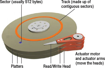
The disk drive is composed of four major mechanical components:

• Platters
• Read/write heads
• Actuator assembly
• Spindle motor

Figure 2.1 shows these components. We will also discuss other components in the following sections.

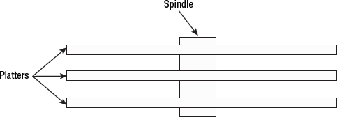
Platter

The platter is where the data is stored. A platter looks just like any other rigid, circular disk such as a Blu-ray Disc or DVD. Most disk drives have several platters stacked above each other, as shown in Figure 2.2.

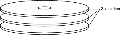
Each platter is rigid (it doesn't bend), thin, circular, insanely flat and smooth, and spins like the wind. Data is read and written to the platter surfaces by the read/write heads, which are controlled by the actuator assembly—more on these later.

Platters are often constructed of a glass or aluminum substrate, and each platter surface is magnetically coated. Both the top and bottom surface of each platter are used to store data. Capacity is so often the name of the game when it comes to disk drives that absolutely no space is wasted, ever!

Because all platters are attached to a common shaft (the spindle), all platters in a disk drive rotate in sync, meaning they all start and stop at the same time and spin at the same speed.

Read/Write Heads

Read/write heads are sometimes referred to as R/W heads, or just heads. These are the babies that fly above the platter surface and read and write data to the platters. They are attached to the actuator assembly and are controlled by the firmware on the disk drive controller. Higher-level systems such as operating systems, volume managers, and filesystems never know anything about R/W heads.

Flying Height

The read/write heads fly at incredibly minute distances above each platter, referred to as flying height. Flying height is measured in nanometers. And if a nanometer doesn't mean anything to you, the flying height of most disk drives is less than the size of a speck of dust or the depth of a fingerprint. Figure 2.3 helps put this in perspective and does a great job of illustrating the precision engineering that goes into the design and manufacturing of the modern disk drive. The disk drive is nothing short of a marvel of modern engineering!

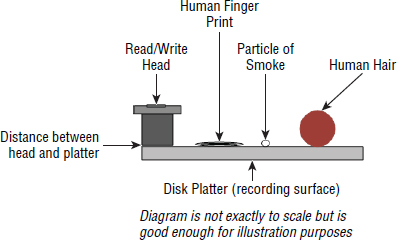
It is not only the flying height of the heads that is extremely microscopic and precise; the positioning of the heads over the correct sector is also ridiculously precise. The data is so densely packed onto the platter surface these days that being out of position by the most minuscule fraction will see the R/W heads reading or writing to the wrong location on disk. That is called corruption, and you don't want to go there!

Head Crashes

It is vital to note that the read/write heads never touch the surface of a platter. If they do touch, this is known as a head crash and almost certainly results in the data on the drive being unreadable and the drive needing replacement.

Reading and Writing to the Platter

As the heads fly over the surface of the platter, they have the ability to sense and alter the magnetic orientation of the bits in the sectors and tracks that pass beneath them.

When writing data, the read/write heads fly above or below each platter surface and magnetize the surface as they pass over it. Magnetic charging is done in a way to represent binary ones and zeros. When reading data from the platter surfaces, the read/write heads detect the magnetic charge of the areas beneath them to determine whether it represents a binary one or zero. There is effectively no limit to the number of times you can read and write a sector of a disk.

Heads and Internal Drive Addressing

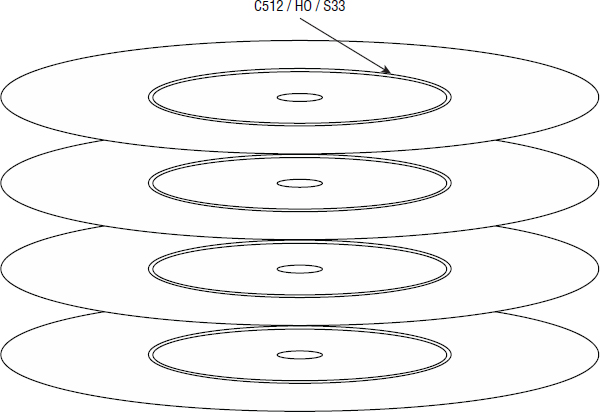
Each platter surface has its own R/W heads. Figure 2.4 shows a drive with three platters and six R/W heads. Each platter has two recording surfaces—top and bottom—and each surface has its own R/W head. Three platters, each with two recording surfaces, equal six recording surfaces. To read and write from these recording surfaces, we need six R/W heads.

This concept of heads and recording surfaces is important in the cylinder-head-sector (CHS) addressing scheme used by disk drives and referenced in the CompTIA Storage+ exam objectives. To address any sector in a disk drive, you can specify the cylinder number (which gives us the track), the head number (which tells us which recording surface this track is on), and the sector number (which tells us which sector on the track we have just identified). Figure 2.5 shows cylinder 512, head 0, sector 33, or put another way, sector 33 on track 512 on platter surface 0.

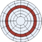
Tracks and Sectors

The surface of every platter is microscopically divided into tracks and sectors. Figure 2.6 shows an example platter divided into tracks and sectors.

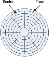
Each platter surface has many tracks, each a concentric ring running all the way around the platter. Each track is then divided into sectors.

The sector is the smallest addressable unit of a disk drive and is typically 512 or 520 bytes in size (we'll work predominantly with 512 bytes in our examples). So, if you want to write only 256 bytes to your disk, you need a whole 512-byte sector and will waste 256 bytes. But don't stress over this; the values are so small as to be insignificant! If you want to write 1,024 bytes, you need four sectors. Simple!

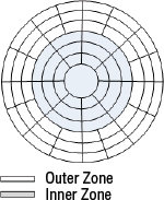
As you can see in Figure 2.6, the physical size of each sector gets smaller and smaller toward the center of the platter. Because each sector stores the same amount of data (for example, 512 bytes), the outer tracks contain wasted space. Wasting space/capacity in disk drive design is a cardinal sin, so a fix had to be invented. To make better use of available space, most modern disks implement a system known as zoned data recording (ZDR): more sectors are squeezed onto tracks closer to the edges than they are on the inner tracks, allowing the drive to store more data. See Figure 2.7 for a graphical depiction.

In ZDR-style disks—and just about every disk in the world implements some form of ZDR—each platter is divided into zones. Tracks in the same zone have the same number of sectors per track. However, tracks in different zones will have a different number of sectors per track.

Figure 2.7 shows a platter surface divided into two zones: the outer zone with 16 sectors per track, and the inner zone with 8 sectors per track. In this simplified example, our platter has three tracks in the outer zone and three tracks in the inner zone, for a total of 72 sectors. If the platter had only a single zone with 8 sectors per track, the same disk would have only 48 sectors, or two-thirds of the potential capacity. Clearly, this is an oversimplified example; in the real world, each track has many more sectors. Even so, this example shows how implementing ZDR techniques can yield greater space efficiencies.

Here are a couple of quick points on performance that are relative to tracks and sectors:

• Because the outer tracks of a platter contain more sectors, it stands to reason they can store and retrieve more data for every spin of the disk. Let's look at a quick example. In our example platter in Figure 2.7, the outer tracks can read or write 16 sectors per rotation, whereas the inner tracks can read or write only 8 sectors per rotation. The outer tracks can perform up to twice as fast as the inner tracks. For this reason, most disk drives will start writing data to the outer tracks of each platter. While this is important theory to know, there is precious little you can do to influence this behavior or exploit your knowledge of it in the real world. My advice is to understand the theory but don't lose any sleep over it!
• If data can be read or written to contiguous sectors on the same or adjacent tracks, you will get better performance than if the data is scattered randomly over the platter. For example, reading sectors 0–15 in the outer track (known as a sequential read) could be accomplished in a single rotation of the platter. In contrast, if the 16 sectors being read were scattered all over the platter surface, the read operation (in this case called a random read) would almost certainly require more than a single rotation. This can be pretty darn important in real life!

This process of dividing a platter into tracks and sectors is done via a factory format.

Each track on a disk has an index marker that allows the read/write heads to maintain accurate positioning—just like lines separating lanes on a highway. Adjacent sectors are separated by servo signals that assist in keeping the R/W heads “on track.”

While sectors have historically been either 512 bytes or 520 bytes, some more modern disk drives are being formatted with larger sector sizes, such as the increasingly popular Advanced Format standard. Larger sector sizes, currently 4K, offer potentially more capacity as they can implement more-efficient integrity checks such as error correction code (ECC). Figure 2.8 compares a 4K Advanced Format drive with a standard drive formatted with 512-byte sectors.

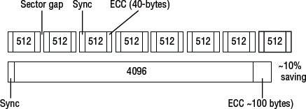
In Figure 2.8, the 512-byte format drive requires 320 bytes of ECC, whereas the 4K formatted drive requires only about 100 bytes. Specifics will change and be improved, but this highlights the potential in using larger sectors.

Interestingly, 4K is something of a magic number in x86 computing. Memory pages are usually 4K, and filesystems are often divided into 4K extents or clusters.

The type of disk where the sector size is preset and cannot be changed is referred to in the industry as fixed block architecture (FBA). This term is rarely used these days, though, as these are the only type of disks you can buy in the open systems world.

Cylinders

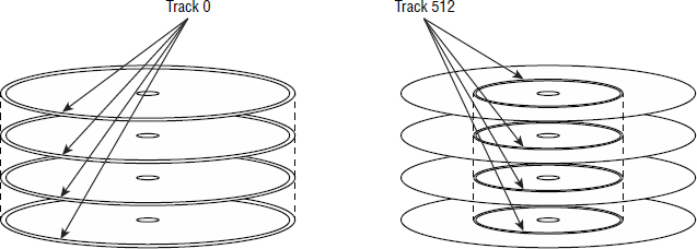
A cylinder is a collection of tracks stacked directly above one another on separate platters. As an example, let's assume our disk drive has four platters, each with two recording surfaces, giving us a total of eight recording surfaces. Each recording surface has the same number of tracks, numbered from track 0 on the outside to track 1,023 on the inside (this is just an example for illustration purposes). Track 0 on each of the eight recording surfaces is the outer track. Track 0 on recording surface 0 is directly above track 0 on all seven other recording surfaces.

This concept is shown in Figure 2.9. On the left is a four-platter disk drive with track 0, the outermost track, highlighted. The platters’ track 0s form a cylinder that we could call cylinder 0. On the right in Figure 2.9 we have the same four-platter drive, this time with track 512 highlighted, and these tracks combine to form cylinder 512.

Logical Block Addressing

The way in which data is stored and retrieved from disk can be pretty complex and can vary massively from one disk to another, depending on the characteristics of the disk—sector size, number of platters, number of heads, zones, and so on. To hide these complexities from the likes of operating systems, disk drives implement what is known as logical block addressing (LBA).

Logical block addressing, implemented in the drive controller of every disk drive, exposes the capacity of the disk as a simplified address space—and it is a godsend! Consider our example platter shown previously in Figure 2.7, with two zones and 72 sectors per platter. Let's assume our drive has four platters, giving us a total of eight recording surfaces (eight R/W heads). The locations on our disk drive will be addressed internally in the disk by a CHS address such as these:

• Cylinder 0, head 0, sector 6
• Cylinder 3, head 6, sector 2
• Cylinder 2, head 0, sector 70

This is ugly, complicated, and specific to each drive type. LBA addressing, on the other hand, couldn't be simpler. The LBA map exposed by the disk controller may simply present a range of 72 logical blocks addressed as LBA0 through LBA71. That's it! Operating systems and filesystems just address reads and writes to LBA addresses without understanding the underlying layout of the disk drive, and the controller on the disk drive takes care of the exact CHS address.

While this might not seem to be very much, consider that all modern disk drives have multiple platters, each with two recording surfaces, and each surface with its own read/write head. You can see how this could quickly become complicated.

Interestingly, because all open-systems operating systems and volume managers work with LBAs, they never know the precise location of data on disk! Only the disk controller knows this, as it owns the LBA map. Sound worrying? It shouldn't; the LBA scheme has been used safely and successfully for many years. Figure 2.10 shows how CHS addresses are mapped to LBA addresses on the disk drive controller.

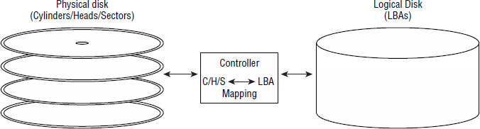
A major advantage of the LBA scheme implemented by intelligent disk controllers is that operating system drivers for disks have been hugely simplified and standardized. When was the last time you had to install a custom driver for a newly installed disk drive? The OS/driver can simply issue read/write requests, specifying LBA addresses, to the disk, and the controller converts these commands and locations into the more primitive seek, search, read and write commands, as well as CHS locations.

Actuator Assembly

The next important physical component in every disk drive is the actuator assembly. Each disk drive has a single actuator assembly, and it is the job of that assembly to physically move the R/W heads (under the direction of the disk drive firmware and controller). And when I say move them, I mean move them! If you haven't seen R/W heads flicking back and forth over the surface of a platter, you haven't lived! They move fast and with insane precision. Because a disk drive has only a single actuator, all heads (one for each platter surface) move in unison.

Spindle

Every platter in a disk drive is connected to the spindle, and it is the job of the spindle and spindle motor to spin the disks (platters). See Figure 2.11. Each disk drive has only a single spindle, and the speed at which the spindle motor spins the platters is amazingly fast, and again, amazingly precise.

The center of each platter is attached to the spindle, and when the spindle spins, so do the platters. Because there is a single spindle and all platters attach to it, all platters start and stop spinning at the same time—when the spindle starts and stops. Each platter therefore spins at the same velocity, known as revolutions per minute (RPM).

Controller

Each disk drive comes with its own controller. This controller is like a mini computer just for the disk drive. It has a processor and memory, and it runs firmware that is vital to the operation of the drive.

It is the controller that masks the complexities of the physical workings of the disk and abstracts the layout of data on the drive into the simpler LBA form that is presented up to the higher levels such as the BIOS and OS. Higher levels such as the OS are able to issue simple commands such as read and write to the controller, which then translates them into the more complex operations native to the disk drive. The controller firmware also monitors the health of the drive, reports potential issues, and maintains the bad block map.

Interfaces and Protocols

A protocol can easily be thought of as a set of commands and rules of communication. Disk drives, solid-state media, and storage arrays speak a protocol. (Disk arrays often speak multiple protocols.) However, in the storage world, each protocol often has its own physical interface specifications as well, meaning that protocol can also relate to the physical interface of a drive. For example, a SATA drive speaks the SATA protocol and also has a physical SATA interface. The same goes for SAS and FC; each has its own interface and protocol.

The four most common protocols and interfaces in the disk drive world are as follows:

• Serial Advanced Technology Attachment (SATA)
• Serial Attached SCSI (SAS)
• Nearline SAS (NL-SAS)
• Fibre Channel (FC)

All of these are both a protocol and a physical interface specification. Of the latter two, the underlying command set is SCSI, whereas with SATA the underlying command set is ATA. These protocols are implemented on the disk controller and determine the type of physical interface in the drive.

SATA

SATA has its roots in the low end of the computing market such as desktop PCs and laptops. From there, it has muscled its way into the high-end enterprise tech market, but it is quickly being replaced in storage arrays by NL-SAS.

In enterprise tech, SATA drives are synonymous with cheap, low performance, and high capacity. The major reason for this is that the ATA command set is not as rich as the SCSI command set, and as a result not as well suited to high-performance workloads. Consequently, disk drive vendors implement SATA drives with lower-cost components, smaller buffers, and so on.

However, the enterprise tech world is not all about high performance. There is absolutely a place for low-cost, low-performance, high-capacity disk drives. Some examples are backup and archiving appliances, as well as occupying the lower tiers of auto-tiering solutions in storage arrays. However, most of these requirements are now satisfied by NL-SAS drives rather than SATA.

SAS

SAS is, as the name suggests, a serial point-to-point protocol that uses the SCSI command set and the SCSI advanced queuing mechanism. SCSI has its roots firmly in the high-end enterprise tech world, leading to it have a richer command set, better queuing system, and often better physical component quality than SATA drives. All this tends to make SCSI-based drives, such as SAS and FC, the best choice for high-performance, mission-critical workloads.

Of course, performance comes at a cost. SAS drives are more expensive than SATA drives of similar capacity.

Another key advantage of SAS is that SATA II, and newer, drives can connect to a SAS network or backplane and live side by side with SAS drives. This makes SAS a flexible option when building storage arrays.

SAS drives are also dual ported, making them ideal for external storage arrays and adding higher resilience. On the topic of external storage arrays and SAS drives, each port on the SAS drive can be attached to different controllers in the external storage array. This means that if a single port, connection to the port, or even the controller fails, the drive is still accessible over the surviving port. This failover from the failed port to the surviving port can be fast and transparent to the user and applications. Although SAS drives are dual ported, these ports work in an active/passive mode, meaning that only one port is active and issuing commands to the drive at any one point in time.

Finally, SAS drives can be formatted with arbitrary sector sizes, allowing them to easily implement EDP (sometimes called DIF). With EDP, 520-bye sectors are used instead of 512-bye sectors. The additional 8 bytes per sector are used to store metadata that can ensure the integrity of the data, making sure that it hasn't become corrupted.

FC

FC drives implement the SCSI command set and queuing just like SAS, but have dual FC-AL or dual FC point-to-point interfaces. They too are suited to high-performance requirements and come at a relatively high cost per gigabyte, but are very much being superseded by SAS drives.

NL-SAS

Nearline SAS (NL-SAS) drives are a hybrid of SAS and SATA drives. They have a SAS interface and speak the SAS protocol, but also have the platters and RPM of a SATA drive.

What's the point? Well, they slot easily onto a SAS backplane or connector and provide the benefits of the SCSI command set and advanced queuing, while at the same time offering the large capacities common to SATA. All in all, it is a nice blend of SAS and SATA qualities.

NL-SAS has all but seen off SATA in the enterprise storage world, with all the major array vendors supporting NL-SAS in their arrays.

Queuing

All disk drives implement a technique known as queuing. Queuing has a positive impact on performance.

Queuing allows the drive to reorder I/O operations so that the read and write commands are executed in an order optimized for the layout of the disk. This usually results in I/O operations being reordered so that the read and write commands can be as sequential as possible so as to inflict the least head movement and rotational latency as possible.

The ATA command set implements Native Command Queuing (NCQ). This improves the performance of the SATA drive, especially in concurrent IOPS, but is not as powerful as its cousin Command Tag Queuing in the SCSI world.

Drive Size

In the storage world, size definitely matters! But it also matters that you know what you're talking about when it comes to disk size.

When speaking of disk drives, there are two types of size you need to be aware of:

• Capacity
• Physical form factor

Normally, when referring to the size of a drive, you are referring to its capacity, or how much data it can store. Back in the day, this was expressed in megabytes (MB) but these days we tend to talk in gigabytes (GB) or terabytes (TB). And if you really want to impress your peers, you talk about the multipetabyte (PB) estate that you manage!

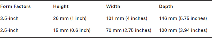
However, the size of a drive can also refer to the diameter of the drive's platter, which is normally referred to as the drive's form factor. In modern disk drives, there are two popular HDD form factors:

• 3.5-inch
• 2.5-inch

As you might expect, a drive with a 2.5-inch platter is physically smaller than a drive with a 3.5-inch platter. And as you may also expect, more often than not, a 3.5-inch drive can store more data than a 2.5-inch drive. This is simple physics; a 3.5-inch platter has more surface area on which to record data.

All 3.5-inch drives come in the same-size casing, meaning that all 3.5-inch drives can fit in the same slots in a server or disk array. The same goes for 2.5-inch drives. All 2.5-inch drives come in the same-size casing, meaning that any 2.5-inch drive can be swapped out and replaced by another. So even though technically speaking, 2.5-inch and 3.5-inch refer to the diameter of the platter, more often than not when we refer to the physical dimensions of one of these drives, we are referring to the size of the casing that it comes in. Table 2.1 shows the measurements of each of these two form factors.

Interestingly, solid-state drive manufacturers have been quick to adopt the common 2.5-inch and 3.5-inch form factors. This can be good, because it makes it as simple as possible to use solid-state drive (SSD) instead of mechanical disk.

Usable Capacity

While speaking about capacity, it is worth pointing out that you don't typically get what it says on the tin when you buy a disk drive. For example, when buying a 900 GB drive, you almost certainly won't get 900 GB of usable space from that drive. There are several reasons for this.

One reason is that storage capacities can be expressed as either base 10 (decimal) or base 2 (binary). As an example, 1 GB is slightly different in base 10 than in base 2:

As you can imagine, when we're talking about a lot of gigabytes, or even terabytes, the difference between the two numbers can become significant:

In this TB example, the difference is just over 9 GB!

If the drive manufacturer quotes in base 2 but your OS quotes in base 10, you can see how you might feel as though you've been shortchanged.

Other factors play into this as well. For example, when formatting a disk in an OS, the OS and filesystem often consume some space as overhead. Similarly, when installing a disk in a storage array, the array will normally shave off some capacity as overhead.

There is also RAID and other things to consider. The bottom line is, don't be surprised if you get slightly less than you bargained for.

Drive Speed

Now that you know what capacity and form factor refer to, let's move on to drive speed. Drive speed is all about how fast the platters spin—and they spin really fast! But instead of a metric such as miles per hour, drive speed is expressed as revolutions per minute (RPM). Simply put, this is how many times the platter spins every minute.

The common drive speeds are as follows:

• 5,400 RPM
• 7,200 RPM
• 10,000 RPM
• 15,000 RPM

These are usually shortened to 5.4K, 7.2K, 10K, and 15K, respectively.

If RPM doesn't do it for you, look at it like this: a 3.5-inch platter spinning at 15,000 RPM is moving at over 150 mph (or about 240 kilometers per hour) at the outer edges. That's what I'm talking about!

RPM converts directly into drive performance. More RPMs = more performance (and higher price, of course).

There is also a strong correlation between RPM and capacity. Usually, the higher the RPM of a drive, the lower the capacity of that drive. Conversely, the lower the RPM of a drive, the higher the capacity.

Another point worth noting is that 10K and 15K drives usually implement the SCSI command set and have a SAS or FC interface. So, faster drives implement the more performance-tuned protocol and interface. That makes sense. Also, the 5.4K and 7.2K drives usually implement the ATA command set and have a SATA interface.

If you've been reading this from the start, the following should now make perfect sense:

Now that you're familiar with the anatomy and major characteristics of disk drives, let's look at how everything comes together in the performance of a drive.

Disk Drive Performance

Several factors influence disk drive performance, and the following sections cover the more important ones. We've already touched on some of these, but we will go in to more detail now.

Two major factors influence disk drive performance:

• Seek time
• Rotational latency

Both of these fall into the category of positional latency—basically, anything that requires the heads to move or wait for the platter to spin into position. Because these are mechanical operations, the delays that these operations introduce can be significant.

Let's take a closer look at each of them before moving on to some of the other disk drive performance considerations, such as IOPS and transfer rate.

Seek Time

Seek time is the time taken to move the read/write heads to the correct position on disk (positioning them over the correct track and sector). Faster is better, and as seek time is expressed in milliseconds (ms), the lower the number, the better.

Seek time can therefore have a significant impact on random workloads, and excessive seeking is often referred to as head thrashing or sometimes just thrashing. And thrashing absolutely kills disk drive performance!

On very random, small-block workloads, it is not uncommon for the disk to spend over 90 percent of its time seeking. As you can imagine, this seriously slows things down! For example, a disk may achieve along the lines of 100 MBps with a nice sequential workload, but give it a nasty random workload, and you could easily be down to less than a single MBps!

Some real-world average seek times taken from the spec sheets of different RPM drives are listed here:

• 15K drive: 3.4/3.9 ms
• 7.2K drive: 8.5/9.5 ms

In this list, the first number on each line is for reads, and the second number is for writes.

Rotational Latency

Rotational latency is the other major form of positional latency. It is the time it takes for the correct sector to arrive under the R/W head after the head is positioned on the right track.

Rotational latency is directly linked to the RPM of a drive. Faster RPM drives have better rotational latency (that is, they have less rotational latency). While seek time is significant in only random workloads, rotational latency is influential in both random and sequential workloads.

Disk drive vendors typically list rotational latency as average latency and express it in milliseconds. Average latency is accepted in the industry as the time it takes for the platter to make a half rotation (that is, spin halfway around). Following are a couple of examples of average latency figures quoted from real-world disk drive spec sheets:

• 15K drive = 2.0 ms
• 7.2K drive = 4.16 ms

Understanding IOPS

IOPS is an acronym for input/output operations per second and is pronounced eye-ops. IOPS is used to measure and express performance of mechanical disk drives, solid-state drives and storage arrays. As a performance metric, IOPS is most useful at measuring the performance of random workloads such as database I/O.

Unfortunately, IOPS is probably the most used and abused storage performance metric. Vendors, especially storage array vendors, are often far too keen to shout about insanely high IOPS numbers in the hope that you will be so impressed that you can't resist handing your cash over to them in exchange for their goods. So, take storage array vendor IOPS numbers with a large grain of salt! Don't worry, though. By the end of this section, you should have enough knowledge to call their bluff.

So what is an I/O operation? An I/O operation is basically a read or a write operation that a disk or disk array performs in response to a request from a host (usually a server).

If only it were that simple! Unfortunately, there are several types of I/O operations. Here are the most important:

• Read
• Write
• Random
• Sequential
• Cache hit
• Cache miss

To further complicate matters, the size of the I/O operation also makes a big difference.

Read and Write IOPS

Read and write IOPS should be simple to understand. You click Save on the document you are working on, and your computer saves that file to disk via one or more write IOPS. Later when you want to open that document to print it, your computer reads it back from disk via one or more read IOPS.

Random vs. Sequential IOPS

As you already know, mechanical disk drives thrive on sequential workloads but hunt like a lame dog when it comes random workloads. There isn't much you can do about that without getting into complicated configurations that are pointless in a world where solid state is so prevalent.

Solid-state media, on the other hand, loves random workloads and isn't at its best with sequential workloads. Let's take a quick look at a massively oversimplified, but useful, example showing why disk drives like sequential workloads so much more than random.

Figure 2.12 shows a simple overhead view of a disk drive platter. A single track (track 2, which is the third track from the outside because computers count tracks starting with 0, not 1) is highlighted with sixteen sectors (0–15).

A sequential write to eight sectors on that track would result in sectors 0–7 being written to in order. This could be accomplished during a single rotation of the disk—remember that disks rotate thousands of times per minute. If that same data needed to be read back from disk, that read operation could also be satisfied by a single rotation of the disk. Not only will the disk have to rotate only once, but the read/write heads will not have to perform any seeking. So you have zero positional latency. However, there will still likely be some rotational latency while we wait for the correct sectors to arrive under the R/W heads. Nice!

Now let's assume a random workload. To keep the comparison fair, we will read or write another eight sectors’ worth of data and we will stick to just track 2 as in our previous example. This time, the sectors need to be read in the following order: 5, 2, 7, 8, 4, 0, 6, 3. If the R/W head starts above sector 0, this read pattern will require five revolutions of the disk:

This results in a lot more work and a lot more time to service the read request! And remember, that example is painfully simplistic. Things get a whole lot more complicated when we throw seeking into the mix, not to mention multiple platters!

Cache Hits and Cache Misses

Cache-hit IOPS, sometimes referred to as cached IOPS¸ are IOPS that are satisfied from cache rather than from disk. Because cache is usually DRAM, I/O operations serviced by cache are like greased lightning compared to I/O operations that have to be serviced from disk.

When looking at IOPS numbers from large disk-array vendors, it is vital to know whether the IOPS numbers being quoted are cache hits or misses. Cache-hit IOPS will be massively higher and more impressive than cache-miss IOPS. In the real world, you will have a mixture of cache hit and cache miss, especially in read workloads, so read IOPS numbers that are purely cache hit are useless because they bear no resemblance to the real world. Statements such as 600,000 IOPS are useless unless accompanied by more information such as 70% read, 30% write, 100% random, 4K I/O size, avoiding cache.

Calculating Disk Drive IOPS

A quick and easy way to estimate how many IOPS a disk drive should be able to service is to use this formula:

where x = average seek time, and y = average rotational latency

A quick example of a drive with an average seek time of 3.5 ms and an average rotational latency of 2 ms gives us an IOPS value of 181 IOPS:

This works only for spinning disks and not for solid-state media or disk arrays with large caches.

MBps

Megabytes per second (MBps) is another performance metric. This one is used to express the number of megabytes per second a disk drive or storage array can perform. If IOPS is best at measuring random workloads, MBps is most useful when measuring sequential workloads such as media streaming or large backup jobs.

Maximum and Sustained Transfer Rates

Maximum transfer rate is another term you'll hear in reference to disk drive performance. It is usually used to express the absolute highest possible transfer rate of a disk drive (throughput or MBps) under optimal conditions. It often refers to burst rates that cannot be sustained by the drive. Take these numbers with a pinch of salt. A better metric is sustained transfer rate (STR).

STR is the rate at which a disk drive can read or write sequential data spread over multiple tracks. Because it includes data spread over multiple tracks, it incorporates some fairly realistic overheads, such as R/W head switching and track switching. This makes it one of the most useful metrics for measuring disk drive performance.

The following is an example of the differences between maximum transfer rate and sustained transfer rate from a real-world disk drive spec sheet for a 15K drive:

• Maximum: 600 MBps
• Sustained: 198 MBps

Disk Drive Reliability

There is no doubt that disk drives are far more reliable than they used to be. However, disk drives do fail, and when they fail, they tend to catastrophically fail. Because of this, you absolutely must design and build storage solutions with the ability to cope with disk drive failures.

It is also worthy of note that enterprise-class drives are more reliable than cheaper, consumer-grade drives. There are a couple of reasons:

• Enterprise-class drives are often made to a higher specification with better-quality parts. That always helps!
• Enterprise drives tend to be used in environments that are designed to improve the reliability of disk drives and other computer equipment. For example, enterprise-class disk drives are often installed in specially designed cages in high-end disk arrays. These cages and arrays are designed to minimize vibration, and have optimized air cooling and protected power feeds. They also reside in data centers that are temperature and humidity controlled and have extremely low levels of dust and similar problems. Compare that to the disk drive in that old PC under your desk!

Mean Time between Failure

When talking about reliability of disk drives, a common statistic is mean time between failure, or MTBF for short. It is an abomination of a statistic that can be hideously complicated and is widely misunderstood. To illustrate, a popular 2.5-inch 1.2 TB 10K SAS drive states a MTBF value of 2 million hours! This absolutely does not mean that you should bank on this drive running for 228 years (2 million hours) before failing. What the statistic might tell you is that if you have 228 of these disk drives in your environment, you could expect to have around one failure in the first year. Aside from that, it is not a useful statistic.

Annualized Failure Rate

Another reliability specification is annual failure rate (AFR). This attempts to estimate the likelihood that a disk drive will fail during a year of full use. The same 1.2 TB drive in the preceding example has an AFR of less than 1 percent.

With all of this statistical mumbo jumbo out of the way, the cold, hard reality is that disk drives fail. And when they fail, they tend to fail in style—meaning that when they die, they usually take all their data with them! So you'd better be prepared! This is when things like RAID come into play. RAID is discussed in Chapter 4, “RAID: Keeping Your Data Safe.”

Solid-State Media

Let's leave all that mechanical stuff behind us and move on to the 21st century. The field of solid-state media is large, exciting, and moving at an amazing pace! New technologies and innovations are hitting the street at an incredible rate. Although solid-state media, and even flash memory, have been around for decades, uptake has been held back because of capacity, reliability, and cost issues. Fortunately for us, these are no longer issues, and solid-state storage is truly taking center stage.

I should probably start by saying that solid-state media comes in various shapes and sizes. But these are the two that we are most interested in:

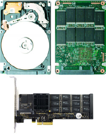
Solid-State Drive (SSD) For all intents and purposes, an SSD looks and feels like a hard disk drive (HDD). It comes in the same shape, size, and color. This means that SSDs come in the familiar 2.5- and 3.5-inch form factors and sport the same SAS, SATA, and FC interfaces and protocols. You can pretty much drop them into any system that currently supports disk drives.

PCIe Card/Solid-State Card (SSC) This is solid-state media in the form of a PCI expansion card. In this form, the solid-state device can be plugged into just about any PCIe slot in any server or storage array. These are common in servers to provide extremely high performance and low latency to server apps. They are also increasingly popular in high-end storage arrays for use as level 2 caches and extensions of array caches and tiering.

Figure 2.13 shows a mechanical drive side by side with a solid state drive, and a PCIe solid-state device beneath. The HDD and SSD are to scale, but the PCIe card is not.

There are also different types of solid-state media, such as flash memory, phase-change memory (PCM), memristor, ferroelectric RAM (FRAM), and plenty of others. However, this chapter focuses on flash memory because of its wide adoption in the industry. Other chapters cover other technologies when discussing the future of storage.

Unlike a mechanical disk drive, solid-state media has no mechanical parts. Like everything else in computing, solid-state devices are silicon/semiconductor based. Phew! However, this gives solid-state devices massively different characteristics and patterns of behavior than spinning disk drives. The following are some of the important high-level differences:

• Solid state is the king of random workloads, especially random reads!
• Solid-state devices give more-predictable performance because of the total lack of positional latency such as seek time.
• Solid-state media tends to require less power and cooling than mechanical disk.
• Sadly, solid-state media tends to come at a much higher $/TB capital expenditure cost than mechanical disk.

Solid-state devices also commonly have a small DRAM cache that is used as an acceleration buffer as well as for storing metadata such as the block directory and media-related statistics. They often have a small battery or capacitor to flush the contents of the cache in the event of sudden power loss.

No More RPM or Seek Time

Interestingly, solid-state media has no concept of positional or mechanical delay. There is obviously no rotational latency because there is no spinning platter, and likewise there is no seek time because there are no R/W heads. Because of this, solid-state media wipes the floor with spinning disks when it comes to random workloads. This is especially true of random reads, where solid-state performance is often closer to that of DRAM than spinning disk. This is nothing short of game changing!

Flash Memory

Flash memory is a form of solid-state storage. By that, I mean it is semiconductor based, has no moving parts, and provides persistent storage. The specific type of flash memory we use is called NAND flash, and it has a few quirks that you need to be aware of. Another form of flash memory is NOR flash, but this is not commonly used in storage and enterprise tech.

Writing to Flash Memory

Writing to NAND flash memory is particularly quirky and is something you need to make sure you understand.

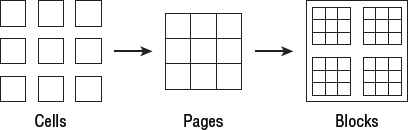
Here is a quick bit of background first. Flash memory is made up of flash cells that are grouped into pages. Pages are usually 4K, 8K, or 16K in size. These pages are then grouped into blocks that are even bigger, often 128K, 256K, or 512K. See Figure 2.14.

A brand new flash device comes with all cells set to 1. Flash cells can be programmed only from a 1 to a 0. If you want to change the value of the cell back to a 1, you need to erase it via a block-erase operation. Now for the small print: erasing flash memory can be done only at a block level! Yes, you read that right. Flash memory can be erased only at the block level. And as you may remember, blocks can be quite large. If you are new to flash, I recommend you read this paragraph again so that it sinks in.

This quirky way of programming/writing to flash means a couple of important things:

• The first time you write to a flash drive, write performance will be blazingly fast. Every cell in the block is preset to 1 and can be individually programmed to 0. There's nothing more to it. It is simple and lightning quick, although still not as fast as read performance.
• If any part of a flash memory block has already been written to, all subsequent writes to any part of that block will require a much more complex and time-consuming process. This process is read/erase/program. Basically, the controller reads the current contents of the block into cache, erases the entire block, and writes the new contents to the entire block. This is obviously a much slower process than if you are writing to a clean block. Fortunately, though, this shouldn't have to occur often, because in a normal operating state a flash drive will have hidden blocks in a pre-erased condition that it will redirect writes to. Only when a flash device runs out of these pre-erased blocks will it have to revert to performing the full read/erase/program cycle. This condition is referred to as the write cliff.

Why does it work like this? Economics! This process requires fewer transistors and significantly reduces manufacturing costs. And it's all about the money!

So to recap, as this may be new to you: The first time you write to a flash memory block, you can write to an individual cell or page, and this is fast. However, once you have changed a single cell in a block, any subsequent update to any cell in that block will be a lot slower because it will require a read/erase/program operation. This is a form of write amplification, which is discussed further later in the chapter.

The Anatomy of NAND Flash

Let's return to the topic of cells, pages, and blocks. This is obviously massively different from the cylinders, heads, and sectors of a spinning disk. Fortunately, flash and other solid-state controllers present the familiar LBA-style view of their contents to the wider world. This means that operating systems, drivers, and volume managers don't need to worry about these low-level differences.

You need to know about four major types of NAND flash:

• Single-level cell (SLC)
• Multi-level cell (MLC)
• Enterprise MLC (eMLC)
• Triple-level cell (TLC)

Each has its pros and cons, as you will see.

Single-Level Cell

In the beginning was single-level cell (SLC). In the SLC world, a single flash cell can store 1 bit of data; the electrical charge applied to the cell could be either on or off (so you can have either binary 0 or binary 1). Figure 2.15 shows an SLC flash cell.

Of the three flash cell options available, SLC provides the highest performance and the longest life span. However, it is also the most expensive and provides the lowest density/capacity.

As a result of SLC's high performance and good write endurance, it is well suited for high-end computing applications. The sad thing is, the world doesn't care too much about the high-end computing market. It isn't big enough to make a lot of money from. The world cares about consumer markets. As a result, there is less and less SLC flash out there. And as it has the highest $/GB cost, maybe it's not so bad that it is going away. Although it is true that SLC is the least power hungry of the flash cell options, this isn't a significant factor in the real world.

Multi-Level Cell

Multi-level cell (MLC) stores 2 bits of data per flash cell (00, 01, 10, or 11), allowing it to store twice as much data per flash cell as SLC does. Brilliant!

Well, it is brilliant from a capacity perspective at least. It is less brilliant from a performance and write endurance perspective. Transfer rates are significantly lower, and P/E cycles are commonly in the region of 10,000 rather than the 100,000 you get from SLC. However, from a random-read performance perspective, it is still way better than spinning disk! MLC has trampled all over the SLC market to the point where MLC is predominant in high-end computing and storage environments.

Interestingly, MLC is able to store 2 bits per flash cell by applying different levels of voltage to a cell. So rather than the voltage being high or low, it can be, high, medium-high, medium-low, or low. This is shown in Figure 2.16.

Enterprise-Grade MLC

Enterprise-grade MLC flash, known more commonly as eMLC, is a form of MLC flash memory with stronger error correction, and therefore lower error rates, than standard MLC flash.

Flash drives and devices based on eMLC technology also tend to be heavily overprovisioned and sport a potentially higher spec flash controller and more intelligence in the firmware that runs on the controller. As an example, a 400 GB eMLC drive might actually have 800 GB of eMLC flash but be hiding 400 GB in order to provide higher performance and better overall reliability for the drive.

On the performance front, eMLC uses the technique of overprovisioning (discussed later in the chapter) to redirect write data to pre-erased cells in the hidden area. These cells can be written to faster than cells that would have to go through the read/program/erase cycle.

On the reliability front, the eMLC drive is able to balance write workload over 800 GB of flash cells rather than just 400 GB, halving the workload on each flash cell and effectively doubling the life of the drive.

Triple-Level Cell

Triple-level cell (TLC) is 100 percent consumer driven, and can be made useful only in enterprise-class computing environments via highly sophisticated methods of smoke and mirrors. Applying complicated firmware and providing massive amounts of hidden capacity creates the illusion that the underlying flash is more reliable than it really is.

I'm sure you've guessed it: TLC stores 3 bits per cell, giving the following binary options: 000, 001, 010, 011, 100, 101, 110, 111. And as you might expect, it also provides the lowest throughput and lowest write endurance levels. Write endurance for TLC is commonly around 5,000 P/E cycles or lower.

So, TLC is high on capacity and low on performance and reliability. That is great for the consumer market, but not so great for the enterprise tech market. Figure 2.17 shows a TLC flash cell.

Flash Overprovisioning

You might come across the terms enterprise-grade flash drives and consumer-grade flash drives. Generally speaking, the quality of the flash is the same. The major difference is usually that the enterprise stuff has a boat load of hidden capacity that the controller reserves for rainy days. This is a technique known as overprovisioning. A quick example is a flash drive that has 240 GB of flash capacity, but the controller advertises only 200 GB as being available. The hidden 40 GB is used by the controller for background housekeeping processes such as garbage collection and static-wear leveling. This improves performance as well as prolongs the life of the device. In these situations, the drive vendor should always list the capacity of the drive as 200 GB and not 240 GB.

Garbage Collection

Garbage collection is a background process performed by the solid-state device controller. Typically, garbage collection involves cleaning up the following:

• Blocks that have been marked for deletion
• Blocks that are only sparsely filled

Blocks that have been marked for deletion can be erased in the background so that they are ready to receive writes without having to perform the dreaded read/erase/program cycle (write amplification). This obviously improves write performance.

Sparsely populated blocks can be combined into fewer blocks, releasing more blocks that can be erased and ready for fast writes. For example, three blocks that are only 30 percent occupied can be combined and reduced to a single block that will be 90 percent full, freeing up two blocks in the process.

These techniques improve performance and elongate the life of the device. However, it is a fine balance between doing too much or too little garbage collection. If you do too much, you inflict too many writes to the flash cells and unnecessarily use up precious P/E cycles for background tasks. If you do too little garbage collection, performance can be poor.

Write Amplification

Write amplification occurs when the number of writes to media is higher than the number of writes issued by the host. A quick example is when a 4K host writes to a 256K flash block that already contains data. As you learned earlier, any write to a block that already contains data requires the following procedure:

1. Read the existing contents of the block into cache.
2. Erase the contents of the block.
3. Program the new contents of the entire block.

This will obviously result in more than a 4K write to the flash media.

Write amplification slows flash performance and unnecessarily wears out the flash cells. This is to be avoided at all costs.

Channels and Parallelism

Channels are important in flash device performance. More channels = more internal throughput. If you can queue enough I/O operations to the device, then using multiple NAND chips inside the flash device concurrently via multiple channels can dramatically increase performance (parallelism). Flash drives commonly have 16- or 24-bit synchronous interfaces.

Write Endurance

Write endurance, as touched on earlier, refers to the number of program/erase (P/E) cycles a flash cell is rated at. For example, an SLC flash cell might be rated at 100,000 P/E cycles, whereas MLC might be 10,000.

The process of programming and erasing flash cells causes physical wear and tear on the cells (kind of burning or rubbing them away). Once a flash cell reaches its rated P/E cycle value, the controller marks it as unreliable and no longer trusts it.

Knowing and managing the write endurance of a solid-state device allows for the planned retirement and graceful replacement of such devices. This results in them failing catastrophically less often. For example, storage arrays with solid-state devices will monitor the P/E cycle figures of all solid-state devices and alert the vendor to proactively replace them before they wear out. EMC and HDS, and most other vendors, monitor errors on spinning disk and will replace the disks pro-actively before the disk dies. This prevents long RAID rebuilds, etc.

Wear Leveling

Wear leveling is the process of distributing the workload across all flash cells so that some don't remain youthful and spritely, while others become old and haggard.

There are two common types of wear leveling:

• Background wear leveling
• In-flight wear leveling

In-flight wear leveling silently redirects incoming writes to unused areas of flash that have been subject to lower P/E cycles than the original target cells. The aim is to make sure that some cells aren't unduly subject to higher numbers of P/E cycles than others.

Background wear leveling, sometimes referred to as static wear leveling, is a controller-based housekeeping task. This process takes care of the flash cells that contain user data that doesn't change very often (these cells are usually off-limits to in-flight wear leveling). Background wear leveling is one of those tasks that has to be finely balanced so that the wear leveling itself doesn't use too many P/E cycles and shorten the life expectancy of the device.

Caching in Solid-State Devices

The storage world could not survive without caching. Even the supposedly ultra-fast solid-state devices benefit from a little DRAM cache injection (like adding nitrous oxide to your existing V8 engine).

However, aside from the obvious performance benefits cache always seems to bring, in the solid-state world, caching provides at least two important functions that help extend the life of the media:

• Write coalescing
• Write combining

Write coalescing is the process of holding writes in cache until a full page or block can be written. Assume a flash device with 128K page size. A 32K write comes in and is held in cache. Soon afterward, a 64K write comes in, and soon after that, a couple of 16K writes come in. All in all, these total 128K and can now be written to a flash block via a single program (write) operation. This is much more efficient and easier on the flash cells than if the initial 32K write was immediately committed to flash, only to then have to go through the read/erase/program cycle for each subsequent write.

Write combining happens when a particular LBA address is written to over and over again in a short period of time. If each of these writes (to the same LBA) is held in cache, only the most recent version of the data needs writing to flash. This again reduces the P/E impact on the underlying flash.

Cost of Flash and Solid State

There is no escaping it: out of the box, flash and solid-state storage comes at a relatively high $/GB cost when compared to mechanical disk. For this reason, proponents of solid-state media are keen on cost metrics that stress price/performance.

A popular price/performance metric is $/I/O operation. The dollar per I/O operation metric is worked out by dividing the cost of the drive by the number of IOPS it can perform. So, an SSD that does 25,000 IOPS and costs $10,000 would have a $/I/O operation rating of $0.40/I/O operation, or 40 cents per I/O operation. Compare that to a 600 GB disk drive that does 200 IOPS and costs $2,000. The disk drive will have a $/I/O operation value of $10/I/O operation. And to get 25,000 IOPS out of those 600 GB disk drives, you would need 125 of them, costing you a total of $250,000! Although this is a lot of money, 125 drives will require 125 drive bays, need power and cooling, and provide you with roughly 75 TB of capacity. This is massive overkill and very clunky if you need only 2 TB of capacity for your 10,000 IOPS! You can see why the SSD guys prefer this cost metric!

While it's not as easy to sell to your CFO, it is nonetheless a good cost metric that has value in high-performance environments.

Hybrid Drives

Hybrid drives are a relatively new thing. They have both a rotating platter and solid-state memory (usually flash). This is the best of both worlds, right? Well, the jury is still out, and hybrid drives are definitely not a silver-bullet solution.

Most hybrid hard drives work on a simple caching system; the most accessed sets of data get bumped up from the spinning disk area to the solid-state area of the drive, where they can be accessed quicker. That's fine for many data sets, but it has an obvious weakness when it comes to newly written data. Newly written data is typically written to spinning disk first, and then after a while of being frequently accessed, will work its way up to solid-state memory. But it usually takes time for this to happen. Some hybrid drives will try to land new data in solid state, and then tier it down if not frequently accessed. Both approaches have their pros and cons.

All in all, hybrid drives attempt to bring both capacity and speed. What goes into solid state and what goes on spinning disk is determined by the firmware on the drive. You as an admin don't have to worry about managing that process. Hybrid drives are popular in some desktop PCs and laptops but are unlikely to see high uptake in enterprise-class servers and storage arrays.

Tape

Holy cow! If spinning disk is old, magnetic tape is surely prehistoric! Yes, tape has been around for ages, and it will be around for ages to come.

Tape continues to be a popular choice for long-term storage requirements such as backup and archived data. And although it is ancient, it usually offers high capacity at a decent price point.

From a performance perspective, it's well suited for sequential access but not random access. Accessing data in random locations on tape requires the tape drive to perform multiple fast-forward and rewind operations. Not great. Chapter 11, “Backup and Recovery,” discusses tape in more detail.

Further Storage Considerations

Over and above what you've already learned in this chapter, a few topics still warrant your time and attention. Let's explore these now.

Caching

The storage world loves a bit of caching, and to be honest, without caching, storage performance would be terrible. But what is caching? Caching is as simple as putting a small amount of memory in front of disks so that frequently accessed data can be accessed from cache memory rather than having to “go to disk.” Cache memories are usually DRAM based and therefore much faster than spinning disk.

Cache memory in disk drives is so important that all enterprise-class disk drives come with a small amount of DRAM cache on board. Cache sizes of around 16 MB are fairly common on high-performance, low-capacity drives, and more in the region of 128 MB on low-performance, high-capacity drives. Although the cache is small compared to the capacity of the drive, it can be helpful with random workloads. The cache is usually protected from loss of power by a capacitor or battery.

Cache memory is also widely used in storage arrays, and it is not uncommon to see a high-end storage array sporting 1 TB of cache. While this might sound like a lot of cache, when you look closely and see that it is fronting up to 1 PB (petabyte) of disk storage, you realize that it is a relatively small amount.

Cache memory usually carries such a high $/GB cost that storage folks often use the phrase cache is cash, implying that cache is not cheap.

S.M.A.R.T.

Self-Monitoring, Analysis, and Reporting Technology, often referred to as SMART or S.M.A.R.T., is an industry-wide monitoring standard for hard disk drives that attempts to predict failures.

Predicting a drive failure allows you to do something about it and avoid the additional work required when a drive actually fails. If you can predict that a drive is about to fail, you can simply copy its contents to another disk known as a hot-spare. However, if the drive fails, its contents have to be rebuilt from parity. Rebuilding from parity is computationally intensive and takes a long time when compared a straight data copy.

The specifics of S.M.A.R.T., and how good it is or isn't, are not important to storage administration or design. It is one of those technologies that silently goes about its business and hopefully helps with the smooth operating of your environment.

Fragmentation

My PC is running slow. I know—it needs defragmenting. I'm sure you've either said that or heard another person say it. But will running a defrag speed up your PC?

Let's talk a little about fragmentation. Fragmentation has to be one of the most misunderstood phenomena in the storage world, probably because there is more than one type. This section covers filesystem, disk, and SSD fragmentation.

Filesystem Fragmentation

The kind of fragmentation that OS-based defrag tools, such as those found in Microsoft Windows, work to resolve is called filesystem fragmentation. Filesystem fragmentation occurs when files do not occupy contiguous addresses within the filesystem. That may not be a helpful description, so let's look at a quick example.

Imagine you have an empty filesystem with an address space of sixteen extents (0–15), as shown in Figure 2.18.

Now let's imagine you write a new file called uber-file that requires four extents. The filesystem will write this file out to extents 0 through 3, as highlighted by the shaded extents in Figure 2.19.

Now imagine that you write another new file, this time called legendary-file, which consumes six extents. The filesystem writes this file to extents 4 through 9, as shown by the diagonal lines in Figure 2.20.

Now let's assume you want to add more content to uber-file, doubling it in size, making it eight extents. When you save the file, another four extents will be required to save it, but there are no free extents immediately following the end of the file, and eight free contiguous extents are not available anywhere else in the filesystem. The filesystem will have to write the additional contents of uber-file to extents 10 through 13, as shown in Figure 2.21.

The end result is that uber-file is fragmented within the filesystem.

Defragmenting a Filesystem

Let's stick with our sixteen-extent filesystem and pick up where we left off in Figure 2.21. To defrag this filesystem, the defrag tool will use the two free extents as a working area, or swing space, to reshuffle the extents around until files are represented in the filesystem as contiguously as possible. For example, in our simple example, you could easily shuffle extents 4 and 5 to the free extents 14 and 15. Now that 4 and 5 are free, you could move 10 and 11 to 4 and 5. After this, the filesystem would like Figure 2.22.

The next step would be to move extents 6 and 7 to the free extents 10 and 11. And then to move 12 and 13 to the newly freed-up extents 6 and 7. At this point, your filesystem would like Figure 2.23.

At this point, uber-file is no longer fragmented. You can see that moving extents 14 and 15 to 12 and 13 would lead to legendary-file also being unfragmented, as in Figure 2.24.

Excellent. You now have an unfragmented filesystem, and performance will no doubt be somewhat improved. But that's not the entire story! There is still disk fragmentation, which can often have a bigger impact on performance, and there is less you can do about it.

Disk Fragmentation

Disk fragmentation occurs when a file, which might be totally unfragmented in the filesystem, is fragmented on the disk. It does not occupy contiguous sectors and tracks, and as such, accessing the file incurs rotational latency and seek time that would not be necessary if the file was laid out contiguously on disk.

Disk fragmentation can naturally occur, and especially as a disk drive gets older and starts to encounter bad blocks that have to be remapped. Let's assume you have an 8K write to disk and there are sixteen free contiguous sectors (each 512 bytes). Ordinarily, an 8K write to this disk would result in the data being written to those sixteen contiguous sectors. However, if when writing the data to disk, one of these sectors is found to be bad—that is, data cannot be written to it—that sector will have to be remapped to elsewhere on disk. What you end up with is an 8K file written to fifteen contiguous sectors and a single noncontiguous sector in some other random location on disk. This means that reading or writing that file requires additional seek time and additional rotations. Shame!

And as disk drives get older, they have to remap more and more bad blocks. This is at least one of the reasons that disk drives, and computers, seem to get slower with age. And defragmenting your filesystem won't do much to alleviate this kind of fragmentation. When this happens, the best thing you can do is get a new disk drive or a new computer.

Why You Should Not Defrag an SSD

Generally speaking, you shouldn't defrag data on solid-state drives. There are a few reasons for this:

• Defragmenting a filesystem causes a lot of reading and writing. Unnecessary writing of data to solid-state media is not recommended because every write eats away at the life of your flash cells. Let's not forget that each flash cell can be programmed/erased only a finite number of times. Regularly defragging a flash device will quickly eat through that finite number of cycles and severely reduce the working life of your device. Many modern operating systems won't allow you to defrag a flash drive.
• Defragmenting solid-state drives can mess up what the controller has done. Remember that controllers on solid-state devices work in the background to optimize data layout so that future writes can avoid the effects of write amplification and other problems.
• Solid-state devices don't have moving parts, so they don't suffer from mechanical and positional latency such as seek time. A fragmented layout doesn't impact performance as badly it does for spinning disk drives.

Storage Costs

There are several things to consider when it comes to costs. Two general types of costs are involved with solid-state media and mechanical disk. You need to consider the purchase price of the storage. You also need to consider the operating costs of using the storage. To do all of that, you need to know how to measure the costs.

Acquisition Costs

The most common cost metric used when buying storage is the dollar per terabyte ($/TB) or dollar per gigabyte ($/GB). This measures only a small portion of cost—acquisition cost, and even then only against capacity with no consideration for performance. However, it is so simple and well understood that it is still the most widely used cost metric when making storage purchases. A simple example is a 100 GB SSD (or disk drive) that costs $1,000. This drive would have a $10 per gigabyte acquisition cost. If that same 100 GB drive cost $5,000, it would have a $/GB cost of $50 per gigabyte. Cost/capacity: it couldn't be simpler.

Generally speaking, solid-state media is inferior at $/TB when compared to spinning disk. As a result, the solid-state vendors are pushing another acquisition cost metric: dollars per I/O operation ($/I/O operation). This metric measures cost against performance, and in this race, the solid-state device cleans up against the spinning disk. Unfortunately for the solid-state vendors, $/I/O operation is less widely used and less well understood, partly because I/O operations are not as easy to understand and explain to a financial director (FD) as straight capacity.

Operating Costs

Solid-state media tends to cost a lot less to run/operate than mechanical disk because there are no moving parts. So there's no need for power to spin platters and move the heads, and much less heat generated as a result. In large IT environments, power, heat, and cooling can contribute significantly to data center operating expenses. This means that deploying solid-state media can reduce the overall TCO of a server, storage array, or data center.

Measuring Cost

There are few ways to measure cost when it comes to storage. Capital expenditures (cap-ex) and operating expenditures (op-ex) are the obvious ways. When saying that a higher RPM drive usually costs more than a lower RPM drive, we are referring to both cap-ex and op-ex costs. On the cap-ex front, higher RPM drives have a higher $/GB ratio, meaning that you pay more per gigabyte. On the op-ex front, making a platter spin at 10K or 15K takes a whole lot more energy than making it spin at a mere 5.4K. And the 15K drive will kick out a whole lot more heat than the 5.4K drive. Both of these can be significant in a large data center.

Over and above these factors, storage array vendors have been known to rub salt into the wounds by charging higher maintenance fees for higher-performance drives. You can end up paying through the teeth for high performance.

Summary

In this chapter we discussed in depth the anatomy and inner workings of mechanical and solid-state drives, in order to provide a solid foundation to build the rest of your storage knowledge on. We discussed the various aspects of mechanical and solid state drive technologies that impact performance, capacity, and reliability. We covered the importance of cache when it comes to performance; discussed self-monitoring analysis, reporting technologies, and fragmentation. We concluded the chapter by touching on storage costs.

Chapter Essentials

Disk Drive Performance Disk drives excel at servicing sequential workloads but struggle with heavily random workloads. Common approaches to increasing the number of IOPS a server or storage array can handle have often included adding more disk drives. More-modern approaches include adding solid-state media.

Disk Drive Reliability Although disk drives are far more reliable than they have ever been, they still fail! Make sure you design your storage environment in a way to deal with disk drive failures.

Solid-State Device Performance Solid-state devices are amazingly fast at random workloads, especially random-read workloads, where their performance is closer to that of DRAM than it is to spinning disk. However, solid-state device write performance can significantly slow down if there is not enough free space on the device for background tasks such as garbage collection to run.

Storage Performance Metrics It is vital to understand the background and detail behind any published performance metric. As with all performance metrics, they are only useful and valid to the extent that they represent real-world scenarios.