
12
TREES
For processing dynamic lists it has been seen that the linked-list data structure is very useful. It imposes a structure where an element may have a predecessor and a successor. But many natural applications require data structures, which gives the flavour of a hierarchy. This hierarchical nature is not available in the linked data structure that we have studied earlier. However, the data structure, the tree, imposes a hierarchical structure on a collection of elements. In this chapter we will consider trees together with the operations on them and their applications.
12.1 FUNDAMENTAL TERMINOLOGIES
A tree consists of a finite collection of elements called nodes or vertices, one of which is distinguished as root, and a finite collection of directed arcs that connect pairs of nodes. In a non-empty tree the root node is having no incoming arcs. The other nodes in the tree can be reached from the root by following a unique sequence of consecutive arcs. A NULL tree is a tree with no node.
The roots in the natural trees are in the ground and grow their branches upwards in the air. Although trees derive their name from such natural trees, computer scientists usually portray tree data structures in the upside-down form of natural trees, that is, the root at the top and its growing branches of it downwards.
For illustration, the conventional method of portraying a tree is shown below. In this picture the direction of the arcs is not shown but it is assumed that the direction of all the arcs is downwards.
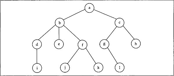
The tree on the previous page has twelve nodes with root node as a at the top, and having no incoming arcs. The nodes such as i, e, j, k, 1, h do not have any outgoing arc and are called leaves. The nodes that are directly accessible from a given node are called children of that node. A node is a parent of its children. For example, d, e, f are the children of b, while b is the parent of d, e and f. The nodes d, e, f have the common parent b and so they are siblings. If there is a path from node n1 to node n2 we say n1 is an ancestor of n2 and n2 is a descendant of n1. For example, c is an ancestor of 1 and 1 is a descendant of c. Clearly, a node is an ancestor and descendant of itself. An ancestor or descendant, which is different from itself, is known as a proper ancestor or proper descendant, respectively. So the other way of defining a leaf is a node with no proper descendant.
The depth or level of a node may be defined as follows: the depth of the root node is 0 and the depth of any other node in the tree is the depth of its parent plus 1, that is, depth of a node is actually the length of the unique path from root to that node. The height of a tree is the depth of the node that is at the largest depth in the tree plus 1.
In the following sections we will discuss a more specific type of tree: the binary tree. This type of tree has many applications and has different forms. In a binary tree there are at the most two outgoing arcs from a node. If every intermediate (non-leaf) node in a binary tree has exactly two non-empty children, then it is a strictly binary tree. In case in a strictly binary tree all the leaves are at a same depth d say, it becomes a complete binary tree. The binary tree in Fig. 12.1 is a complete binary tree of depth 3 and hence also a strict binary tree.
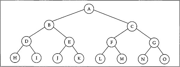
Fig. 12.1 A complete binary tree of depth 3
Clearly, in a binary tree if there are b nodes at depth d then at depth (d+1) there is a maximum of 2b nodes. So in a complete binary tree of depth d there are 2d leaf nodes. Hence the total number of nodes in a complete binary tree of depth d is given by t where
t = 1 + 21 + 22 +…+ 2d
= 2(d+1)–1
12.2 BINARY TREES
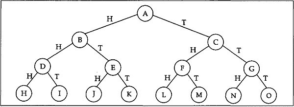
Fig. 12.2 Each path marked in a binary tree
Trees in which every node has a maximum of two children are called binary trees. For example, a binary tree is shown in Fig. 12.2. Each path from the root to a leaf node of this tree corresponds to a particular outcome in flipping a coin three times in succession. For instance, the path A-C-F-L represents the outcome THH in the diagram.
A formal recursive definition of a binary tree may be written as follows:
A binary tree is either empty, that is, it is a binary tree with no nodes, or consists of a node called the ‘root’ which has two pointers to two different binary trees called ‘left subtree’ and ‘right subtree’.
Note that left subtree and right subtree are two different binary trees and hence we distinguish between them, that is, the binary trees shown in Fig. 12.3 are two distinct binary trees in the sense that the root of the binary tree in Fig. 12.3(a) has an empty right subtree while the root of the binary tree in Fig. 12.3(b) has an empty left subtree. It is also to be noted that a binary tree having n nodes has (n-1) arcs (edges).
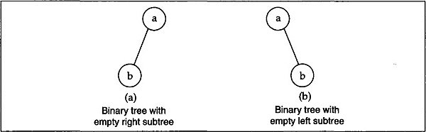
Fig. 12.3
The above definition suggests a natural implementation of binary tree using linked structure. Each node in the binary tree has two links, one pointing to the left subtree of the node (this link will be NULL if the left subtree is empty) and the other pointing to its right subtree (NULL if empty right subtree), together with an information part. Since each node of the binary tree can be reached from the root by following a unique path from the root, a pointer to the root of the binary tree will allow us to access any node of the binary tree. So we make the following declarations to implement a binary tree:
typedef struct treetype{
            int   info;             /* Information part */
            struct treetype *left;  /* Pointer to left subtree */
            struct treetype *right; /* Pointer to right subtree */
            } treenode;
typedef treenode *nodeptr;
nodeptr tree; /* Pointer to the root of the binary tree */
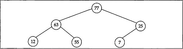
In the above declaration we assumed the information part of each node in the binary tree as an integer value. Instead of using int as the typename of the information part one should replace the suitable typename that fits the actual problem domain. For illustration, consider the following binary tree with integers as the information part of each node.
The linked representation of the binary tree will look like the following:
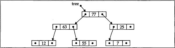
In the above picture the pointer that is not linked to a node is a NULL pointer. This style is followed throughout the chapter.
12.3 TRAVERSALS OF BINARY TREE
Binary trees are used to organize data so that they can be accessed very efficiently in many applications. Most of such applications need to be able to walk through all the nodes of the binary tree by visiting it exactly once. This walking through the tree is referred to as the process of traversing the binary tree. Clearly, a linear order of nodes is the outcome of a complete traversal of a binary tree and this linear order depends on the traversal algorithm. The definition of binary tree suggests that a traversal algorithm requires the following three basic steps:
(a) visit a node (denoted in this book as T),
(b) traverse the left subtree (denoted as L), and
(c) traverse the right subtree (denoted as R).
Obviously, the orders in which these steps are performed determine the order of the node visited in the tree. Moreover, there are 3! different orders in which these steps can be performed. These are given by
LTR
TLR
LRT
RTL
RLT
TRL
The ordering LTR corresponds to the following traversal algorithm:
if (the binary tree is non-empty)
{
       traverse left subtree;
       visit the root;
       traverse right subtree;
}
It can easily be understood that the last three orders are very much similar to the first three orders in the above list. The first three orders are the principal orders of traversal and named as follows:
LTR — inorder traversal
TLR — preorder traversal
LRT — postorder traversal
It is simple to implement either of these algorithms by writing a recursive function. Before writing the functions we assume the existence of a function visit (treenode *node) which performs the desired task (visit) for the node pointed by the pointer node. For our purpose let us consider the function visit as in the following, which prints the information part of the node visited.
void visit(treenode *node)
{
      printf (“%d	”, node->info);
}
We also assume that the pointer tree points to the root of the tree. The three traversal functions inorder, preorder, and postorder are listed below in examples 12.1, 12.2 and 12.3 respectively.
Example 12.1
 /* Inorder traversal function*/
 void inorder(treenode *tree)
 {
      if (tree)
      {
           inorder (tree->left);
           visit (tree);
           inorder (tree->right);
      }
 }
Example 12.2
 /* Preorder traversal function */
 void preorder(treenode *tree)
 {
      if (tree)
      {
           visit (tree);
           preorder (tree->left);
           preorder (tree->right);
      }
 }
Example 12.3
 /* Postorder traversal function */
 void postorder(treenode *tree)
 {
      if (tree)
      {
           postorder (tree->left);
           postorder (tree->right);
           visit (tree);
      }
 }
To visualize that the names preorder, inorder, and postorder are appropriate, consider the following arithmetic expression A*B+C/D-E. Notice that this is an infix expression and uses only binary operators (+, -, *, /). A binary tree may be used to represent this expression. The binary tree that represents an expression is known as an expression tree. The expression tree for the above expression is shown in Fig. 12.4.
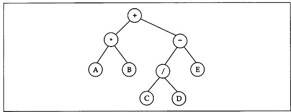
Fig. 12.4 Expression tree for the infix expression A * B + C/D - E
From Fig. 12.4 it can be seen that all the operands of the expression appear at the leaf of the binary tree. Moreover, the preorder traversal of this tree gives the expression
+ *AB -*CDE
which is the prefix expression. The inorder traversal generates the original infix expression A*B + C/D - E. It can also be seen that the postorder traversal of the tree generates the postfix(RPN) expression AB*CD/E -+.
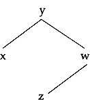
At this point we should be little careful to notice that different binary trees may have the same traversal sequence. For example, the inorder traversals of the tree in Fig. 12.5(a) and Fig. 12.5(b) have the same sequence x y z w. It is clearly seen that though the inorder traversal sequences of these two trees are the same, their preorder traversals y x w z and w z y x are not the same. In fact, there is only one binary tree corresponding to a given inorder and preorder sequence. The construction of such a binary tree is also interesting. Let us construct a binary tree for which the inorder traversal sequence is given as x y z w and the preorder sequence as y x w z.

Fig.12.5 Same inorder sequence of two different trees
From the preorder sequence it is clear that the root of the binary tree contains y and it is of the form as shown on the next page, where T1 and T2 are the left and right subtree, respectively.
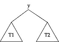
From the above tree it can be said that the inorder sequence of this is of the following form: (inorder sequence of T1 subtree) y (inorder sequence of T2 subtree).
This form, when matching with the given inorder sequence, tells us that the inorder sequence of T1 subtree is x and the inorder sequence of T2 subtree is z w. This, in turn, concludes that T1 is a single node subtree containing x, but T2 is having more than one node. Clearly again from the given preorder sequence we can conclude that T2 subtree has a preorder sequence w z since T1 is a single node subtree containing x. Thus the subtree T2 may be drawn as below which is having its root containing w with a left subtree T3 and a right subtree T4. Obviously its inorder traversal is of the form
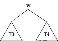
(inorder sequence of T3 subtree) w (inorder sequence of T4 subtree) and is given by z w. Hence the inorder sequence of T3 is z and the inorder sequence of T4 is NULL. So the required binary tree will look like
12.4 THREADED BINARY TREE
Binary tree traversals are important operations in many applications. For an inorder traversal, we have seen, one has to recursively traverse the left subtree first, then visit the root, and finally traverse the right subtree. Clearly, because of the recursive nature of the routine an implicit stack is maintained which allows to backtrack whenever necessary. So, for backtracking purpose an explicit stack must be maintained by a routine that implements inorder traversal non-recursively. Threaded binary tree is nothing but a simple modification to the ordinary binary-tree structure. This modification allows inorder traversal of a binary tree without any recursion that uses no stack.
In a binary tree the inorder successor of a node M is the node N that appears immediately after the node M in the inorder traversal of the binary tree. In recursive algorithms this inorder successor can easily be found by automatic backtracking. As we mentioned earlier, to do this backtracking a non-recursive algorithm must maintain an explicit stack. A careful look at the binary tree tells that if the right subtree of a node is non-empty then its inorder successor must be found in this right subtree, otherwise we need to do backtracking to find it out. In this case, since the right subtree of the node is NULL, that is, the right link of the node is NULL, a threaded tree uses this link to keep the pointer that points to its inorder successor. Here we must be careful that this link should not be confused with the link to its right subtree (because actually there is no such right subtree for the node). This link is known as a thread. To identify that this is just a thread and not a link to its right subtree, an extra logical field is added to each of the tree nodes and may pictorially be shown as in Fig. 12.6.
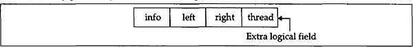
Fig. 12.6 Node structure of a threaded binary tree
Thus a node in threaded binary tree may be defined as follows:
typedef struct treetype{
            int info;
            struct treetype   *left;
            struct treetype   *right;
            int thread; /* thread=l implies right link is a thread
                            and is not pointing to right subtree */
            } treenode;
typedef treenode *nodeptr;
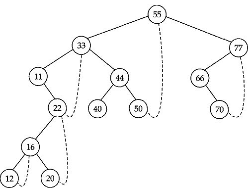
For illustration, consider the following binary tree.
The binary tree with threads equivalent to this binary tree is shown below.
A function to implement the inorder traversal in a threaded binary tree may be written as in example 12.4:
Example 12.4
 thread_in(nodeptr treeptr)
 {
      nodeptr    ptrl, ptr2;


      ptr1 = treeptr;
      do    {
            ptr2 = NULL;
            while (ptr1 != NULL)
            {
               ptr2 = ptr1;
               ptr1 = ptr1->left; .
            }
            if (ptr2 != NULL) /* Non Null treeptr */
            {
                  printf(“%d
”, ptr2->info); /* Visit node */
                  ptr1 = ptr2->right;
                  while (ptr1 != NULL && ptr2->thread)
                  {   /* Visit inorder successor through thread */
                     printf(“%d
”, ptr1->info);
                     ptr2 = ptr1;
                     ptr1 = ptr1->right;
                  }
             }
       } while (ptr2 != NULL);
 }
12.5 BINARY SEARCH TREES
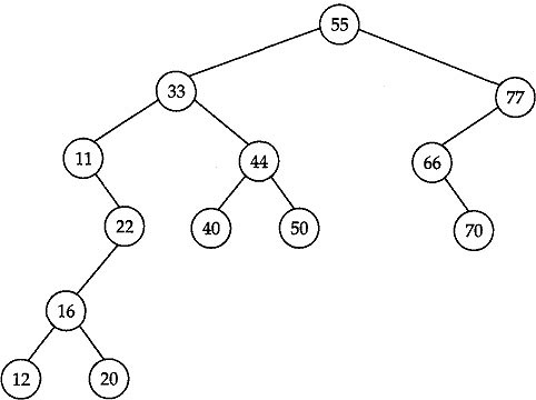
Binary search tree (BST) is an important data structure which is a special type of binary tree (having specific properties) used mainly in applications where tree sorting and searching is necessary. To illustrate the properties of a binary search tree consider the binary tree shown in Fig. 12.7. This binary tree has nodes that correspond to the records whose keys are alphabetic names (some of the characters from the Mahabharata) given by (in alphabetical order) Arjuna, Bhima, Bidur, Draupadi, Duryodhana, Ganga, Judhistra, Kama, Krishna, Nakul, Sahadeva, Sakuni and Viswa.
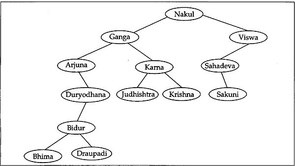
Fig. 12.7 A Binary Search Tree
Though the binary tree in Fig. 12.7 is little awkward, it has the property that the value(name) in every node in this tree is such that the root node of its left subtree holds a value which is either NULL or less than (in lexicographic order) the node and the root node of its right subtree holds a value which is either NULL or greater than (in lexicographic order) the node. Because of this property it can be seen that if we traverse this binary tree using inorder traversal we visit the nodes in the order Arjuna, Bhima, Bidur, Draupadi, Duryodhana, Ganga, Judhistra, Kama, Krishna:, Nakul, Sahadeva, Sakuni and Viswa, which is nothing but the alphabetic order.
A careful look at Fig. 12.7 concludes the following observations to this binary tree.
- Each different node has a distinct value(name), that is, no two nodes in this binary tree have the same value.
- The value of every node in this binary tree is greater than (in lexicographic order) the value in its left child (if it exists).
- The value of every node is less than the value in its right child (if it exists).
A binary tree having this property is called a binary search tree (BST). Once the information is organized in a BST, the search process becomes simpler. For example, if we want to search whether the name Judhistra is there in the list one may traverse the tree in the following manner.
Begin the search by traversing the root of the tree.
Is it Judhistra?
Response is no. (It is Nakul)
Is it less than Judhistra?
Response is no. (Means it is greater than Judhistra)
Traverse the left subtree by traversing its root.
Is it Judhistra?
Response is no. (It is Ganga)
Is it less than Judhistra?
Response is yes.
Traverse the right subtree by traversing its root.
Is it Judhistra?
Response is no. (It is Kama)
Is it less than Judhistra?
Response is no. (Means it is greater than Judhistra)
Traverse the left subtree by traversing its root.
Is it Judhistra?
Response is yes.
Obviously, if we try to search for the name Jayadhrata in this BST, the response of the last comparison will be ‘no’ and as the name Jayadhrata is less than Judhistra in lexicographic order, the left subtree of Judhistra is to be searched. Since the left subtree is NULL, we conclude that Jayadhrata is not present in the BST. In this case since the check that the left subtree is NULL, we see that one more comparison is necessary. A BST may be implemented as follows:
 typedef struct treetype{
                        char info[15]; /* Node information type */
                        struct    treetype    *left;
                        struct    treetype    *right;
                        }    treenode;
 typedef    treenode    *bst_ptr;
 bst_ptr    rootptr;    /* Pointer to the root of the BST */
A function to search a key in a binary search tree may now be implemented as in the following example 12.5. The function bst_search ( ) is searching for a node with specified key in a BST. It accepts two arguments:
(i) the pointer rootptr to the root of the BST, and
(ii) an item indicating the node information key
If the search is successful, the function returns a pointer to the node containing the specified item. If not successful, it returns a NULL pointer. The function that follows is a recursive function. Its main drawback is that in some situations it may require a very large stack space.
Example 12.5
 bst_ptr bst_search(bst_ptr   rootptr, char   item[])
 {

      bst_ptr   curptr; /* Current search pointer */
      int 1 ;
      if (rootptr != NULL)   /* If the BST is non-empty */
      {
           curptr = rootptr;
           if ( (l=strcmp(item, curptr->info)) < 0 )
                 /* Search left subtree */
                 curptr = bst_search(curptr->left, item);
           else if (1 > 0)
                 /* Search right subtree */
                 curptr = bst_search(curptr->right, item);
           else
                 return curptr;
      }
      return NULL;
 }
12.5.1 Building a Binary Search Tree
Let us now concentrate on the process of creating a BST from scratch. For illustration we consider the data set from which the BST will be created as the set of names used earlier stored in an initialized array of pointers given below.
char   *a[] = {
              “Arjuna”,
              “Bhima”,
              “Bidur”,
              “Draupadi”,
              “Duryodhana”,
              “Ganga”,
              “Judhistra”,
              “Karna”,
              “Krishna”,
              “Nakul”,
              “Sahadeva”,
              “Sakuni”,
              “Viswa”
              } ;
We write a function build_bst ( ) to build a BST from this array(data-set). The function should receive the following arguments: pointer to pointer to the root node of BST, possibly a NULL pointer at the beginning; a pointer to array containing the data set, and finally the array size, that is, the number of elements in the data set.
The function build_bst ( ) may be implemented as in the following.
 build_bst (bst_ptr   *rootptr, char   *data[], int   size)
 {
      int index;
      for (index=0; index<size; index++)
           insert_bst(rootptr, data[index]);
      return;
 }
Basically, the above function simply loops through the elements to insert that element in the BST using the function insert_bst ( ). Clearly, as this insert_bst ( ) function actually allows to insert an element into a BST, it must receive the following arguments: pointer to pointer to the current subtree node (the root of the current subtree) under which the element is to be inserted; and the element to be inserted. In our case, as it is a string of characters (a name), this argument is a pointer to the string.
The function insert_bst (bst_ptr *rootptr, char *element) first checks if *rootptr is NULL to identify whether the BST is empty or not. If so, then insert the element as the root of the BST and accordingly set the new value of *rootptr. If the original BST is not empty then compare the element with root (that is, the root of each subtree) and move to the left or right subtree depending on whether the element is smaller or larger than the root of each subtree. In case the element matches with the root, that is, there is a node with the same element, it simply returns from the function. Our implementation is a recursive one, though in some cases it may require a large stack. The function insert_bst ( ) is listed in example 12.6.
Example 12.6
 insert_bst(bst_ptr *rootptr, char *element)
 {    /* A recursive version */
      bst_ptr newptr;
      int c;
      if (*rootptr == NULL)
      {
           newptr = (bst_ptr) malloc(sizeof(treenode));
           newptr->left = NULL;
           newptr->right = NULL;
           strcpy(newptr->info, element);
           *rootptr = newptr;
      }
      else
      {
           if ((c=strcmp(element, (*rootptr)->info)) == 0)
                return;    /* Element already present in the BST */
           else if (c<0)    /* Insert element to the left subtree */
                insert_bst( &(*rootptr)->left, element );
           else         /* Insert element to the right subtree */
                insert_bst( &(*rootptr)->right, element );
      }
 }
With respect to time an iterative component of this function is more advantageous. An iterative function insert_bst_iter ( ) that searches a binary search tree and inserts a new element into the tree if the search is unsuccessful may be implemented as shown in example 12.7. This time let the arguments to the function be the following.
(i) A pointer to the root of the BST, instead of a pointer to pointer to the root as in the case of recursive version given earlier.
(ii) The element to be inserted.
The function returns a pointer to the inserted node if successful, otherwise returns the pointer to the node where the element is already present. It may be written as follows:
Example 12.7
 bst_ptr    insert_bst_iter(bst_ptr    rootptr, char *element)
 {
      bst_ptr    ptr1, ptr2, newptr;
      int c;


      ptr1 = rootptr;
      ptr2 = NULL;
      while (ptr1 != NULL)
      {
           if ((c=strcmp(element, ptr1->info)) == 0)
                /* Element already present in the BST */
                return ptr1;
           ptr2 = ptr1;
           ptr1 = (c < 0)? ptrl->left: ptrl->right;
      }
      newptr = (bst_ptr)malloc(sizeof(treenode));
      newptr->left = newptr->right = NULL;
      strcpy(newptr->info, element);
      if (ptr2 == NULL)
           rootptr = newptr;
      else if ((c=strcmp(element, ptr2->info)) < 0)
           ptr2->left = newptr;
      else
           ptr2->right = newptr;
      return newptr;
 }
It may easily be noted that after insertion of a node into a BST using the above routine the resulting tree still remains to be a BST.
12.5.2 Deleting a Node from a Binary Search Tree
Deletion of a node from a BST is more complex than insertion. We need to consider three cases to delete a node from a BST. These are as follows:
(i) The node to delete is a leaf.
(ii) The node to delete has only one non-empty child (either left or right).
(iii) The node to delete has two non-empty children.
The first case is very simple. Since the node to delete has no child, it may simply be deleted by setting the appropriate (left or right) pointer in its parent node to NULL, and freeing the node itself.
For example, to delete the leaf node containing 111 from the BST in Fig. 12.8 we simply set the right pointer in its parent containing 99 to NULL and free the node 111. The BST after deletion looks like in Fig. 12.9.
The second case is also very simple. For example, if we want to delete the node containing 35 (having one non-empty child), from the BST in Fig. 12.9, we need to set the right pointer in the node containing 25 (that is, the appropriate pointer of the parent node of the node to delete) to the node containing 39 (that is, the only child of the node to delete). After deleting the node with 35 the BST takes the form as shown in Fig. 12.10.
These two cases discussed above can be combined together to a function where the node to be deleted has at the most one subtree. It can easily be understood that such a function requires (i) the pointer to the node to delete (say delptr), and (ii) the pointer to the parent of the node to delete (say pptr).
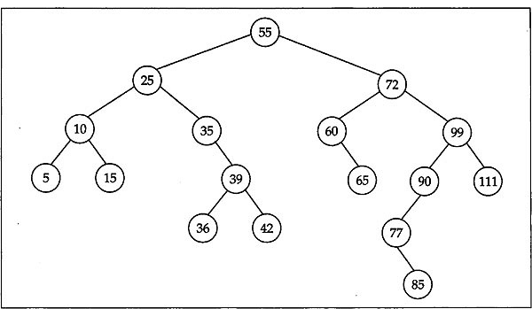
Fig. 12.8 BST of integers from which the leaf 111 is to be deleted
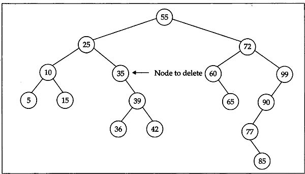
Fig. 12.9 BST configuration after deletion of 111 from Fig. 12.8
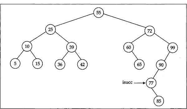
Fig. 12.10 BST configuration after deleting 35 from BST in Fig. 12.9
So, to delete a node from a BST for a given information part, we must first search the BST to get the above two pointers and then only we can delete the node from the BST. Our algorithm uses the following variables whose purpose are listed.
delptr: pointer to the node to delete
pptr: pointer of the parent of the node to delete.
auxptr: an auxiliary pointer that will be set to the pointer to the node by which delptr will be replaced.
The following function in example 12.8 deletes the node for which the information part is given by val(an integer value) say, from the BST whose root is pointed by the argument tree. If such a node is not found, no node is deleted and simply returns leaving the BST unaltered. If the node is found in the BST, the function deletes the node from it and returns the pointer to the root of the modified BST (after deleting the node) which is also a BST.
Example 12.8
 bst_ptr bst_delete(bst_ptr tree, int val)
 /* tree is the pointer to root of the BST *7
 /* val is the information part of the node to delete */
 {
      bst_ptr    delptr, pptr;
      bst_ptr    auxptr;      /* An auxiliary pointer */
      /* Initialize */
      delptr = tree;
      pptr = NULL;
      /* Find node with value val(if any). If found set delptr to
      point to the node and pptr to point to its parent(if exists) */
      while (delptr != NULL && delptr->info != val)
      {
           pptr = delptr;
           delptr = (val < delptr->info)? delptr->left: delptr->right;
      }
      if (delptr == NULL)   /* Val not found */
           return tree;
      /* We assume delptr has at the most one child */
      /* Set auxptr to point to the node by which the node pointed by
         delptr will be replaced */
      auxptr = (delptr->left == NULL)? delptr->right: delptr->left;
      if (pptr == NULL) /* Node to be deleted is the root itself */
      tree = auxptr;
      else
      (delptr ==pptr->left)? pptr->left = auxptr: pptr->right = auxptr;
      free(delptr);
      return tree;
 }
The functionbst_delete ( ) given above considers only the first two cases of deleting a node from a BST. The last case where the node to be deleted having two non-empty children is yet to be considered. This case can also simply be reduced to one of the first two cases. This can be achieved by replacing the node to be deleted by its inorder successor (or predecessor) and deleting this inorder successor (or predecessor) from the BST. The inorder successor (or predecessor) of the value stored in a given node is the successor (or predecessor) of the node in the inorder traversal of the tree. For illustration, consider the tree in Fig. 12.10 where we want to delete the node in which the stored value is 72. Clearly, this node is having two nonempty children. Now we need to locate the inorder successor of this node. A careful look at inorder traversal process claims that we can reach the inorder successor of a node by starting at its right child and then descending through the left child as far as we can. In our case this node is the node with value 77, and is pointed by isucc in Fig. 12.10. To delete the node with value 72, we first replace the content of this node by the content of its inorder successor node (that is, the node with value 77). Then we need only to delete this inorder successor. Obviously, this successor node will always have an empty left subtree. So this deletion can simply be done by one of the first two cases. After replacing the node with value 72 by the value of its inorder successor node the tree will look as in Fig. 12.11.
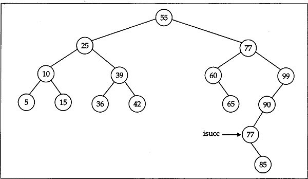
Fig. 12.11 BST configuration after replacement by inorder successor
Finally, after deleting this inorder successor the tree takes the form depicted in Fig. 12.12.
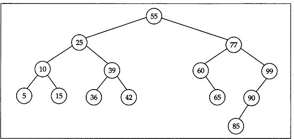
Fig. 12.12 BST configuration after deleting inorder successor
Combining this case with the function bst_delete ( ) we wrote earlier, the function is finally written as in example 12.9.
Example 12.9
 bst_ptr    bst_delete(bst_ptr    tree, int val)
 /* Tree is the pointer to the root of the BST */
 /* Val is the information part of the node to delete */
 {
      bst_ptr      delptr, pptr, auxptr;
      bst_ptr      pauxptr, 1ptr;

      delptr = tree;
      pptr = NULL;
      /* Find node with value val(if any). If found, set delptr to
      point to the node and pptr to point to its parent node */
      while ( delptr!=NULL && delptr->info!=val)
      {
           pptr = delptr;
           delptr = (val<delptr->info)? delptr->left: delptr->right;
      }
      if (delptr == NULL)      /* Val not found */
             return tree;      /* Tree unchanged */
      /* Set auxptr to point to the node by which the node delptr
      will be replaced */
      if (delptr->left == NULL)
           auxptr = delptr->right;
      else if (delptr->right == NULL)
           auxptr = delptr->left;
      else { /* delptr has two nonempty children */
             /* Set auxptr to the inorder successor of delptr and
                pauxptr to the parent of auxptr */
           pauxptr = delptr;
           auxptr = delptr->right;
           lptr = auxptr->left;
           while (lptr != NULL)
           {
                pauxptr = auxptr;
                auxptr = 1ptr;
                lptr = auxptr->left;
           }
           /* auxptr is now pointing to inorder successor of delptr */
           if (pauxptr != delptr)
           { /* delptr is not parent of auxptr and so auxptr->left
           equals pauxptr */
                pauxptr->left = auxptr->right;
                auxptr->right = delptr->right;
           }
           auxptr->left = delptr->left;
      }
      if (pptr == NULL)
           tree = auxptr;
      else
      (pptr->left==delptr)? pptr->left=auxptr:pptr->right = auxptr;
      free(delptr);
      return tree;
 }
12.6 AVL TREES
In the earlier sections we have discussed binary trees, threaded binary trees, and binary search trees. From the above discussions it is easy to understand that in case of a BST the search time is O(log n) in the best case but in the worst case (where the BST is degenerated) the search time is O(n). This suggests that if the tree is uniform in nature the search time for a node will be reduced. The performance of an algorithm using trees mostly depends on how quickly we can search for a node in the tree and so the reduction in search time of a node in a tree is of great importance.
An AVL tree is basically a BST in which the heights of the two subtrees of each node in the tree never differ by more than one. That is why it is also called as height balanced tree. The name AVL tree is after the two Russian mathematicians, G M Adelson-Velskii and E M Landis, who discovered this sort of trees in 1962.
It is easy to visualize that the height of an ordinary binary tree can be O(n) where n is the number of nodes in the tree and is degenerated to one side. Hence the search time for a node in such type of tree is also O(n). Obviously, as n increases, the performance degrades. In case of AVL trees, the maximum number of nodes n is given by n = 2h –1, where h is the height of the tree. So h = log2 (n+1)=O(log2 n). Hence the time to search for a node traversing the full height of an AVL tree having n nodes from the root to a leaf node is O(log2 n) and is significantly less than O(n).
An AVL (height balanced) tree must keep information about the balance between the heights of the left and right subtrees of each node in the tree. The balance of a node is defined as the difference between height of its left subtree and the height of its right subtree, that is,
balance = height of left subtree – height of right subtree
The operations on a BST and an AVL tree are very much similar except for insertion of a node into an AVL tree and deletion of a node from an AVL tree. After insertion and deletion of nodes into and from an AVL tree the balance is maintained. The above discussion suggests the implementation of an AVL tree as follows.
 typedef   int   data_type;
 typedef   struct       avl {
                        data_type info;
                        struct    avl    *left;
                        struct    avl    *right;
                        int       balance;
                       }    avlnode;
 typedef avlnode *avlptr;
12.6.1 Inserting a Node into an AVL Tree
Obviously, the insertion of a node into a NULL tree(AVL) is trivial. In case where the AVL tree is not NULL we need to determine the search path, the path from the root node to the node where the insertion should take place. Clearly, if the node to be inserted is already found in the AVL tree, the insertion is skipped. Otherwise, the node is inserted to the AVL tree just as we did in case of binary search tree in Section 12.5. After inserting the node into the AVL tree, the tree may not remain height balanced. If it becomes imbalanced, as part of insertion, this unbalanced tree is then rebalanced to ensure the height balance of the AVL tree.
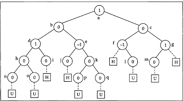
Fig. 12.13 Different situations of unbalancing in an AVL tree
At this point we must first determine what are the situations where an insertion of a node makes an AVL tree unbalanced. To visualize this let us consider a tree in Fig. 12.13. The figure indicates different insertion points by using dashed lines into an AVL tree. Each node in the tree in the above figure is named with an alphabet. Each node of the AVL tree holds the balance value within it before any insertion. At each insertion point a square box is connected with a dashed line. The value H within a square box indicates that if an insertion takes place at the corresponding point the AVL tree will remain height balanced and the value U indicates that because of insertion the tree will be unbalanced. A careful look at Fig. 12.13 claims that the tree becomes unbalanced only in two situations.
These situations are given in the following.
- When the newly inserted node is a left descendant of a node that previously had a balance of 1.
- When the newly inserted node is a right descendant of a node that previously had a balance of –1.
In Fig. 12.13 the unbalance of the tree for insertion of a node at nodes n, o, and m is due to the reason mentioned in the first case, and the same at nodes p, q, and 1 is due to the second case. The youngest ancestor that becomes unbalanced at each insertion is listed below.
- d becomes unbalanced for insertion at n and o.
- e becomes imbalanced for insertion at p and q.
- f becomes unbalanced for insertion at 1.
- g becomes unbalanced for insertion at m.
So from now we will concentrate on the subtree that is rooted at the youngest ancestor and becomes unbalanced as a result of insertion of a node. Firstly, consider the balance of this youngest ancestor as 1. Let the youngest ancestor that has become unbalanced be P and the root of its left subtree be Q. Clearly Q is non-null since P has a balance of 1. It should also be noted that since P, the youngest ancestor of the new node, has become unbalanced the node Q must be of balance 0 before insertion, that is, both the left and right subtrees of Q are of the same height n (say). Clearly in that case, the height of the right subtree of P should also be n because of height balance property. In fact, these subtrees of height n may also be NULL, that is, the value of n may also be 0. A careful analysis claims that P becomes unbalanced in only two situations illustrated in Fig. 12.14. In Fig. 12.14(a) the new node is inserted into the left subtree of Q so that it changes the balance of Q to 1 and balance of P to 2. In the other case the new node is inserted into the right subtree of Q so that it changes the balance of Q to –1 and balance of P to 2 which is shown in Fig. 12.14(b).
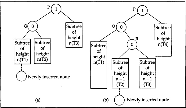
Fig. 12.14 Unbalancing situations
These unbalanced trees must now be rebalanced to maintain the height balance property. At this point we must also ensure that after rebalancing the inorder traversal of the tree and the same for the previous unbalanced tree must match. Before rebalancing, let us shift our concentration a little for the time being. We will come back into our main discussion shortly.
Consider the tree rooted at a shown in Fig. 12.15(a). If we apply a left rotation to this rooted tree at a we will get the tree as shown in Fig. 12.15(b). Notice that the root of this new tree is changed to c but the inorder sequences of both the trees are the same. An algorithm to implement this left rotation to a tree rooted at x (pointer to the root of the subtree) may simply be written as in the following.
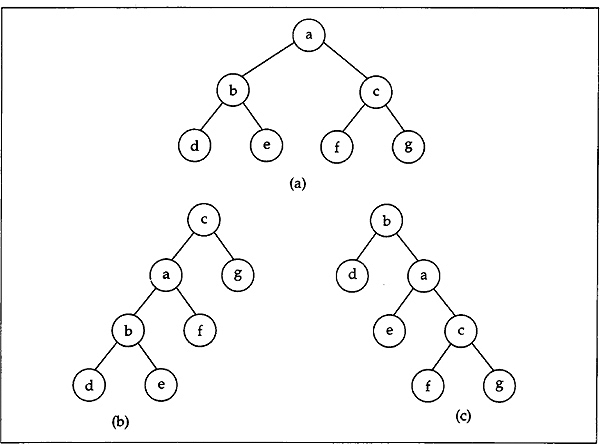
Fig. 12.15 Left and right rotation of rooted trees
y = x->right;
save = y->left;
y->left = x;
x->right = save;
For illustration, the right rotation of the rooted tree in Fig. 12.15(a) is shown in Fig. 12.15(c). Here the root of the rotated tree is changed to b. But again the inorder sequence of this rotated tree is same as that of the tree in Fig. 12.15(a).The algorithm to implement the right rotation to a tree rooted at x may be written as in the following.
y = x->left;
save = y->right;
y->right = x;
x->left = save;
We have seen that both left and right rotations of trees are preserving the inorder sequence. So to rebalance an unbalanced tree we may apply any number of left or right rotations to the imbalanced tree which will also preserve the inorder sequence.
Now let us turn our concentration to the main discussion. To maintain the height balance property of the tree in Fig. 12.14(a) we simply apply a right rotation on the subtree rooted at P. This right rotation will yield a new subtree rooted at Q shown in Fig. 12.16. The figure also shows the balance value of the nodes after rotation.
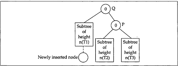
Fig. 12.16 Tree after right rotation of three in Fig. 12.14(a)
The unbalanced subtree in Fig. 12.14(b) requires a little more attention. Here the new node is inserted into the right subtree of Q. Let R be the root of the right subtree of Q. Apparently, there are three different situations for insertion. But they are analogous to each other. These three situations are
- R itself may be the newly inserted node (arises when n=0).
- New node is inserted into the left subtree of R.
- New node is inserted into the right subtree of R.
We discuss the situation in Fig. 12.14(b) that illustrates the case where the new node is inserted into the left subtree of R. At first we give a left rotation to the subtree rooted at Q. After this rotation the subtree rooted at P will look like in Fig. 12.17(a).
Note that after this rotation the inorder sequences of the subtrees in Fig. 12.14(b) and Fig. 12.17(a) are same. To rebalance, finally we give a right rotation to the subtree rooted at P shown in Fig. 12.17(a). After this right rotation the final subtree will look like in Fig. 12.17(b). Here also it should be noted that the inorder sequence of this subtree and that of the subtree in Fig. 12.14(b) are the same. The other case is very much similar (symmetrical) to the above and is left to the reader. A C function avl_insert ( ) is presented below. The function allows to search and insert an element into an AVL tree. The implementation of a node in AVL tree is discussed earlier in this section. The function shown in example 12.10 returns the pointer to the root of the AVL tree after node insertion.

Fig. 12.17 Rebalancing the tree in Fig. 12.14(b)
Example 12.10
 avlptr avl_insert(avlptr tree, data_type item)
 {
      int imbal_dir; /* Imbalance direction */
      avlptr p = tree,
             y = p, /*y points to the youngest unbalanced ancestor*/
            cy = NULL, /* cy points to the child of y */
            py = NULL, /* py points to the parent of y */
            pp = NULL, /* pp points to the parent of p */
             q = NULL; /* q points to the new node */

      /* Search into the AVL tree(also a BST) */
      while ( p != NULL )
      {
            if ( p->info == item )
                  return(p);
            q = ( item < p->info )? p->left: p->right;
            if ( q != NULL && q->balance != 0 )
            {
                  py = p;
                  y = q;
            }
            pp = p;
            p = q;
      }
      /* Insert new record into the BST */
      q = (avlptr)malloc( sizeof(avlnode) );
      q->info = item;
      q->left = q->right = NULL;
      q->balance = 0;
      (item < pp->info)? pp->left = q: pp->right = q;
      /* At this point the balance between q and y must be adjusted because of insertion */
      p = (item < y->info)? y->left: y->right;
      cy = p;
      while ( p != q )
            if (item < p->info)
            {
                  p->balance = 1;
                  p = p->left;
            }
            else {
                  p->balance = -1;
                  p = p->right;
            }
      /* Check if the tree has become unbalanced */
      imbal_dir = (item < y->info)?1 : -1;
      if (y->balance == 0)
      { /* Another level is added to the tree and since y is the youngest ancestor, the tree remains balanced */
      y->balance = imbal_dir;
      return(q);
 }
 if (y->balance != imbal_dir)
 {     /* Node is inserted to the opposite direction of imbalance, so the tree remains balanced */
       y->balance = 0;
       return(q);
 }
 /* Now it has been found that the tree has become unbalanced.
    Rebalance the tree by applying required rotations and adjusting
    the balance of involved nodes */
 /* Note that, q is pointing to the inserted node,
             y is pointing to its youngest unbalanced ancestor,
             py is pointing to the parent of y,
     and     cy is pointing to the child of y in the direction of imbalance */
 if ( cy->balance == imbal_dir )
 {     /* cy and y are unbalanced in same direction */
      P = cy;
      (imbal_dir == 1)? rotate_right(y): rotate_left(y);
      y->balance = 0;
      cy->balance = 0;
 }
 else { /* cy and y are unbalanced in opposite directions */
      if (imbal_dir == 1)
      {
             p = cy->right;
             rotate_left(cy);
             y->left = p;
             rotate_right(y);
      }
      else {
             p = cy->left;
             rotate_right(cy);
             y->right = p;
             rotate_left(y);
      }
      /* Now adjust balance of nodes involved */
      if (p->balance = 0)
      {     /* p is the node inserted */
             y->balance = 0;
             cy->balance = 0;
      }
      else if (p->balance == imbal_dir)
      {
             y->balance = -imbal_dir;
             cy->balance = 0;
      }
      else   {
             y->balance = 0;
             cy->balance = imbal_dir;
      }
      p->balance = 0;
      }
      if (py == NULL)
             tree = p;
      else if (y == py->right)
             py->right = p;
      else
             py->left = p;
      return(q);
 }
12.6.2 Deleting a Node from an AVL Tree
In case the AVL tree consists of a single node the deletion is simple. Otherwise we first delete a node containing x (say) from an AVL tree (having more than one node) just as we did in case of a BST. Then we rebalance the tree to maintain the height balance property of the AVL tree.
Consider that the deletion of the node has occurred at the node point by p. Then obviously the height of the subtree rooted at p has reduced by one. Let pp be the parent of the node p. Check the balance of pp. We may now rebalance the subtree rooted at pp as we did in insert, if required. If we find that the height of the subtree rooted at pp is not reduced then deletion from AVL tree is over. Otherwise, we move one step up towards the root and do the same. In fact, in the worst case we may have to look at the root. The complexity of deletion is more than that of insertion (though the same concept of rotations is used) because in case of deletion we may need as much rebalancing as the path length from the deleted node to the root. The C implementation of this deletion process is left as an exercise to the reader.
12.7 B-TREES
B-trees are basically the general form of BSTs in which a node can have more than one information part. These are balanced search trees which are very much useful for external searching and work well in secondary storage devices. Consider a node that can have a maximum of m children in the tree. We say that it is a B-tree of order m. In a B-tree all leaf nodes are at the same level. If a node is having exactly k non-empty children, then the node contains exactly (k-l) keys. The leaf nodes and the intermediate nodes are distinguishable. Precisely speaking, a B-tree of order m is maintaining the following properties.
- Each internal node except possibly the root has at the most m non-empty children and at least [m/2] non-empty children. The root may have no children or any number of children between 2 to m.
- Each internal node may have at the most (m-1) keys and the node will have one more child than the number of keys it has.
- Within a node all the keys are arranged in a predefined order. All keys in the subtree to the left of a key are predecessors and the same to the right are successors of the key.
- All leaves are at the same level.
- Leaves and internal nodes are distinguishable.
12.7.1 Generation of a B-tree
For a better understanding let us take an example of how a B-tree is generated gradually by inserting keys into it. We consider, for simplicity, the keys as integers. Assume that the following keys are to be inserted into an initially empty B-tree of order 5 (say). The insertion is to be done in the order of the keys given. Let the keys in order be as follows:
282 314 307 289 393 299 337 407 354 302 462 347 448 482 293 399 418 468 471 436
Obviously, the first four keys will be inserted into a single node. These keys must be placed into a proper (sorted) order as they get inserted into the node. This is shown in Fig. 12.18(a). At this point no more keys can be inserted to this node since we are considering that the B-tree is of order 5 (recall that a node in a B-tree of order m can have a maximum of (m-1) keys). So to insert the fifth key 393 the node splits into two and the middle key 307 is moved up to a newly created node and is the new root of the B-tree. This situation is depicted in Fig. 12.18(b). Clearly the split nodes are half full and so some more keys can be inserted to it without any difficulty. At this point we must note that while inserting keys into a node, the keys are stored in the node in a proper order. It can easily be seen that the next three keys can be inserted into the tree without any problem, as shown in Fig. 12.18(c). Now the next key 354 will split the node having four keys in Fig. 12.18(c) into two. In this case the middle key is 354 itself and it will move up and enter into the root. The status after this insertion is depicted in Fig. 12.18((d). The next four keys 302, 462, 347, and 448 can easily be inserted into the B-tree in a simple manner as shown in Fig. 12.18((e). Now the rightmost node having four keys splits into two while inserting the next key 482 and the middle key 448 move up to the root node as shown in Fig. 12.18((f). The node with four keys in this figure splits into two while the next key 293 gets inserted into the tree. The middle key is 293 itself and moves up to join the root node in a similar manner. The next four keys 399, 418, 468, and 471 can now be simply inserted to the tree. The status of the tree after inserting these five keys is depicted in Fig. 12.18((g).
The insertion process of the last key 436 needs special attention. Clearly, this will first split the node containing 393,399,407, a#id 418 into two. After splitting, the middle key 407 will move upwards to get entry into the root node which is already holding the keys 293,307,354, and 448 and is full. So, in turn this root node splits into two and their middle key 354 moves upwards and will create a new root. This final state of the B-tree is shown in Fig. 12.18((h).
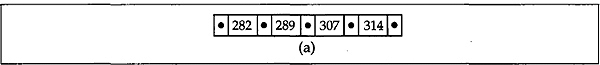
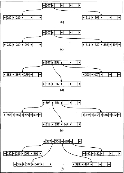
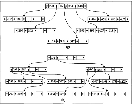
Fig. 12.18 Generation of B-tree
The basic operations that can be performed on a B-tree are the following: searching for a key in the B-tree, inserting a key into the B-tree, deleting a key from the B-tree.
The above discussion suggests an implementation of the B-tree node structure as in the following.
 #define     ATMOST….     /* Maximum number of keys in a node */
 #define    ATLEAST….     /* Minimum number of keys in a
                             node=[ATM0ST/2] */
 typedef        int          key_data;
 typedef        struct       node {
                             int n; /* Number of keys in the node */
                             key_data key[ATMOST+1];
                             struct     node *bough[ATMOST+1];
                             }          btreenode;
 typedef btreenode *btreeptr;
12.7.2 Searching for a Key in B-tree
Searching a B-tree is a generalization of searching in a BST. A function btree_lookup ( ) is presented. The input arguments to this function are as in the following.
- A key k to be searched into the B-tree.
- A pointer to the root node of the B-tree rootptr (may be a subtree of the B-tree) into which the searching is taking place.
The function returns the pointer to the node where the search is found or NULL if search is not found. If the search is found, the position of the key in the node is given by position, the last argument to the function and is a pointer to integer. Unlike BST search, the B-tree search method must search for the key in a node extensively. This node searching is done in another function, namely, node_search ( ). If the key is not found in the node, it must guide the search through a proper descendant of the node and so on. The function btree_lookup ( ) presented is a recursive function and uses the function node_search ( ). If node_search ( ) finds the key in the node, it returns TRUE(l), otherwise returns FALSE(0). In case the key is not present in the node, node_search ( ) sets the pointer to integer position to point to that index of the bough array of the node through which we get the right descendant so that the search can be continued. For a B-tree of large order this function node_search ( ) may be changed a little to use binary search within the node instead of sequential search. The function btree_lookup ( ) together with node_search ( ) is given in example 12.11 below.
Example 12.11
 btreeptr btree_lookup(key_data k, btreeptr rootptr, int *position)
 {
      if (rootptr == NULL)
            return NULL;
      else if (node_search(k, rootptr, position))
            return rootptr;
      else
            return btree_lookup(k, rootptr->bough[*position].position);
 }
 int  node_search(key_data k, btreeptr ptr, int *pos)
 {
      if (k < ptr->key[1])
      {
            *pos = 0;
            return 0; /* Return FALSE */
      }
      else  { /* Sequential search within the node follows */
            *pos = ptr->n;          /* Set the last index */
            while (k < ptr->key[*pos] && *pos>1)
                  (*pos)- -;
            return ( (k == ptr->key[*pos])?1:0 );
      }
}
12.7.3 Inserting a Key into B-tree
Inserting a key into the B-tree is extensively discussed earlier in this section where we considered the generation of a B-tree. We have already seen that as we insert nodes in a BST, it grows at the leaf. Unlike BSTs, a B-tree grows at the root as we insert keys into it. This growing at the root is mainly because of the property that all the leaves are at the same level in a B-tree. In general, when a record with known keys is to be inserted into a B-tree, first the key is to be searched into the tree using a process like btree_lookup ( ). If the key is already found in the tree the insertion process is skipped. Otherwise the lookup process finds the leaf (L say) into which the key should be inserted. Now, if this leaf L is not full to its capacity, then insert the record into the leaf. But if L is full to its capacity, then a new leaf (L' say) is created so that the keys in L together with the new key are distributed evenly in L and L' and the middle key is sent upwards, that is, in this situation the leaf L is split into two leaves L and L' (considering that the order n of the B-tree is odd) such that L contains the first n/2 keys, L' contains last n/2 keys, and the middle key (must be there for odd n) is inserted into the parent (if the parent is not full). The same process is continued until we reach the root.
We assume that the key to be inserted, k, is not present in the B-tree. Then the function btree_insert ( ) requires the following two arguments: k, the key to be inserted, and rootptr, the pointer to the root node of the B-tree, and the function returns the pointer to the root node of the B-tree after insertion is over.
The function btree_insert ( ) is a recursive one and may look like in the example 12.12.
Example 12.12
 btreeptr btree_insert(key_data k, btreeptr rootptr)
 {
      int moveup; /* 1 or 0 depending on height of B-tree has increased or not */
      key_data    newk; /* Key to be reinserted as new root node */
      btreeptr    newkr; /* Pointer to right subtree of newk */
      btreeptr    ptr; /* An auxiliary pointer */
      moveup = movedown(k, rootptr, &newk, &newkr);
      if (moveup)
      {
            ptr = (btreeptr)malloc(sizeof(btreenode));
            ptr->n = 1;
            ptr->key[1] = newk;
            ptr->bough[0] = rootptr;
            ptr->bough[1] = newkr;
            return ptr;
      }
      return rootptr;
}
Note that the function btree_insert ( ) calls the function movedown ( ) which is used to search for the key k in the B-tree pointed by rootptr to find its insertion point. This function uses four arguments as given below.
- Key k to be searched in the B-tree for insertion.
- ptr, the pointer to the root node of the subtree in which the search takes place.
- pm, pointer to the key to be inserted into a newly created root (in case of splitting).
- pmr, pointer to the new node (the right subtree of pm) after splitting.
The function movedown ( ) returns TRUE when the key pointed by pm is to be placed in a new root node, and the height of the entire tree increases. When the height of the tree does not increase, the function returns FALSE. In such a situation the function movedown ( ) inserts the key into the proper node of the B-tree, if required, movedown ( ) is a recursive function and it terminates when ptr, the pointer to the root node of the subtree in which the search taking place, is NULL. When a recursive call to movedown ( ) returns TRUE, then an attempt is made to insert the key pointed by pm to the current node. This is straightforward if there is room for the key in the current node. Otherwise, the current node *ptr splits into *ptr and *pmr and the middle key is moved upwards through the tree. The function movedown ( ) in turn uses the following three other functions.
- node search ( ), to search for a key within a node as shown earlier.
- putkey ( ), which allows to put the key into the node *ptr when possible. Actually the function is called only when *ptr has room for a key.
- split ( ), which splits the node *ptr into *ptr and *pmr.
The movedown (0) function may now be written as given shown in example 12.13.
Example 12.13
 movedown(key_data k, btreeptr      ptr, key_data *pm, btreeptr *pmr)
 {
      int  b;   /* On which bough to continue the search */


      if (ptr == NULL)
      {
            *pm = k;
            *pmr = NULL;
            return TRUE;
      }
      else  {
            if ( !nodesearch(k, ptr, &b))
                  if (movedown(k, ptr->bough[b], pm, pmr))
                      if (ptr->n < ATMOST)
                      {
                            putkey(*pm, *pmr, ptr, b);
                            return FALSE;
                      }
                      else  {
                            split(*pm, *pmr, ptr, b, pm, pmr);
                            return TRUE;
                      }
          return FALSE;
      }
 }
The function putkey ( ) puts a key into a node *ptr after making room at a proper index within the node and also sets the pointer to its branches at correct position. This may be written as in example 12.14.
Example 12.14
 putkey(key_data k, btreeptr pmr, btreeptr ptr, int pos)
 {
      int   c;


      for(c=ptr->n; c>pos; --c)
      {
            ptr->key[c+1] = ptr->key[c];
            ptr->bough[c+1] = ptr->bough[c];
      }
      ptr->key[c+1] = k;
      ptr->bough[c+1] = pmr;
      ++ptr->n;
 }
Finally, the split ( ) function splits the node *ptr with key k and pointer pmr at position pos into nodes *ptr and *qmr with middle key m. Clearly, the key k cannot be inserted directly into a node with full capacity. So we must first determine whether k will go to the left or right half, split the node accordingly, and then insert k at its correct place. During the process the middle key m is stored in the left half. The function spli t ( ) is shown in example 12.15.
Example 12.15
 split(key_data k, btreeptr pmr, btreeptr ptr, int pos,
      key_data *m, btreeptr *qmr)
 {
      int  c, mid;
      mid = (pos <= ATLEAST)? ATLEAST: ATLEAST+1;
      *qmr = (btreeptr)malloc(sizeof(btreenode));
      for(c=mid+1; c<=ATMOST; ++c)
      {
            (*qmr)->key[c-mid] = ptr->key[c];
            (*qmr)->bough[c-mid] = ptr->bough[c];
      }
      (*qmr)->n = ATMOST-mid;
      ptr->n = mid;
      (pos <= ATLEAST)? putkey(k, pmr, ptr, pos)
                 : putkey(k, pmr, *qmr, pos-mid);
      *m = ptr->key[ptr->n];
      (*qmr)->bough[0] = ptr->bough[ptr->n];
      ptr->n--;
      return;
 }
12.7.4 Deleting a Key from B-tree
The deletion of a key from B-tree is even more complex than insertion of a key in it. We discuss the deletion process through an example for a better understanding. This is shown in Fig. 12.19 in a step-by-step manner. Consider that we have a B-tree as shown in Fig. 12.18((h) which we generated earlier. Firstly, let us delete the key 337 from it. This deletion is simple because the leaf node containing the key 337 is having more than the minimum number of keys in it. What we do is, simply place its successor key 347 into the place of 337 as shown using a dashed arrow in Fig. 12.19((a) and shift the other keys in the node accordingly. Next, we delete the key 448 from the B-tree. Note that, in this case we are going to delete from a non-leaf node. We therefore move the immediate successor of this key, which is 462, into this position and then delete 462 from the node containing it, which is a leaf, as earlier. The key movement from place to place is also shown with dashed arrows in Fig. 12.19((a). After these deletions the tree takes the form as in Fig. 12.19((b). Now let us consider the case where we try to delete a key from a leaf node which is having minimum number of keys in it. This means that a key deletion from this node will leave its node with too few keys. Consider that we have to delete the key 436 from its node. This situation is tackled in the following way. Notice that its successor 462 is in its parent node. Therefore 462 is moved down to take the place of 436 and is removed (deleted) from its original place as earlier, that is, its original place is replaced by its successor 468 and 468 is deleted from its leaf node. The process of deletion is depicted in Fig. 12.19((b). The deletion of the key 299 needs special attention. Notice that the deletion of 299 leaves its leaf node with too few keys. Moreover, neither of its siblings can spare a key for this leaf. Therefore, the node is combined with one of its siblings together with the middle key from its parent node as shown with the loop in Fig. 12.19((c). After combining, the configuration of the B-tree is shown in Fig. 12.19((d). A careful look at this figure tells us that the effect of combining will leave the parent node with too few keys, and again its sibling cannot spare a key for it. Therefore, the top three nodes are again combined to a single node as shown in Fig. 12.19((d) to yield the final B-tree after deletion which is shown in Fig. 12.19((e).
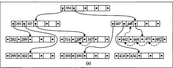
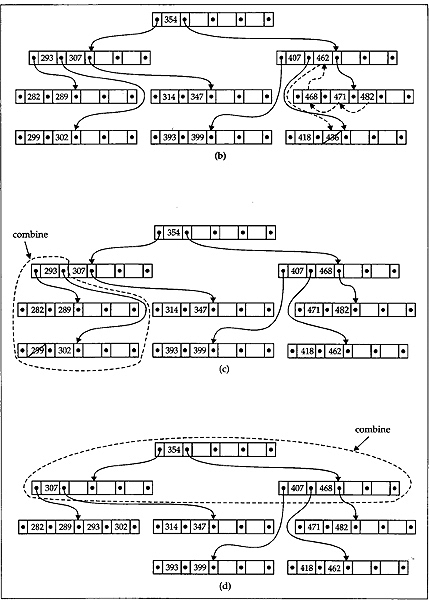
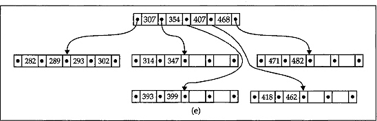
Fig. 12.19
All the cases of deletion of keys from a B-tree are discussed above in detail. We leave the development of a detailed program for deleting a key from B-tree to the reader.
E![]() X
X![]() E
E![]() R
R![]() C
C![]() I
I![]() S
S![]() E
E![]() S
S
- For each node in the tree in Fig. 12.7
(i) Name the parent node
(ii) List the children
(iii) List the siblings
(iv) Find the depth and height of the tree
- Define binary tree and binary search tree and distinguish between them.
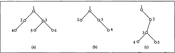
- Give the visiting sequence of vertices of each of the following binary trees under
(i) Preorder
(ii) Inorder
(iii) Postorder traversal
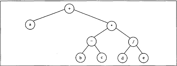
- Find the prefix, infix, and postfix expressions corresponding to the tree shown below.
- (a) Show the tree after inserting the following integers in sequence into an initially empty binary search tree (BST).
18 6 20 25 32 8 12 16
(b) Show the BST after deleting the root from your BST.
- Construct a binary tree, given the preorder and inorder sequences as below.
preorder: a b c e i f j d g h k l
inorder: e i c f j b g d k h l a
- Show that in a binary tree with n nodes, there are (n+1) NULL pointers representing children.
- Show that the number of leaves in a non-empty binary tree is equal to the number of full nodes plus one, where a full node is a node with two non-empty children.
- How does a binary search tree, (BST) differ from an AVL tree and in what situation a BST is inefficient as compared to an AVL tree with respect to searching time?
- What is a threaded binary tree and what is its main advantage over an ordinary binary tree?
- Write a function to generate the AVL tree of height h with minimum number of nodes in it.
- Write a routine to perform deletion from a B-tree.