
13
GRAPHS
13.1 INTRODUCTION
Graphs are the most common ‘abstract’ structures encountered in computer science. Any system that consists of discrete states or sites (called nodes or vertices) and connections between them can be modeled by a graph. In computer science, mathematics, engineering, and many other disciplines we often need to model a symmetric relationship between objects. The objects are represented by nodes and the connections between nodes of a graph are called edges (in case the connections are between ordered pair of nodes), or directed edges (in case the connections are between ordered pairs of nodes). Connections may also carry additional informations as labels or weights related to the interpretation of the graph. Consequently, there are many types of graphs and many basic notions that capture aspects of the structure of graphs. Also, many applications require efficient algorithms that essentially operate on graphs.
Graphs occur often in real life, and we encounter them in natural situations. For example, a road map showing the interstate highway connections between cities is an excellent example of an undirected graph, since all interstate highways are two-way. We could also add weights to each edge to indicate the distance in miles between the two cities, producing a weighted undirected graph.
The sequence of courses that one must take to complete a degree in computer science can also be represented as a graph. It is a directed graph in which the direction or edge implies the specific order in which the course must be taken.
Another example that is a little more closely related to computer science is the graph that represents resource allocations. It describes the relationship between a process, that is, a program in execution and other resources in the system such as memory, a file, or printer. A resource allocation graph is a directed graph with edges going from a process node to a resource node.
In a computer network, computers are interconnected via high-speed communication channels such as phone line, optical fibres, microwave relays, or satellites. We can use a graph-based representation to determine how to route messages from one node to another and to find backup routes in case of node.
Graphs are frequently applied in diverse areas such as artificial intelligence, cybernetics, chemical structures of crystals, transportation networks, electrical circuitry, and the analysis of programming languages.
In this chapter we give graph representation and traversal algorithms. We also describe the details of the carefully tuned data structures that may be needed to achieve the ultimate bounds on time and space complexity for the algorithms.
13.2 GRAPH FUNDAMENTALS
When a computational problem is modeled in terms of graphs, the resulting graphs must be generated and represented in some form in order to facilitate the operations of an algorithm. The desired representation may be an ‘abstract’ data structure that supports certain operations very efficiently, or it may be a ‘concrete’ display or drawing of the graph that allows visual inspection and interactive manipulation.
A graph is the most generalized of all data representation. A graph structure is a generalization of a hierarchical structure. The essence of a hierarchical structure is that each of its components, with a few exceptions, has a unique predecessor and a bounded number of successors. In a graph, each component may be related to any other component. Thus a graph is a (many:many) data structure in which each component of the graph can have an arbitrary number of successors and an arbitrary number of predecessors.
A graph is a structure G={V, E} in which V is a finite set of nodes and E is a finite set of edges. We will denote nodes by drawing a circle around a node identifier and edges by using line segments. A graph is a simple graph if it has no self-loop and parallel edges.
An edge connects two nodes. If the edges have a direction associated with them, then the graph is called a directed graph or sometimes a digraph. If there is an edge between nodes ni and nj in a directed graph, then ni is called the tail of the edge and nj is called the head of the edge. We also say that ni is adjacent to or incident to node nj. The neighbours of a node are all nodes that are adjacent to it.
If no direction is associated with an edge, then the graph is called undirected graph. The presence of an edge implies that there exist connections in each direction.
Fig. 13.1 and 13.2 show the structures of both directed graph and undirected graph.
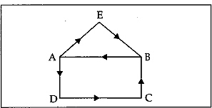
Fig. 13.1 Directed graph
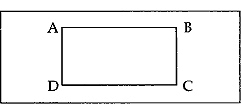
Fig. 13.2 Undirected graph
Note that in an undirected graph there can be at the most n(n-1)/2 edges for n nodes.
A weighted graph is a graph in which each edge has an associated value. A weighted edge has a scaler value W associated with it. The weight is a measure of the cost of using this edge to go from source node to destination.
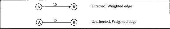
Fig. 13.3 Weighted edge for directed and undirected graphs
A city map showing only the one-way streets is an example of a digraph where nodes are the intersection of streets and the edges are the streets. Two-way streets in an example of an undirected graph.
Any sequence of edges of a directed graph such that the terminal node of any node in the sequence is the initial node of the edge, if any, appearing next in the sequence defines a path of the graph. In other words, a simple path through a graph is a sequence of vertices V1 V2,…, Vk such that all vertices except possibly the first and the last, are distinct and each pair or nodes Vi, Vi=1, i=1, k-1 is connected by an edge. Consider Fig. 13.4.
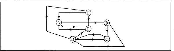
Fig. 13.4 Directed graph showing path
In the above figure, the sequence ABCD is a simple path. DFABCD is also a path. However, ABE is not a path since there is no edge directly connecting nodes B and E. BCDBC is also not a path since all nodes are not distinct (the nodes B and C appear twice in the sequence).
A cycle or circuit is a simple path V1, V2, V3,…, Vk exactly as defined above but with the added requirement that V1 =Vk.
For example, CDC and ABCDFEA are cycles. A cycle is called a simple cycle if no edges appear more than once, otherwise it is a cycle.
The outdegree of a node in a directed graph is the number of edges exiting from the node; the indegree of a node is the number of edges entering the node. In the following figures, the indegree of CALCUTTA is 2 and its outdegree is 1. The indegree and outdegree of NEW DELHI are 2 and 2, respectively .The indegree and outdegree of a node in a directed graph indicate its relative importance of that graph. A node whose outdegree 0 acts primarily as a sink node and a node whose indegree is 0 is called a source node.
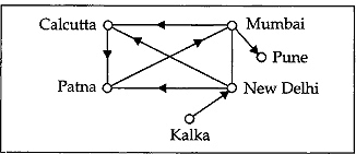
Fig. 13.5 Directed graph
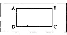
Fig. 13.6 Undirected graph
For example, in the figure, KALKA is the source node and PUNE is the sink node. Since indegree and outdegree cannot apply to a node in an undirected graph, the degree of a node is defined as the number of edges connected directly to the node. In Fig. 13.6 the degree of each node is 2.?
13.3 GRAPH REPRESENTATION
A graphical representation of graph has a limited usefulness. There are various popular approaches for representing graph structures. We will consider only two basic approaches— adjacency matrix and adjacency list. The method of matrix representation has a number of advantages. It is easy to store and manipulate matrices and hence the graphs, represented by them, are processed by computer. Matrix algebra can be used to obtain paths, cycles, and other features of a graph.
13.3.1 Adjacency Matrix
The adjacency matrix A for a graph G of n nodes is an n x n matrix. Any element of the adjacency matrix is either 0 or 1. We set Aij = 1 if there is an edge from Vi to Vj, and Aij = 0 if there is no such edge. It is mathematically written as
Aij =1 if there is an edge from Vi to Vj
= 0, otherwise
The above matrix is also called a bit matrix or a boolean matrix. The ith row in the adjacency matrix is determined by the edge that originates in the node Vj Fig. 13.7 shows the graph and the corresponding adjacency matrix.
Since we are using only simple graph (i.e., no self-loop and parallel edges), the adjacency matrix has zeros on its main diagonal, that is, Aii = 0, for 1 ≤ i ≤ n. (i.e., A11 = 0, A22= 0 and so on).
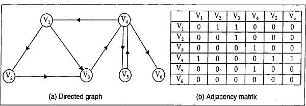
Fig. 13.7
Similarly, we can draw adjacency matrix of an undirected graph. The adjacency matrix and the corresponding graph for an undirected graph are shown in the figures below.
Fig. 13.8 Undirected graph
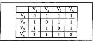
Fig. 13.9 Adjacency matrix?
The adjacency matrix for an undirected graph is always symmetric whereas the adjacency matrix for a directed graph need not be symmetric. In other words, if the graph is undirected, then A (i, j)=A(j, i) for all i, j.
13.3.2 Adjacency Lists
The adjacency list is a potentially more space-efficient method for representing graphs. Fig. 13.10(b) is an adjacency-list representation of the undirected graph G in Fig. 13.10(a). Similarly, Fig. 13.10(b) is an adjacency-list representation of the directed graphs G1 in the figure. The corresponding adjacency matrices are shown in Fig. 13.10(c) and Fig. 13.10(c). The symbol ‘/’ indicates end of the corresponding list.
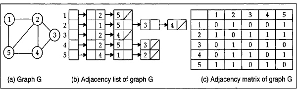
Fig. 13.10
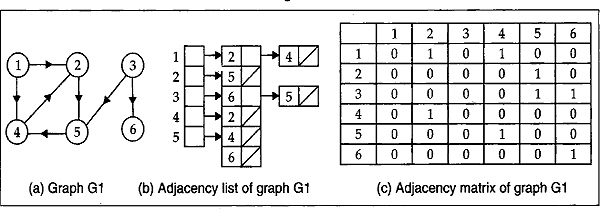
Fig. 13.11
In adjacency list representation, we store all the vertices in a list and then for each vertice, we have a linked list of its adjacency vertices. In the next section, the graph traversal algorithm will be discurssed.
13.4 GRAPH TRAVERSAL
Graph search is the analogue of graph traversal. In many practical applications of graphs, there is a need to visit systematically all the vertices of a graph. One such application occurs when the organizers of a political campaign want to make a list of all important political centres for their candidate to visit. The presence or absence of edges between such centres will determine the possible ways through which all the centres could be visited. Two standard ways of searching a graph are breadth-first search and depth-first search. In the next two subsections we shall investigate the methods that ensure that all nodes are visited.
13.4.1 Breadth-first Search
Breadth-first search is one of the simplest algorithms for searching a graph. Although it can be used both for directed and undirected graphs, we shall describe it in relation to undirected graphs.
Given a graph G=(V, E) and a distinguished source vertex V, breadth-first search systematically explores the edges of G to discover every vertex that is reachable from V. It begins at a given node and then proceeds to all nodes directly connected to that node. The following steps are involved in the algorithm.
Algorithm 13.1: Breadth-first search
A graph, G, is either directed or undirected graph and is represented by an adjacency matrix.
Step 1: Start with any vertex and mark it as visited.
Step 2: Using the adjacency matrix of the graph, find a vertex adjacent to the vertex in step 1. Mark it as visited.
Step 3: Return to the vertex in Step 1 and move along an edge towards an unvisited vertex, and mark the new vertex as visited.
Step 4: Repeat Step 3 until all vertices adjacent to the vertex, as selected in Step 2, have been marked as visited.
Step 5: Repeat Step 1 through Step 4 starting from the vertex visited in Step 2, then starting from the nodes visited to Step 3 in the order visited. If all vertices have been visited, then continue to next step.
Step 6: stop
In a breadth-first search, the graph is searched breadthwise by exploring all the nodes adjacent to a node. A queue is a convenient data structure to keep track of nodes that are visited during a breadth-first search.
The following program implements the breadth-first algorithm as described earlier.
Example 13.1
— — — — — — — — — — — — — — — — — — — — — — —
Searching all the vertices of an undirected graph that can be reached by a specific vertex in the same graph by the Breadth-first search method
— — — — — — — — — — — — — — — — — — — — — — —
      #include <stdio.h>
      #include <stdio.h>
      void insert (int);
      int queue[20], rear=-1, graph[7][7], row ;
      void insert (int x)
      {

           rear= rear+1;
           queue[rear]=x ;
      }
      Remove( )
      {

           int item, k;
           item= queue[0];
           for(k=0, k<rear; k++)
                 queue[k]= queue[k+1];
           rear = rear-1;
           return(item);
      }
      void main( )
      {

           int i, j , num, w, visited[10], v, j1;
           int 1, vertices[10], count=0, final[10];
           clrscr( );
           randomize( );
           printf(“How many vertices are there ====>”);
           scanf(“%d”, & row);
           printf(“
 The graph's adjacency matrix is as follows:


”);
           printf(“      ”);
      for(j=0, j<row; j++)
           printf(“Vertex %d
”, j);
      for(i=0, i<row; i++)
      {

           for(j=count; j<row; j++)
      {
                  if(i ! =j)
                  {
           graph[i][j] = random (2);
           graph[j] [i] = graph [i] [j];
           }
           else graph[i][j] =0 ;
      }

           count++;
      }
      for (i=0; i<row; i++)
      {
           printf(“Vertex %d”, i);
           for(j=0; j<row, j++)
           printf(“%8d”, graph[i][j]);
           printf(“

”);
      }
      for (i=0; i<row, i++)
           visited[i]= 0;
      printf(“
 Enter the vertex number from which to start ====>”);
      scanf(“%d”, &v);
      visited[v]= 1;
      insert(v);
      getch( );
      clrscr( );
      printf(“
 Starting vertex = = = > Vertex %d

”, v);
      count=1;
      j1 = 0;
      while(rear>=0)
      {

           v=Remove( );
           final[j1]=v;
           j1++;
           1 = 0;
           for(i=0; i<row; i++)
           if(graph[v][i]==1)
           {
           vertices[1]=i;
               1 + +;

           }
           for(i=0; i<1 i++)
           {
                 w=vertices[i];
                 printf(“Step %d: Vertex visited = = = > Vertex
                 %d
”, count, w);
                 if(visited[w]!=1)
                      {
                      insert(w);
                      visited[w]=1;
                      }

           }
           printf(“Elements in the queue ===>”);
           if(rear>=0)
           for(J=1; j<=rear; j++)
             printf (“%d”, queue[j]);
      else

           printf(“EMPTY QUEUE: TRAVERSAL COMPLETE”);
           count++;
           printf(“


”);
           getch( );
           clrscr( );
           }
           printf(“
 The vertices that are traversed”);
           printf(“from vertex %d are as follows:
”, v);
           if(count==2)
                 printf(‘
 Vertex %d: Is an isolated vertex", v);
           else
                 for(i=o); i<j1; i++)
                   printf(“Vertex %d,”, final[i]);
           getch( );
      }
The program produces the following output corresponding to the given input.
How many vertices are there = = => 5
The graph's adjacency matrix is as follows:
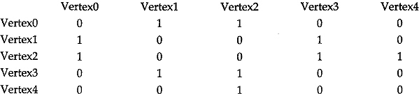
Enter the vertex number from which to start = = = =>3
Starting vertex = = = => Vertex3
Step1: Vertex visited = = = => Vertex1
Step1: Vertex visited = = = => Vertex2
Elements in the queue = = = => 1,2,
Step2: Vertex visited = = = ==> Vertes 0
Step2: Vertex visited = = = ==> Vertex 3
Elements in the queue = = => 2,0,
Step3: Vertex visited = = => Vertex0
Step 3: Vertex visited = = = => Vertex3
Step 3: Vertex visited= = = => Vertex4
Elements in the queue = = => 0,4,
Step 4: Vertex visited = = = => Vertex1
Step 4: Vertex visited = = = => Vertex2
Elements in the queue = = = => 4,
Step 5: Vertex visited = = = => Vertex2
Elements in the queue = = = => EMPTY QUEUE: TRAVERSAL COMPLETE
The vertices that are traversed from vertex3 are as follows
Vertex3, Vertex1, Vertex2, Vertex0, Vertex4, 13.4.2
13.4.2 Depth-first Search
Depth-first search (DFS) can be described in a manner analogous to breadth-first search. The main difference is the use of a stack instead of a queue.
In a DFS, initially all nodes in a graph are marked unvisited. Select any node, say Vo, in the graph and proceed in the following way whenever a node Vi is reached. When Vi was not reached before, mark it as visited. If there are no unexplored edges left in the edge list of Vi, then backtrack to the node from which Vi was reached. Otherwise traverse the first unexplored edge (i, j) in the edge list of i. When j was visited before mark the edge and backtrack to i. When j was not visited before, mark the edge. Now ‘visit’ the node reached in a similar manner.
A depth-first graph traversal algorithm utilizing the above approach is given below.
Algorithm 13.2: Depth-first search
A graph G is represented by an adjacency matrix. The input graph G may be undirected or directed.
Step 1: Choose an arbitrary node in the graph, designate it as the search node, and mark it as visited.
Step 2: From the adjacency matrix of the graph, find a node adjacent to the search node that has not been visited as yet. Mark it as visited new search node.
Step 3: Repeat Step 2 using the new search node If there are no nodes satisfying on Step 2, return to the previous search node and continue the process from there.
Step 4: When a return to the previous search node in Step 3 is impossible, the search from the original chosen search node is complete.
Step 5: If there are any nodes in the graph which are still unvisited, choose any node that has not been visited and repeat Step 1 through Step 4.
Step6: stop
A connected component of graph G (not directed) is a maximal connected subgraph, that is, a connected subgraph that is not contained in any large connected subgraph. The problem of finding the connected components of a graph can be solved by using depth-first search with very little modification. We may start with an arbitrary vertex, do a depth-first search to find all other vertices (and edges) in the same component one after, if same vertices remain, choose one and repeat.
In case of depth–first search, stack is the convenient structure to implement the depth–first search.
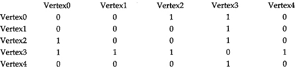
Illustration: Consider the directed graph and the corresponding adjacency matrix shown in Fig. 13.12(a) and Fig. 13.12(b). Although we will illustrate the depth-first search algorithm for a directed graph, the approach can also be applied to undirected graphs.
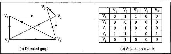
Fig. 13.12
Let us choose V1 as the starting node in the graph. First designate it as the search node and mark it as visited. The nodes V2 and V3 are adjacent to V1 Next we will mark V2 for searching the possible path. There is no node adjacent to V2 and we move to V1 again for considering the next possibility of node, that is, V3. All nodes adjacent to V3 also have been visited. So we will return to V1. The search from V1 is now completed since all nodes except V4 and V5 have been visited.
We now choose V4 first and mark it as visited. Since V5 is the only unvisited node adjacent to V4 proceed to V5. V2 is the only node adjacent to V5 we will move to V2 that has already been visited. Then we will return to V4 and the total search is complete.
Depth-first search is a generalization of traversing trees in preorder. The starting vertex may be determined by the problem or may be chosen arbitrarily. While traversing vertices starting from the initial vertex, a dead end may be reached. A dead end is a vertex such that all its neighbours, that is, vertices adjacent to it, have already been visited. At a dead end we back up along the last edge traversed and branch out in another direction. The beauty of the depth-first algorithm, developed by J E Hopcroft and R E Tarjan, lies in the idea that the algorithm is used to develop many important algorithms.
In a breadth-first search, vertices are visited in order of increasing distance from the starting vertex, say V, where distance is simply the number of edges in a shortest path. An efficient implementation for either method must keep a list of vertices that have been visited but whose adjacent vertices have not yet been visited. The depth-first search backs up from a dead end, it is supposed to branch out from the most recently visited vertex before pursuing new paths from vertices that were visited earlier. Thus the list of vertices from which some paths remain to be traversed must be in a stack. On the otherhand, in a breadth-first search, in order to ensure that vertices close to V are visited first the list must be a queue.
The following C program implements the depth-first algorithm.
Example 13.2
— — — — — — — — — — — — — — — — — — — — — — —
Searching all the vertices of an undirected graph that can be reached from a specific vertex, by the Depth-first search method
— — — — — — — — — — — — — — — — — — — — — — —
      #include <stdio.h>
      #include <stdio.h>
      struck stack
      {
            int data[20];
            int top;
      };
      void push(struct stack*, int);
      int graph[10][10], row;


      void main( )
      {
            struct stack S ;
            int i, j, count=0, v, visited[15];
            int 1, vertices[15], w, final[15], index=0;
            clrscr( );


            randomize( );
            printf(“How many vertices are there ====>”);
            scanf(“%d”, &row);
            printf(“
 The graph's adjancency matrix is as follows:


”);
            printf(“   ”);
            for(j=0; j<row; j++)
            printf(“Vertex %d”, j);
            printf(“
”);
            for(i=0; i<row; i++)
            {
            for(j=count; j<row; j++)
               {

                    if (i!=j)
                    {
                    graph[i][j]=random(2);
                    graph[j][i]=graph[i][j];
                    }
                    else
                    graph[i][j]=0;
               }
               count++;
               }
               for(i=0; i<row; i++)
               {

                    printf(“Vertex %d”, i);
                    for(j=0; j<row; j++)
                    printf(*%8d', grapn[i][j];
                    printf(“

”);
               }
               for(i=0; i<20; i++)
                    S.data[i]=0;
      S.top=-1;
      printf(“Enter the vertex from which traversal starts ===>”);
      scanf(“%d”, &v);
      getch( ); clrscr( );
      for(i=0, i<row; i++)
      visited[i]=0;
      visited[v]=1;
      push(&s, v);
      printf “
 Starting vertex ====> vertex %d

”, v);
      count=1;
      while(S.top==o)
      {
      v=pop(&S);
      final[indx]=v;
      indx++;
      1 = 0;
      for(i=0, i>row i++)
      if(graph[v][i]==1)
      {
      vertices[1]= i;
        1++;

     }
     for(i=1-1; i>-0; i--)
     {
     w= vertices[1];
     printf(“step%d: Vertex visited ===> Vertex %d
”, count, w);
     if(visited [w]!=1)
           {

                 push(&S, w);
                 visited[w]=1;
           }
     {
     printf(“Elements in the stack ====>”);
     if(S.top>=0)
           for(j=0; j<=s.top; j++)
                 printf(“%d,” S.datatj]);
     else
           printf(“EMPTY STACK: TRAVERSAL COMPLETE”)
     getch( ); clrscr( );
     count++;
     }
     printf(“The traversal of the vertices by depth-first”);
     printf(“search is as follows:

”);
     for(i=0; i<indx; i++)
           printf (“Vertex %d,” final[i]);
     getch( );
     }
     void push(struct stack *s1, int x)
     {
     s1->top=s1->top+1;
     s1->data[s1->top]=x;
     }
     pop(struct stack *s1)
     {
     int p;
     p=s1->data[s1->top];
     s1->top=s1->top-1;
     return(p);
     }
The program produces the following output corresponding to the given input:
How many vertices are there = = = => 5
The graph's adjacency matrix is as follows:
Enter the vertex from which traversal starts = = =>2
Starting vertex = = => vertex2
Step 1: Vertex visited = = => Vertex3
Step 1: Vertex visited = = => Vertex 0
Elements in the stack = = => 3,0,
Step 2: Vertex visited = = = => Vertex3
Step 2: Vertex visited = = = => Vertex2
Elements in the stack = = = => 3,
Step 3: Vertex visited = = = => Vertex4
Step 3: Vertex visited = = = => Vertex2
Step 3: Vertex visited = = = ==> Vertex1
Step 3: Vertex visited = = = => Vertex0
Elements in the stack = = = => 4,1,
Step 4: Vertex visited = = = => Vertex3
Elements in the stack = = = => 4,
Step 5: Vertex visited = = => Vertex3
Elements in the stack = = => EMPTY STACK: TRAVERSAL COMPLETE
The traversal of the vertices by depth-first search is as follows:
Vertex2, Vertex0, Vertex3, Vertex1, Vertex4
E![]() X
X![]() E
E![]() R
R![]() C
C![]() I
I![]() S
S![]() E
E![]() S
S
- Describe the adjacency matrix representation of graph. What are its advantages and disadvantages?
- What are the main advantages of adjacency list representation of a graph over the adjacency matrix representation?
- Explain the difference between directed graph and undirected one?
- Write a pseudo code to implement the Breadth-first search algorithm.
- Consider a graph in which the relationship among the nodes is linear. Describe the order in which the nodes will be processed during Depth-first search that start at one of the nodes with only one neighbour. What happens if the search starts at one of the nodes with two neighbour?
- Both Breadth-first and Depth-first search procedures probe each node in the graph at least once and each edge twice. Prove that this effort is O(ne+n), where n is the number of nodes and e denotes the number of edges.
- Write a recursive routine to implement Breadth-first search.
- Write an algorithm to produce the shortest path from a node m to another node n in an undirected graph if a path exists, or an indication that no path exists between two nodes.
- Let D be a directed graph and TD be the directed graph formed by adding an edge from d1 to d2 whenever d2 and d2 (with no direct edge) are nodes in D and there is a path from d1 to d2. TD is the transitive closure of D. Write an algorithm to compute the transitive closure of a digraph.
- A topological order is a linear relationship among the nodes of a directed graph such that each directed edge goes from a node to one of its successors. The basic idea behind topological sorting is to find a node with no successor, remove it from the graph and add it to a list. Repeat this process until the graph is empty. Write an algorithm to implement topological sorting.
- Explain briefly the following terms:
a. diagraph b. adjacency list c. Traversal of graph