LSM Tree Structure

We start with ordered LSM Trees [ONEIL96], where files hold sorted data records. Later, in “Unordered LSM Storage”, we’ll also discuss structures that allow storing data records in insertion order, which has some obvious advantages on the write path.

As we just discussed, LSM Trees consist of smaller memory-resident and larger disk-resident components. To write out immutable file contents on disk, it is necessary to first buffer them in memory and sort their contents.

A memory-resident component (often called a memtable) is mutable: it buffers data records and serves as a target for read and write operations. Memtable contents are persisted on disk when its size grows up to a configurable threshold. Memtable updates incur no disk access and have no associated I/O costs. A separate write-ahead log file, similar to what we discussed in “Recovery”, is required to guarantee durability of data records. Data records are appended to the log and committed in memory before the operation is acknowledged to the client.

Buffering is done in memory: all read and write operations are applied to a memory-resident table that maintains a sorted data structure allowing concurrent access, usually some form of an in-memory sorted tree, or any data structure that can give similar performance characteristics.

Disk-resident components are built by flushing contents buffered in memory to disk. Disk-resident components are used only for reads: buffered contents are persisted, and files are never modified. This allows us to think in terms of simple operations: writes against an in-memory table, and reads against disk and memory-based tables, merges, and file removals.

Throughout this chapter, we will be using the word table as a shortcut for disk-resident table. Since we’re discussing semantics of a storage engine, this term is not ambiguous with a table concept in the wider context of a database management system.

Two-component LSM Tree

We distinguish between two- and multicomponent LSM Trees. Two-component LSM Trees have only one disk component, comprised of immutable segments. The disk component here is organized as a B-Tree, with 100% node occupancy and read-only pages.

Memory-resident tree contents are flushed on disk in parts. During a flush, for each flushed in-memory subtree, we find a corresponding subtree on disk and write out the merged contents of a memory-resident segment and disk-resident subtree into the new segment on disk. Figure 7-1 shows in-memory and disk-resident trees before a merge.

Figure 7-1. Two-component LSM Tree before a flush. Flushing memory- and disk-resident segments are shown in gray.

After the subtree is flushed, superseded memory-resident and disk-resident subtrees are discarded and replaced with the result of their merge, which becomes addressable from the preexisting sections of the disk-resident tree. Figure 7-2 shows the result of a merge process, already written to the new location on disk and attached to the rest of the tree.

Figure 7-2. Two-component LSM Tree after a flush. Merged contents are shown in gray. Boxes with dashed lines depict discarded on-disk segments.

A merge can be implemented by advancing iterators reading the disk-resident leaf nodes and contents of the in-memory tree in lockstep. Since both sources are sorted, to produce a sorted merged result, we only need to know the current values of both iterators during each step of the merge process.

This approach is a logical extension and continuation of our conversation on immutable B-Trees. Copy-on-write B-Trees (see “Copy-on-Write”) use B-Tree structure, but their nodes are not fully occupied, and they require copying pages on the root-leaf path and creating a parallel tree structure. Here, we do something similar, but since we buffer writes in memory, we amortize the costs of the disk-resident tree update.

When implementing subtree merges and flushes, we have to make sure of three things:

1. As soon as the flush process starts, all new writes have to go to the new memtable.

2. During the subtree flush, both the disk-resident and flushing memory-resident subtree have to remain accessible for reads.

3. After the flush, publishing merged contents, and discarding unmerged disk- and memory-resident contents have to be performed atomically.

Even though two-component LSM Trees can be useful for maintaining index files, no implementations are known to the author as of time of writing. This can be explained by the write amplification characteristics of this approach: merges are relatively frequent, as they are triggered by memtable flushes.

Multicomponent LSM Trees

Let’s consider an alternative design, multicomponent LSM Trees that have more than just one disk-resident table. In this case, entire memtable contents are flushed in a single run.

It quickly becomes evident that after multiple flushes we’ll end up with multiple disk-resident tables, and their number will only grow over time. Since we do not always know exactly which tables are holding required data records, we might have to access multiple files to locate the searched data.

Having to read from multiple sources instead of just one might get expensive. To mitigate this problem and keep the number of tables to minimum, a periodic merge process called compaction (see “Maintenance in LSM Trees”) is triggered. Compaction picks several tables, reads their contents, merges them, and writes the merged result out to the new combined file. Old tables are discarded simultaneously with the appearance of the new merged table.

Figure 7-3 shows the multicomponent LSM Tree data life cycle. Data is first buffered in a memory-resident component. When it gets too large, its contents are flushed on disk to create disk-resident tables. Later, multiple tables are merged together to create larger tables.

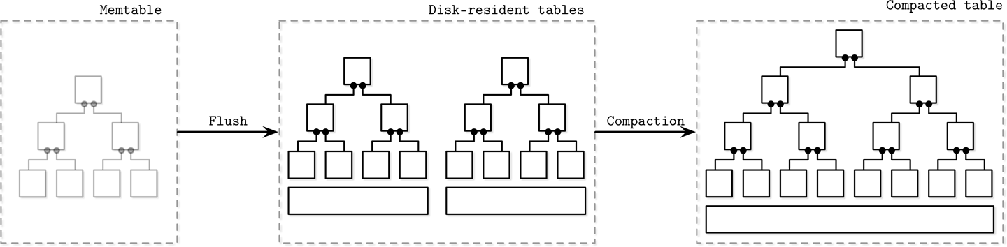
Figure 7-3. Multicomponent LSM Tree data life cycle

The rest of this chapter is dedicated to multicomponent LSM Trees, building blocks, and their maintenance processes.

In-memory tables

Memtable flushes can be triggered periodically, or by using a size threshold. Before it can be flushed, the memtable has to be switched: a new memtable is allocated, and it becomes a target for all new writes, while the old one moves to the flushing state. These two steps have to be performed atomically. The flushing memtable remains available for reads until its contents are fully flushed. After this, the old memtable is discarded in favor of a newly written disk-resident table, which becomes available for reads.

In Figure 7-4, you see the components of the LSM Tree, relationships between them, and operations that fulfill transitions between them:

Current memtable

Receives writes and serves reads.

Flushing memtable

Available for reads.

On-disk flush target

Does not participate in reads, as its contents are incomplete.

Flushed tables

Available for reads as soon as the flushed memtable is discarded.

Compacting tables

Currently merging disk-resident tables.

Compacted tables

Created from flushed or other compacted tables.

Figure 7-4. LSM component structure

Data is already sorted in memory, so a disk-resident table can be created by sequentially writing out memory-resident contents to disk. During a flush, both the flushing memtable and the current memtable are available for read.

Until the memtable is fully flushed, the only disk-resident version of its contents is stored in the write-ahead log. When memtable contents are fully flushed on disk, the log can be trimmed, and the log section, holding operations applied to the flushed memtable, can be discarded.

Updates and Deletes

In LSM Trees, insert, update, and delete operations do not require locating data records on disk. Instead, redundant records are reconciled during the read.

Removing data records from the memtable is not enough, since other disk or memory resident tables may hold data records for the same key. If we were to implement deletes by just removing items from the memtable, we would end up with deletes that either have no impact or would resurrect the previous values.

Let’s consider an example. The flushed disk-resident table contains data record v1 associated with a key k1, and the memtable holds its new value v2:

Disk Table        Memtable
| k1 | v1 |       | k1 | v2 |

If we just remove v2 from the memtable and flush it, we effectively resurrect v1, since it becomes the only value associated with that key:

Disk Table        Memtable
| k1 | v1 |       ∅

Because of that, deletes need to be recorded explicitly. This can be done by inserting a special delete entry (sometimes called a tombstone or a dormant certificate), indicating removal of the data record associated with a specific key:

Disk Table        Memtable
| k1 | v1 |       | k1 | <tombstone> |

The reconciliation process picks up tombstones, and filters out the shadowed values.

Sometimes it might be useful to remove a consecutive range of keys rather than just a single key. This can be done using predicate deletes, which work by appending a delete entry with a predicate that sorts according to regular record-sorting rules. During reconciliation, data records matching the predicate are skipped and not returned to the client.

Predicates can take a form of DELETE FROM table WHERE key ≥ "k2" AND key < "k4" and can receive any range matchers. Apache Cassandra implements this approach and calls it range tombstones. A range tombstone covers a range of keys rather than just a single key.

When using range tombstones, resolution rules have to be carefully considered because of overlapping ranges and disk-resident table boundaries. For example, the following combination will hide data records associated with k2 and k3 from the final result:

Disk Table 1      Disk Table 2
| k1 | v1 |       | k2 | <start_tombstone_inclusive> |
| k2 | v2 |       | k4 | <end_tombstone_exclusive>   |
| k3 | v3 |
| k4 | v4 |

LSM Tree Lookups

LSM Trees consist of multiple components. During lookups, more than one component is usually accessed, so their contents have to be merged and reconciled before they can be returned to the client. To better understand the merge process, let’s see how tables are iterated during the merge and how conflicting records are combined.

Merge-Iteration

Since contents of disk-resident tables are sorted, we can use a multiway merge-sort algorithm. For example, we have three sources: two disk-resident tables and one memtable. Usually, storage engines offer a cursor or an iterator to navigate through file contents. This cursor holds the offset of the last consumed data record, can be checked for whether or not iteration has finished, and can be used to retrieve the next data record.

A multiway merge-sort uses a priority queue, such as min-heap [SEDGEWICK11], that holds up to N elements (where N is the number of iterators), which sorts its contents and prepares the next-in-line smallest element to be returned. The head of each iterator is placed into the queue. An element in the head of the queue is then the minimum of all iterators.

When the smallest element is removed from the queue, the iterator associated with it is checked for the next value, which is then placed into the queue, which is re-sorted to preserve the order.

Since all iterator contents are sorted, reinserting a value from the iterator that held the previous smallest value of all iterator heads also preserves an invariant that the queue still holds the smallest elements from all iterators. Whenever one of the iterators is exhausted, the algorithm proceeds without reinserting the next iterator head. The algorithm continues until either query conditions are satisfied or all iterators are exhausted.

Figure 7-5 shows a schematic representation of the merge process just described: head elements (light gray items in source tables) are placed to the priority queue. Elements from the priority queue are returned to the output iterator. The resulting output is sorted.

It may happen that we encounter more than one data record for the same key during merge-iteration. From the priority queue and iterator invariants, we know that if each iterator only holds a single data record per key, and we end up with multiple records for the same key in the queue, these data records must have come from the different iterators.

Figure 7-5. LSM merge mechanics

Let’s follow through one example step-by-step. As input data, we have iterators over two disk-resident tables:

Iterator 1:         Iterator 2:
{k2: v1} {k4: v2}   {k1: v3} {k2: v4} {k3: v5}

The priority queue is filled from the iterator heads:

Iterator 1:         Iterator 2:         Priority queue:
{k4: v2}            {k2: v4} {k3: v5}   {k1: v3} {k2: v1}

Key k1 is the smallest key in the queue and is appended to the result. Since it came from Iterator 2, we refill the queue from it:

Iterator 1:         Iterator 2:         Priority queue:      Merged Result:
{k4: v2}            {k3: v5}            {k2: v1} {k2: v4}    {k1: v3}

Now, we have two records for the k2 key in the queue. We can be sure there are no other records with the same key in any iterator because of the aforementioned invariants. Same-key records are merged and appended to the merged result.

The queue is refilled with data from both iterators:

Iterator 1:         Iterator 2:         Priority queue:      Merged Result:
{}                  {}                  {k3: v5} {k4: v2}    {k1: v3} {k2: v4}

Since all iterators are now empty, we append the remaining queue contents to the output:

Merged Result:
  {k1: v3} {k2: v4} {k3: v5} {k4: v2}

In summary, the following steps have to be repeated to create a combined iterator:

1. Initially, fill the queue with the first items from each iterator.

2. Take the smallest element (head) from the queue.

3. Refill the queue from the corresponding iterator, unless this iterator is exhausted.

In terms of complexity, merging iterators is the same as merging sorted collections. It has O(N) memory overhead, where N is the number of iterators. A sorted collection of iterator heads is maintained with O(log N) (average case) [KNUTH98].

Reconciliation

Merge-iteration is just a single aspect of what has to be done to merge data from multiple sources. Another important aspect is reconciliation and conflict resolution of the data records associated with the same key.

Different tables might hold data records for the same key, such as updates and deletes, and their contents have to be reconciled. The priority queue implementation from the preceding example must be able to allow multiple values associated with the same key and trigger reconciliation.

To reconcile data records, we need to understand which one of them takes precedence. Data records hold metadata necessary for this, such as timestamps. To establish the order between the items coming from multiple sources and find out which one is more recent, we can compare their timestamps.

Records shadowed by the records with higher timestamps are not returned to the client or written during compaction.

Maintenance in LSM Trees

Similar to mutable B-Trees, LSM Trees require maintenance. The nature of these processes is heavily influenced by the invariants these algorithms preserve.

In B-Trees, the maintenance process collects unreferenced cells and defragments the pages, reclaiming the space occupied by removed and shadowed records. In LSM Trees, the number of disk-resident tables is constantly growing, but can be reduced by triggering periodic compaction.

Compaction picks multiple disk-resident tables, iterates over their entire contents using the aforementioned merge and reconciliation algorithms, and writes out the results into the newly created table.

Since disk-resident table contents are sorted, and because of the way merge-sort works, compaction has a theoretical memory usage upper bound, since it should only hold iterator heads in memory. All table contents are consumed sequentially, and the resulting merged data is also written out sequentially. These details may vary between implementations due to additional optimizations.

Compacting tables remain available for reads until the compaction process finishes, which means that for the duration of compaction, it is required to have enough free space available on disk for a compacted table to be written.

At any given time, multiple compactions can be executed in the system. However, these concurrent compactions usually work on nonintersecting sets of tables. A compaction writer can both merge several tables into one and partition one table into multiple tables.

Leveled compaction

Compaction opens up multiple opportunities for optimizations, and there are many different compaction strategies. One of the frequently implemented compaction strategies is called leveled compaction. For example, it is used by RocksDB.

Leveled compaction separates disk-resident tables into levels. Tables on each level have target sizes, and each level has a corresponding index number (identifier). Somewhat counterintuitively, the level with the highest index is called the bottommost level. For clarity, this section avoids using terms higher and lower level and uses the same qualifiers for level index. That is, since 2 is larger than 1, level 2 has a higher index than level 1. The terms previous and next have the same order semantics as level indexes.

Level-0 tables are created by flushing memtable contents. Tables in level 0 may contain overlapping key ranges. As soon as the number of tables on level 0 reaches a threshold, their contents are merged, creating new tables for level 1.

Key ranges for the tables on level 1 and all levels with a higher index do not overlap, so level-0 tables have to be partitioned during compaction, split into ranges, and merged with tables holding corresponding key ranges. Alternatively, compaction can include all level-0 and level-1 tables, and output partitioned level-1 tables.

Compactions on the levels with the higher indexes pick tables from two consecutive levels with overlapping ranges and produce a new table on a higher level. Figure 7-6 schematically shows how the compaction process migrates data between the levels. The process of compacting level-1 and level-2 tables will produce a new table on level 2. Depending on how tables are partitioned, multiple tables from one level can be picked for compaction.

Figure 7-6. Compaction process. Gray boxes with dashed lines represent currently compacting tables. Level-wide boxes represent the target data size limit on the level. Level 1 is over the limit.

Keeping different key ranges in the distinct tables reduces the number of tables accessed during the read. This is done by inspecting the table metadata and filtering out the tables whose ranges do not contain a searched key.

Each level has a limit on the table size and the maximum number of tables. As soon as the number of tables on level 1 or any level with a higher index reaches a threshold, tables from the current level are merged with tables on the next level holding the overlapping key range.

Sizes grow exponentially between the levels: tables on each next level are exponentially larger than tables on the previous one. This way, the freshest data is always on the level with the lowest index, and older data gradually migrates to the higher ones.

RUM Conjecture

One of the popular cost models for storage structures takes three factors into consideration: Read, Update, and Memory overheads. It is called RUM Conjecture [ATHANASSOULIS16].

RUM Conjecture states that reducing two of these overheads inevitably leads to change for the worse in the third one, and that optimizations can be done only at the expense of one of the three parameters. We can compare different storage engines in terms of these three parameters to understand which ones they optimize for, and which potential trade-offs this may imply.

An ideal solution would provide the lowest read cost while maintaining low memory and write overheads, but in reality, this is not achievable, and we are presented with a trade-off.

B-Trees are read-optimized. Writes to the B-Tree require locating a record on disk, and subsequent writes to the same page might have to update the page on disk multiple times. Reserved extra space for future updates and deletes increases space overhead.

LSM Trees do not require locating the record on disk during write and do not reserve extra space for future writes. There is still some space overhead resulting from storing redundant records. In a default configuration, reads are more expensive, since multiple tables have to be accessed to return complete results. However, optimizations we discuss in this chapter help to mitigate this problem.

As we’ve seen in the chapters about B-Trees, and will see in this chapter, there are ways to improve these characteristics by applying different optimizations.

This cost model is not perfect, as it does not take into account other important metrics such as latency, access patterns, implementation complexity, maintenance overhead, and hardware-related specifics. Higher-level concepts important for distributed databases, such as consistency implications and replication overhead, are also not considered. However, this model can be used as a first approximation and a rule of thumb as it helps understand what the storage engine has to offer.

Sorted String Tables

So far we’ve discussed the hierarchical and logical structure of LSM Trees (that they consist of multiple memory- and disk-resident components), but have not yet discussed how disk-resident tables are implemented and how their design plays together with the rest of the system.

Disk-resident tables are often implemented using Sorted String Tables (SSTables). As the name suggests, data records in SSTables are sorted and laid out in key order. SSTables usually consist of two components: index files and data files. Index files are implemented using some structure allowing logarithmic lookups, such as B-Trees, or constant-time lookups, such as hashtables.

Since data files hold records in key order, using hashtables for indexing does not prevent us from implementing range scans, as a hashtable is only accessed to locate the first key in the range, and the range itself can be read from the data file sequentially while the range predicate still matches.

The index component holds keys and data entries (offsets in the data file where the actual data records are located). The data component consists of concatenated key-value pairs. The cell design and data record formats we discussed in Chapter 3 are largely applicable to SSTables. The main difference here is that cells are written sequentially and are not modified during the life cycle of the SSTable. Since the index files hold pointers to the data records stored in the data file, their offsets have to be known by the time the index is created.

During compaction, data files can be read sequentially without addressing the index component, as data records in them are already ordered. Since tables merged during compaction have the same order, and merge-iteration is order-preserving, the resulting merged table is also created by writing data records sequentially in a single run. As soon as the file is fully written, it is considered immutable, and its disk-resident contents are not modified.

Bloom Filters

The source of read amplification in LSM Trees is that we have to address multiple disk-resident tables for the read operation to complete. This happens because we do not always know up front whether or not a disk-resident table contains a data record for the searched key.

One of the ways to prevent table lookup is to store its key range (smallest and largest keys stored in the given table) in metadata, and check if the searched key belongs to the range of that table. This information is imprecise and can only tell us if the data record can be present in the table. To improve this situation, many implementations, including Apache Cassandra and RocksDB, use a data structure called a Bloom filter.

A Bloom filter, conceived by Burton Howard Bloom in 1970 [BLOOM70], is a space-efficient probabilistic data structure that can be used to test whether the element is a member of the set or not. It can produce false-positive matches (say that the element is a member of the set, while it is not present there), but cannot produce false negatives (if a negative match is returned, the element is guaranteed not to be a member of the set).

In other words, a Bloom filter can be used to tell if the key might be in the table or is definitely not in the table. Files for which a Bloom filter returns a negative match are skipped during the query. The rest of the files are accessed to find out if the data record is actually present. Using Bloom filters associated with disk-resident tables helps to significantly reduce the number of tables accessed during a read.

A Bloom filter uses a large bit array and multiple hash functions. Hash functions are applied to keys of the records in the table to find indices in the bit array, bits for which are set to 1. Bits set to 1 in all positions determined by the hash functions indicate a presence of the key in the set. During lookup, when checking for element presence in a Bloom filter, hash functions are calculated for the key again and, if bits determined by all hash functions are 1, we return the positive result stating that item is a member of the set with a certain probability. If at least one of the bits is 0, we can precisely say that element is not present in the set.

Hash functions applied to different keys can return the same bit position and result in a hash collision, and 1 bits only imply that some hash function has yielded this bit position for some key.

Probability of false positives is managed by configuring the size of the bit set and the number of hash functions: in a larger bit set, there’s a smaller chance of collision; similarly, having more hash functions, we can check more bits and have a more precise outcome.

The larger bit set occupies more memory, and computing results of more hash functions may have a negative performance impact, so we have to find a reasonable middle ground between acceptable probability and incurred overhead. Probability can be calculated from the expected set size. Since tables in LSM Trees are immutable, set size (number of keys in the table) is known up front.

Let’s take a look at a simple example, shown in Figure 7-7. We have a 16-way bit array and 3 hash functions, which yield values 3, 5, and 10 for key1. We now set bits at these positions. The next key is added and hash functions yield values of 5, 8, and 14 for key2, for which we set bits, too.

Figure 7-7. Bloom filter

Now, we’re trying to check whether or not key3 is present in the set, and hash functions yield 3, 10, and 14. Since all three bits were set when adding key1 and key2, we have a situation in which the Bloom filter returns a false positive: key3 was never appended there, yet all of the calculated bits are set. However, since the Bloom filter only claims that element might be in the table, this result is acceptable.

If we try to perform a lookup for key4 and receive values of 5, 9, and 15, we find that only bit 5 is set, and the other two bits are unset. If even one of the bits is unset, we know for sure that the element was never appended to the filter.

Skiplist

There are many different data structures for keeping sorted data in memory, and one that has been getting more popular recently because of its simplicity is called a skiplist [PUGH90b]. Implementation-wise, a skiplist is not much more complex than a singly-linked list, and its probabilistic complexity guarantees are close to those of search trees.

Skiplists do not require rotation or relocation for inserts and updates, and use probabilistic balancing instead. Skiplists are generally less cache-friendly than in-memory B-Trees, since skiplist nodes are small and randomly allocated in memory. Some implementations improve the situation by using unrolled linked lists.

A skiplist consists of a series of nodes of a different height, building linked hierarchies allowing to skip ranges of items. Each node holds a key, and, unlike the nodes in a linked list, some nodes have more than just one successor. A node of height h is linked from one or more predecessor nodes of a height up to h. Nodes on the lowest level can be linked from nodes of any height.

Node height is determined by a random function and is computed during insert. Nodes that have the same height form a level. The number of levels is capped to avoid infinite growth, and a maximum height is chosen based on how many items can be held by the structure. There are exponentially fewer nodes on each next level.

Lookups work by following the node pointers on the highest level. As soon as the search encounters the node that holds a key that is greater than the searched one, its predecessor’s link to the node on the next level is followed. In other words, if the searched key is greater than the current node key, the search continues forward. If the searched key is smaller than the current node key, the search continues from the predecessor node on the next level. This process is repeated recursively until the searched key or its predecessor is located.

For example, searching for key 7 in the skiplist shown in Figure 7-8 can be done as follows:

1. Follow the pointer on the highest level, to the node that holds key 10.

2. Since the searched key 7 is smaller than 10, the next-level pointer from the head node is followed, locating a node holding key 5.

3. The highest-level pointer on this node is followed, locating the node holding key 10 again.

4. The searched key 7 is smaller than 10, and the next-level pointer from the node holding key 5 is followed, locating a node holding the searched key 7.

Figure 7-8. Skiplist

During insert, an insertion point (node holding a key or its predecessor) is found using the aforementioned algorithm, and a new node is created. To build a tree-like hierarchy and keep balance, the height of the node is determined using a random number, generated based on a probability distribution. Pointers in predecessor nodes holding keys smaller than the key in a newly created node are linked to point to that node. Their higher-level pointers remain intact. Pointers in the newly created node are linked to corresponding successors on each level.

During delete, forward pointers of the removed node are placed to predecessor nodes on corresponding levels.

We can create a concurrent version of a skiplist by implementing a linearizability scheme that uses an additional fully_linked flag that determines whether or not the node pointers are fully updated. This flag can be set using compare-and-swap [HERLIHY10]. This is required because the node pointers have to be updated on multiple levels to fully restore the skiplist structure.

In languages with an unmanaged memory model, reference counting or hazard pointers can be used to ensure that currently referenced nodes are not freed while they are accessed concurrently [RUSSEL12]. This algorithm is deadlock-free, since nodes are always accessed from higher levels.

Apache Cassandra uses skiplists for the secondary index memtable implementation. WiredTiger uses skiplists for some in-memory operations.

Disk Access

Since most of the table contents are disk-resident, and storage devices generally allow accessing data blockwise, many LSM Tree implementations rely on the page cache for disk accesses and intermediate caching. Many techniques described in “Buffer Management”, such as page eviction and pinning, still apply to log-structured storage.

The most notable difference is that in-memory contents are immutable and therefore require no additional locks or latches for concurrent access. Reference counting is applied to make sure that currently accessed pages are not evicted from memory, and in-flight requests complete before underlying files are removed during compaction.

Another difference is that data records in LSM Trees are not necessarily page aligned, and pointers can be implemented using absolute offsets rather than page IDs for addressing. In Figure 7-9, you can see records with contents that are not aligned with disk blocks. Some records cross the page boundaries and require loading several pages in memory.

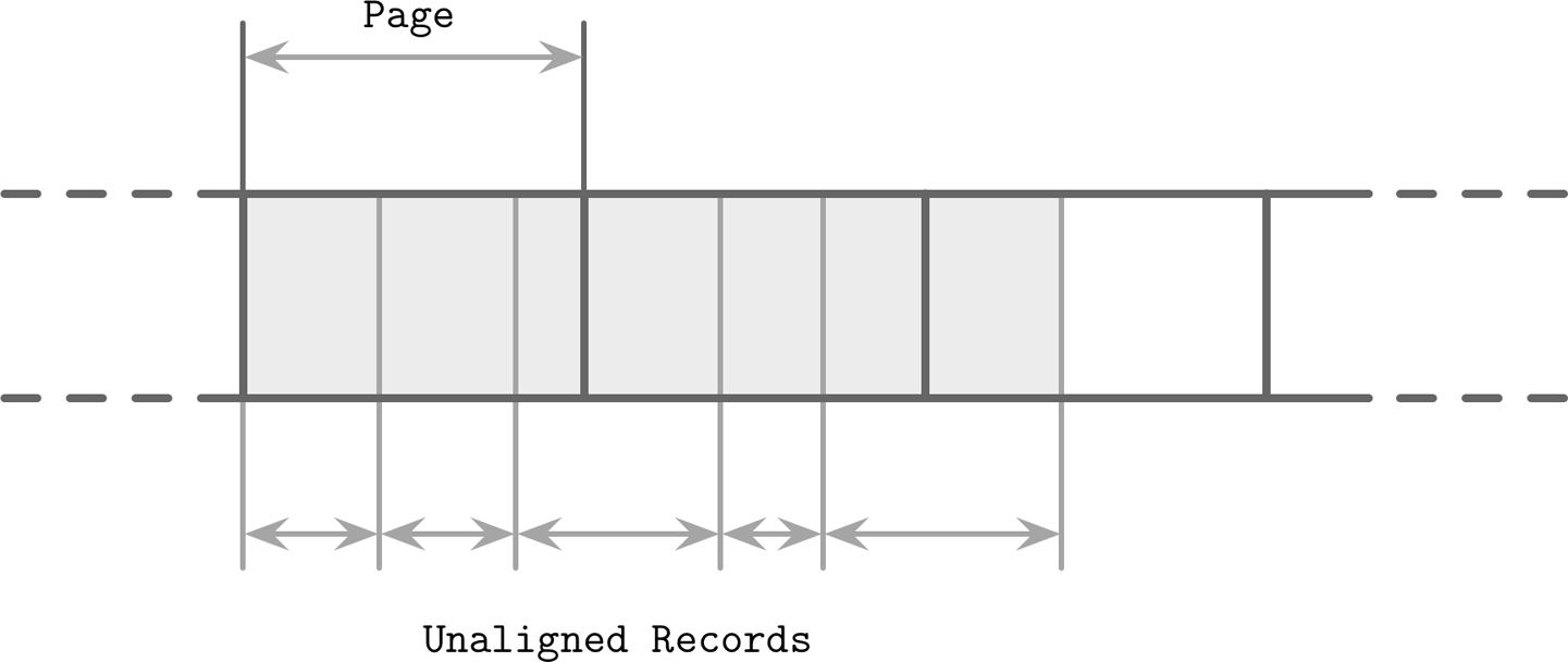
Figure 7-9. Unaligned data records

Compression

We’ve discussed compression already in context of B-Trees (see “Compression”). Similar ideas are also applicable to LSM Trees. The main difference here is that LSM Tree tables are immutable, and are generally written in a single pass. When compressing data page-wise, compressed pages are not page aligned, as their sizes are smaller than that of uncompressed ones.

To be able to address compressed pages, we need to keep track of the address boundaries when writing their contents. We could fill compressed pages with zeros, aligning them to the page size, but then we’d lose the benefits of compression.

To make compressed pages addressable, we need an indirection layer which stores offsets and sizes of compressed pages. Figure 7-10 shows the mapping between compressed and uncompressed blocks. Compressed pages are always smaller than the originals, since otherwise there’s no point in compressing them.

Figure 7-10. Reading compressed blocks. Dotted lines represent pointers from the mapping table to the offsets of compressed pages on disk. Uncompressed pages generally reside in the page cache.

During compaction and flush, compressed pages are appended sequentially, and compression information (the original uncompressed page offset and the actual compressed page offset) is stored in a separate file segment. During the read, the compressed page offset and its size are looked up, and the page can be uncompressed and materialized in memory.

Bitcask

Bitcask, one of the storage engines used in Riak, is an unordered log-structured storage engine [SHEEHY10b]. Unlike the log-structured storage implementations discussed so far, it does not use memtables for buffering, and stores data records directly in logfiles.

To make values searchable, Bitcask uses a data structure called keydir, which holds references to the latest data records for the corresponding keys. Old data records may still be present on disk, but are not referenced from keydir, and are garbage-collected during compaction. Keydir is implemented as an in-memory hashmap and has to be rebuilt from the logfiles during startup.

During a write, a key and a data record are appended to the logfile sequentially, and the pointer to the newly written data record location is placed in keydir.

Reads check the keydir to locate the searched key and follow the associated pointer to the logfile, locating the data record. Since at any given moment there can be only one value associated with the key in the keydir, point queries do not have to merge data from multiple sources.

Figure 7-11 shows mapping between the keys and records in data files in Bitcask. Logfiles hold data records, and keydir points to the latest live data record associated with each key. Shadowed records in data files (ones that were superseded by later writes or deletes) are shown in gray.

Figure 7-11. Mapping between keydir and data files in Bitcask. Solid lines represent pointers from the key to the latest value associated with it. Shadowed key/value pairs are shown in light gray.

During compaction, contents of all logfiles are read sequentially, merged, and written to a new location, preserving only live data records and discarding the shadowed ones. Keydir is updated with new pointers to relocated data records.

Data records are stored directly in logfiles, so a separate write-ahead log doesn’t have to be maintained, which reduces both space overhead and write amplification. A downside of this approach is that it offers only point queries and doesn’t allow range scans, since items are unordered both in keydir and in data files.

Advantages of this approach are simplicity and great point query performance. Even though multiple versions of data records exist, only the latest one is addressed by keydir. However, having to keep all keys in memory and rebuilding keydir on startup are limitations that might be a deal breaker for some use cases. While this approach is great for point queries, it does not offer any support for range queries.

WiscKey

Range queries are important for many applications, and it would be great to have a storage structure that could have the write and space advantages of unordered storage, while still allowing us to perform range scans.

WiscKey [LU16] decouples sorting from garbage collection by keeping the keys sorted in LSM Trees, and keeping data records in unordered append-only files called vLogs (value logs). This approach can solve two problems mentioned while discussing Bitcask: a need to keep all keys in memory and to rebuild a hashtable on startup.

Figure 7-12 shows key components of WiscKey, and mapping between keys and log files. vLog files hold unordered data records. Keys are stored in sorted LSM Trees, pointing to the latest data records in the logfiles.

Since keys are typically much smaller than the data records associated with them, compacting them is significantly more efficient. This approach can be particularly useful for use cases with a low rate of updates and deletes, where garbage collection won’t free up as much disk space.

The main challenge here is that because vLog data is unsorted, range scans require random I/O. WiscKey uses internal SSD parallelism to prefetch blocks in parallel during range scans and reduce random I/O costs. In terms of block transfers, the costs are still high: to fetch a single data record during the range scan, the entire page where it is located has to be read.

Figure 7-12. Key components of WiscKey: index LSM Trees and vLog files, and relationships between them. Shadowed records in data files (ones that were superseded by later writes or deletes) are shown in gray. Solid lines represent pointers from the key in the LSM tree to the latest value in the log file.

During compaction, vLog file contents are read sequentially, merged, and written to a new location. Pointers (values in a key LSM Tree) are updated to point to these new locations. To avoid scanning entire vLog contents, WiscKey uses head and tail pointers, holding information about vLog segments that hold live keys.

Since data in vLog is unsorted and contains no liveness information, the key tree has to be scanned to find which values are still live. Performing these checks during garbage collection introduces additional complexity: traditional LSM Trees can resolve file contents during compaction without addressing the key index.

Flash Translation Layer

Using a log-structuring mapping layer in SSDs is motivated by two factors: small random writes have to be batched together in a physical page, and the fact that SSDs work by using program/erase cycles. Writes can be done only into previously erased pages. This means that a page cannot be programmed (in other words, written) unless it is empty (in other words, was erased).

A single page cannot be erased, and only groups of pages in a block (typically holding 64 to 512 pages) can be erased together. Figure 7-13 shows a schematic representation of pages, grouped into blocks. The flash translation layer (FTL) translates logical page addresses to their physical locations and keeps track of page states (live, discarded, or empty). When FTL runs out of free pages, it has to perform garbage collection and erase discarded pages.

Figure 7-13. SSD pages, grouped into blocks

There are no guarantees that all pages in the block that is about to be erased are discarded. Before the block can be erased, FTL has to relocate its live pages to one of the blocks containing empty pages. Figure 7-14 shows the process of moving live pages from one block to new locations.

Figure 7-14. Page relocation during garbage collection

When all live pages are relocated, the block can be safely erased, and its empty pages become available for writes. Since FTL is aware of page states and state transitions and has all the necessary information, it is also responsible for SSD wear leveling.

In summary, the motivation for using log-structured storage on SSDs is to amortize I/O costs by batching small random writes together, which generally results in a smaller number of operations and, subsequently, reduces the number of times the garbage collection is triggered.

Filesystem Logging

On top of that, we get filesystems, many of which also use logging techniques for write buffering to reduce write amplification and use the underlying hardware optimally.

Log stacking manifests in a few different ways. First, each layer has to perform its own bookkeeping, and most often the underlying log does not expose the information necessary to avoid duplicating the efforts.

Figure 7-15 shows a mapping between a higher-level log (for example, the application) and a lower-level log (for example, the filesystem) resulting in redundant logging and different garbage collection patterns [YANG14]. Misaligned segment writes can make the situation even worse, since discarding a higher-level log segment may cause fragmentation and relocation of the neighboring segments’ parts.

Figure 7-15. Misaligned writes and discarding of a higher-level log segment

Because layers do not communicate LSS-related scheduling (for example, discarding or relocating segments), lower-level subsystems might perform redundant operations on discarded data or the data that is about to be discarded. Similarly, because there’s no single, standard segment size, it may happen that unaligned higher-level segments occupy multiple lower-level segments. All these overheads can be reduced or completely avoided.

Even though we say that log-structured storage is all about sequential I/O, we have to keep in mind that database systems may have multiple write streams (for example, log writes parallel to data record writes) [YANG14]. When considered on a hardware level, interleaved sequential write streams may not translate into the same sequential pattern: blocks are not necessarily going to be placed in write order. Figure 7-16 shows multiple streams overlapping in time, writing records that have sizes not aligned with the underlying hardware page size.

Figure 7-16. Unaligned multistream writes

This results in fragmentation that we tried to avoid. To reduce interleaving, some database vendors recommend keeping the log on a separate device to isolate workloads and be able to reason about their performance and access patterns independently. However, it is more important to keep partitions aligned to the underlying hardware [INTEL14] and keep writes aligned to page size [KIM12].

Open-Channel SSDs

An alternative to stacking software layers is to skip all indirection layers and use the hardware directly. For example, it is possible to avoid using a filesystem and flash translation layer by developing for Open-Channel SSDs. This way, we can avoid at least two layers of logs and have more control over wear-leveling, garbage collection, data placement, and scheduling. One of the implementations that uses this approach is LOCS (LSM Tree-based KV Store on Open-Channel SSD) [ZHANG13]. Another example using Open-Channel SSDs is LightNVM, implemented in the Linux kernel [BJØRLING17].

The flash translation layer usually handles data placement, garbage collection, and page relocation. Open-Channel SSDs expose their internals, drive management, and I/O scheduling without needing to go through the FTL. While this certainly requires much more attention to detail from the developer’s perspective, this approach may yield significant performance improvements. You can draw a parallel with using the O_DIRECT flag to bypass the kernel page cache, which gives better control, but requires manual page management.

Software Defined Flash (SDF) [OUYANG14], a hardware/software codesigned Open-Channel SSDs system, exposes an asymmetric I/O interface that takes SSD specifics into consideration. Sizes of read and write units are different, and write unit size corresponds to erase unit size (block), which greatly reduces write amplification. This setting is ideal for log-structured storage, since there’s only one software layer that performs garbage collection and relocates pages. Additionally, developers have access to internal SSD parallelism, since every channel in SDF is exposed as a separate block device, which can be used to further improve performance.

Hiding complexity behind a simple API might sound compelling, but can cause complications in cases in which software layers have different semantics. Exposing some underlying system internals may be beneficial for better integration.