Solid State Drives

Solid state drives (SSDs) do not have moving parts: there’s no disk that spins, or head that has to be positioned for the read. A typical SSD is built of memory cells, connected into strings (typically 32 to 64 cells per string), strings are combined into arrays, arrays are combined into pages, and pages are combined into blocks [LARRIVEE15].

Depending on the exact technology used, a cell can hold one or multiple bits of data. Pages vary in size between devices, but typically their sizes range from 2 to 16 Kb. Blocks typically contain 64 to 512 pages. Blocks are organized into planes and, finally, planes are placed on a die. SSDs can have one or more dies. Figure 2-5 shows this hierarchy.

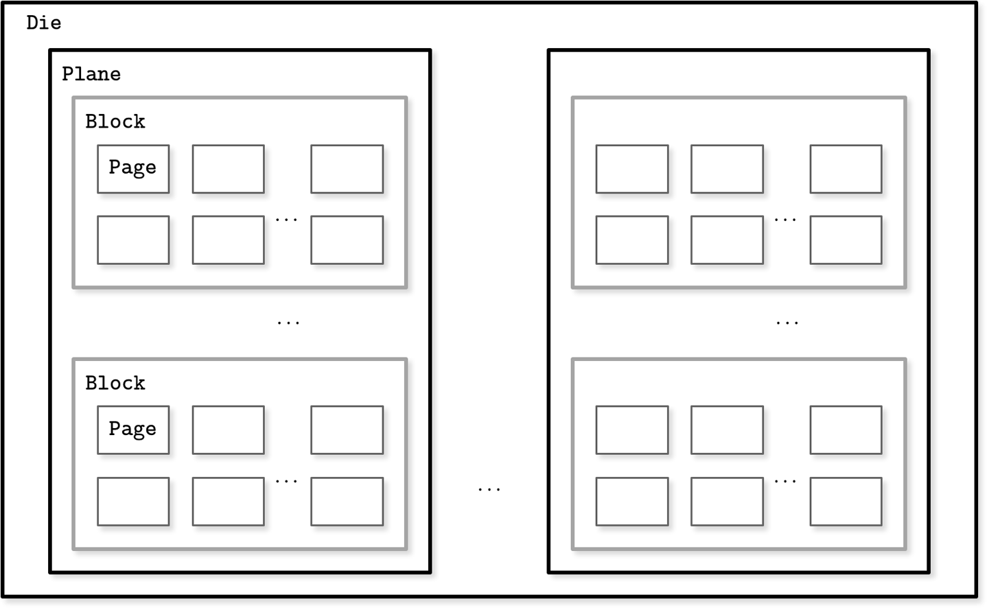
Figure 2-5. SSD organization schematics

The smallest unit that can be written (programmed) or read is a page. However, we can only make changes to the empty memory cells (i.e., to ones that have been erased before the write). The smallest erase entity is not a page, but a block that holds multiple pages, which is why it is often called an erase block. Pages in an empty block have to be written sequentially.

The part of a flash memory controller responsible for mapping page IDs to their physical locations, tracking empty, written, and discarded pages, is called the Flash Translation Layer (FTL) (see “Flash Translation Layer” for more about FTL). It is also responsible for garbage collection, during which FTL finds blocks it can safely erase. Some blocks might still contain live pages. In this case, it relocates live pages from these blocks to new locations and remaps page IDs to point there. After this, it erases the now-unused blocks, making them available for writes.

Since in both device types (HDDs and SSDs) we are addressing chunks of memory rather than individual bytes (i.e., accessing data block-wise), most operating systems have a block device abstraction [CESATI05]. It hides an internal disk structure and buffers I/O operations internally, so when we’re reading a single word from a block device, the whole block containing it is read. This is a constraint we cannot ignore and should always take into account when working with disk-resident data structures.

In SSDs, we don’t have a strong emphasis on random versus sequential I/O, as in HDDs, because the difference in latencies between random and sequential reads is not as large. There is still some difference caused by prefetching, reading contiguous pages, and internal parallelism [GOOSSAERT14].

Even though garbage collection is usually a background operation, its effects may negatively impact write performance, especially in cases of random and unaligned write workloads.

Writing only full blocks, and combining subsequent writes to the same block, can help to reduce the number of required I/O operations. We discuss buffering and immutability as ways to achieve that in later chapters.

On-Disk Structures

Besides the cost of disk access itself, the main limitation and design condition for building efficient on-disk structures is the fact that the smallest unit of disk operation is a block. To follow a pointer to the specific location within the block, we have to fetch an entire block. Since we already have to do that, we can change the layout of the data structure to take advantage of it.

We’ve mentioned pointers several times throughout this chapter already, but this word has slightly different semantics for on-disk structures. On disk, most of the time we manage the data layout manually (unless, for example, we’re using memory mapped files). This is still similar to regular pointer operations, but we have to compute the target pointer addresses and follow the pointers explicitly.

Most of the time, on-disk offsets are precomputed (in cases when the pointer is written on disk before the part it points to) or cached in memory until they are flushed on the disk. Creating long dependency chains in on-disk structures greatly increases code and structure complexity, so it is preferred to keep the number of pointers and their spans to a minimum.

In summary, on-disk structures are designed with their target storage specifics in mind and generally optimize for fewer disk accesses. We can do this by improving locality, optimizing the internal representation of the structure, and reducing the number of out-of-page pointers.

In “Binary Search Trees”, we came to the conclusion that high fanout and low height are desired properties for an optimal on-disk data structure. We’ve also just discussed additional space overhead coming from pointers, and maintenance overhead from remapping these pointers as a result of balancing. B-Trees combine these ideas: increase node fanout, and reduce tree height, the number of node pointers, and the frequency of balancing operations.

B-Tree Hierarchy

B-Trees consist of multiple nodes. Each node holds up to N keys and N + 1 pointers to the child nodes. These nodes are logically grouped into three groups:

Root node

This has no parents and is the top of the tree.

Leaf nodes

These are the bottom layer nodes that have no child nodes.

Internal nodes

These are all other nodes, connecting root with leaves. There is usually more than one level of internal nodes.

This hierarchy is shown in Figure 2-9.

Figure 2-9. B-Tree node hierarchy

Since B-Trees are a page organization technique (i.e., they are used to organize and navigate fixed-size pages), we often use terms node and page interchangeably.

The relation between the node capacity and the number of keys it actually holds is called occupancy.

B-Trees are characterized by their fanout: the number of keys stored in each node. Higher fanout helps to amortize the cost of structural changes required to keep the tree balanced and to reduce the number of seeks by storing keys and pointers to child nodes in a single block or multiple consecutive blocks. Balancing operations (namely, splits and merges) are triggered when the nodes are full or nearly empty.

Separator Keys

Keys stored in B-Tree nodes are called index entries, separator keys, or divider cells. They split the tree into subtrees (also called branches or subranges), holding corresponding key ranges. Keys are stored in sorted order to allow binary search. A subtree is found by locating a key and following a corresponding pointer from the higher to the lower level.

The first pointer in the node points to the subtree holding items less than the first key, and the last pointer in the node points to the subtree holding items greater than or equal to the last key. Other pointers are reference subtrees between the two keys: Ki-1 ≤ Ks < Ki, where K is a set of keys, and Ks is a key that belongs to the subtree. Figure 2-10 shows these invariants.

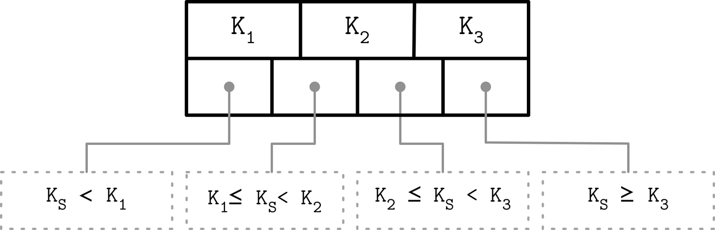
Figure 2-10. How separator keys split a tree into subtrees

Some B-Tree variants also have sibling node pointers, most often on the leaf level, to simplify range scans. These pointers help avoid going back to the parent to find the next sibling. Some implementations have pointers in both directions, forming a double-linked list on the leaf level, which makes the reverse iteration possible.

What sets B-Trees apart is that, rather than being built from top to bottom (as binary search trees), they’re constructed the other way around—from bottom to top. The number of leaf nodes grows, which increases the number of internal nodes and tree height.

Since B-Trees reserve extra space inside nodes for future insertions and updates, tree storage utilization can get as low as 50%, but is usually considerably higher. Higher occupancy does not influence B-Tree performance negatively.

B-Tree Lookup Complexity

B-Tree lookup complexity can be viewed from two standpoints: the number of block transfers and the number of comparisons done during the lookup.

In terms of number of transfers, the logarithm base is N (number of keys per node). There are N times more nodes on each new level, and following a child pointer reduces the search space by the factor of N. During lookup, at most logN M (where M is a total number of items in the B-Tree) pages are addressed to find a searched key. The number of child pointers that have to be followed on the root-to-leaf pass is also equal to the number of levels, in other words, the height h of the tree.

From the perspective of number of comparisons, the logarithm base is 2, since searching a key inside each node is done using binary search. Every comparison halves the search space, so complexity is log2 M.

Knowing the distinction between the number of seeks and the number of comparisons helps us gain the intuition about how searches are performed and understand what lookup complexity is, from both perspectives.

In textbooks and articles,² B-Tree lookup complexity is generally referenced as log M. Logarithm base is generally not used in complexity analysis, since changing the base simply adds a constant factor, and multiplication by a constant factor does not change complexity. For example, given the nonzero constant factor c, O(|c| × n) == O(n) [KNUTH97].

B-Tree Lookup Algorithm

Now that we have covered the structure and internal organization of B-Trees, we can define algorithms for lookups, insertions, and removals. To find an item in a B-Tree, we have to perform a single traversal from root to leaf. The objective of this search is to find a searched key or its predecessor. Finding an exact match is used for point queries, updates, and deletions; finding its predecessor is useful for range scans and inserts.

The algorithm starts from the root and performs a binary search, comparing the searched key with the keys stored in the root node until it finds the first separator key that is greater than the searched value. This locates a searched subtree. As we’ve discussed previously, index keys split the tree into subtrees with boundaries between two neighboring keys. As soon as we find the subtree, we follow the pointer that corresponds to it and continue the same search process (locate the separator key, follow the pointer) until we reach a target leaf node, where we either find the searched key or conclude it is not present by locating its predecessor.

On each level, we get a more detailed view of the tree: we start on the most coarse-grained level (the root of the tree) and descend to the next level where keys represent more precise, detailed ranges, until we finally reach leaves, where the data records are located.

During the point query, the search is done after finding or failing to find the searched key. During the range scan, iteration starts from the closest found key-value pair and continues by following sibling pointers until the end of the range is reached or the range predicate is exhausted.

Counting Keys

Across the literature, you can find different ways to describe key and child offset counts. [BAYER72] mentions the device-dependent natural number k that represents an optimal page size. Pages, in this case, can hold between k and 2k keys, but can be partially filled and hold at least k + 1 and at most 2k + 1 pointers to child nodes. The root page can hold between 1 and 2k keys. Later, a number l is introduced, and it is said that any nonleaf page can have l + 1 keys.

Other sources, for example [GRAEFE11], describe nodes that can hold up to N separator keys and N + 1 pointers, with otherwise similar semantics and invariants.

Both approaches bring us to the same result, and differences are only used to emphasize the contents of each source. In this book, we stick to N as the number of keys (or key-value pairs, in the case of the leaf nodes) for clarity.

B-Tree Node Splits

To insert the value into a B-Tree, we first have to locate the target leaf and find the insertion point. For that, we use the algorithm described in the previous section. After the leaf is located, the key and value are appended to it. Updates in B-Trees work by locating a target leaf node using a lookup algorithm and associating a new value with an existing key.

If the target node doesn’t have enough room available, we say that the node has overflowed [NICHOLS66] and has to be split in two to fit the new data. More precisely, the node is split if the following conditions hold:

• For leaf nodes: if the node can hold up to N key-value pairs, and inserting one more key-value pair brings it over its maximum capacity N.

• For nonleaf nodes: if the node can hold up to N + 1 pointers, and inserting one more pointer brings it over its maximum capacity N + 1.

Splits are done by allocating the new node, transferring half the elements from the splitting node to it, and adding its first key and pointer to the parent node. In this case, we say that the key is promoted. The index at which the split is performed is called the split point (also called the midpoint). All elements after the split point (including split point in the case of nonleaf node split) are transferred to the newly created sibling node, and the rest of the elements remain in the splitting node.

If the parent node is full and does not have space available for the promoted key and pointer to the newly created node, it has to be split as well. This operation might propagate recursively all the way to the root.

As soon as the tree reaches its capacity (i.e., split propagates all the way up to the root), we have to split the root node. When the root node is split, a new root, holding a split point key, is allocated. The old root (now holding only half the entries) is demoted to the next level along with its newly created sibling, increasing the tree height by one. The tree height changes when the root node is split and the new root is allocated, or when two nodes are merged to form a new root. On the leaf and internal node levels, the tree only grows horizontally.

Figure 2-11 shows a fully occupied leaf node during insertion of the new element 11. We draw the line in the middle of the full node, leave half the elements in the node, and move the rest of elements to the new one. A split point value is placed into the parent node to serve as a separator key.

Figure 2-11. Leaf node split during the insertion of 11. New element and promoted key are shown in gray.

Figure 2-12 shows the split process of a fully occupied nonleaf (i.e., root or internal) node during insertion of the new element 11. To perform a split, we first create a new node and move elements starting from index N/2 + 1 to it. The split point key is promoted to the parent.

Figure 2-12. Nonleaf node split during the insertion of 11. New element and promoted key are shown in gray.

Since nonleaf node splits are always a manifestation of splits propagating from the levels below, we have an additional pointer (to the newly created node on the next level). If the parent does not have enough space, it has to be split as well.

It doesn’t matter whether the leaf or nonleaf node is split (i.e., whether the node holds keys and values or just the keys). In the case of leaf split, keys are moved together with their associated values.

When the split is done, we have two nodes and have to pick the correct one to finish insertion. For that, we can use the separator key invariants. If the inserted key is less than the promoted one, we finish the operation by inserting to the split node. Otherwise, we insert to the newly created one.

To summarize, node splits are done in four steps:

1. Allocate a new node.

2. Copy half the elements from the splitting node to the new one.

3. Place the new element into the corresponding node.

4. At the parent of the split node, add a separator key and a pointer to the new node.

B-Tree Node Merges

Deletions are done by first locating the target leaf. When the leaf is located, the key and the value associated with it are removed.

If neighboring nodes have too few values (i.e., their occupancy falls under a threshold), the sibling nodes are merged. This situation is called underflow. [BAYER72] describes two underflow scenarios: if two adjacent nodes have a common parent and their contents fit into a single node, their contents should be merged (concatenated); if their contents do not fit into a single node, keys are redistributed between them to restore balance (see “Rebalancing”). More precisely, two nodes are merged if the following conditions hold:

• For leaf nodes: if a node can hold up to N key-value pairs, and a combined number of key-value pairs in two neighboring nodes is less than or equal to N.

• For nonleaf nodes: if a node can hold up to N + 1 pointers, and a combined number of pointers in two neighboring nodes is less than or equal to N + 1.

Figure 2-13 shows the merge during deletion of element 16. To do this, we move elements from one of the siblings to the other one. Generally, elements from the right sibling are moved to the left one, but it can be done the other way around as long as the key order is preserved.

Figure 2-13. Leaf node merge

Figure 2-14 shows two sibling nonleaf nodes that have to be merged during deletion of element 10. If we combine their elements, they fit into one node, so we can have one node instead of two. During the merge of nonleaf nodes, we have to pull the corresponding separator key from the parent (i.e., demote it). The number of pointers is reduced by one because the merge is a result of the propagation of the pointer deletion from the lower level, caused by the page removal. Just as with splits, merges can propagate all the way to the root level.

Figure 2-14. Nonleaf node merge

To summarize, node merges are done in three steps, assuming the element is already removed:

1. Copy all elements from the right node to the left one.

2. Remove the right node pointer from the parent (or demote it in the case of a nonleaf merge).

3. Remove the right node.

One of the techniques often implemented in B-Trees to reduce the number of splits and merges is rebalancing, which we discuss in “Rebalancing”.