12.4 Data Placement
One of the most important decisions a distributed database designer must make is data placement. Proper data placement is a crucial factor in determining the success of a DDBS. There are four basic alternatives, namely, centralized, replicated, partitioned, and hybrid. Some of these require additional analysis to fine-tune the placement of data. In deciding among data placement alternatives, the following factors need to be considered:
Locality of data reference. The data should be placed at the site where it is used most often. The designer studies the applications to identify the sites where they are performed and attempts to place the data in such a way that most accesses are local.
Reliability of the data. By storing multiple copies of the data in geographically remote sites, the designer maximizes the probability that the data will be recoverable in case of physical damage to any site.
Data availability. As with reliability, storing multiple copies assures users that data items will be available to them, even if the site from which the items are normally accessed is unavailable due to failure of the node or its only link.
Storage capacities and costs. Nodes can have different storage capacities and storage costs that must be considered in deciding where data should be kept. Storage costs are minimized when a single copy of each data item is kept, but the plunging costs of data storage make this consideration less important.
Distribution of processing load. One of the reasons for choosing a distributed system is to distribute the workload so that processing power will be used most effectively. This objective must be balanced against locality of data reference.
Communications costs. The designer must consider the cost of using the communications network to retrieve data. Retrieval costs and retrieval time are minimized when each site has its own copy of all the data. However, when the data is updated, the changes must then be sent to all sites. If the data is very volatile, this results in high communications costs for update synchronization.
The four placement alternatives, as shown in FIGURE 12.6, are the following:
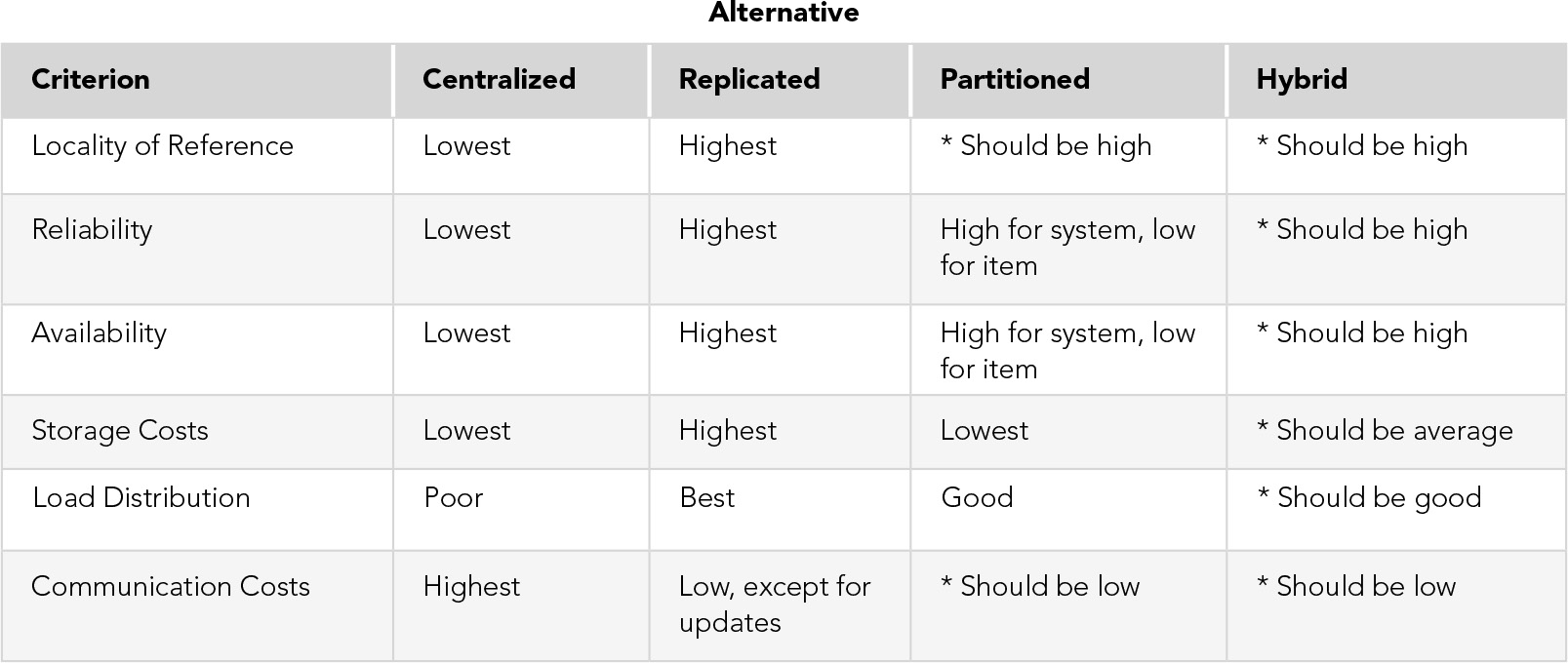
FIGURE 12.6 Evaluation of Data Placement Alternatives
*Depends on exact data placement decision made
Centralized. This alternative consists of a single database and DBMS stored in one location, with users distributed, as illustrated in Figure 12.1. There is no need for a DDBMS or global data dictionary because there is no real distribution of data, only of processing. Retrieval costs are high because all users, except those at the central site, use the network for all accesses. Storage costs are low because only one copy of each item is kept. There is no need for update synchronization, and the standard concurrency control mechanism is sufficient. Reliability is low and availability is poor because a failure at the central node results in the loss of the entire system. The workload can be distributed, but remote nodes need to access the database to perform applications, so locality of data reference is low. This alternative is not a true DDBS.
Replicated. With this alternative, a complete copy of the database is kept at each node. Advantages are maximum locality of reference, reliability, data availability, and processing load distribution. Storage costs are highest in this alternative. Communications costs for retrievals are low, but the cost of updates is high because every site must receive every update. If updates are very infrequent, this alternative is a good one.
Partitioned. Here, there is only one copy of each data item, but the data is distributed across nodes. To allow this, the database is split into disjoint fragments or parts. If the database is a relational one, fragments can be vertical table subsets (formed by projection) or horizontal subsets (formed by selection) of global relations. FIGURE 12.7 provides examples of fragmentation. In any horizontal fragmentation scheme, each tuple of every relation must be assigned to one or more fragments such that taking the union of the fragments results in the original relation; for the horizontally partitioned case, a tuple is assigned to exactly one fragment. In a vertical fragmentation scheme, the projections must be lossless, so that the original relations can be reconstructed by taking the join of the fragments. The easiest method of ensuring that projections are lossless is, of course, to include the key in each fragment; however, this violates the disjointness condition because key attributes would then be replicated. The designer can choose to accept key replication, or the system can add a tuple ID—a unique identifier for each tuple—invisible to the user. The system would then include the tuple ID in each vertical fragment of the tuple and would use that identifier to perform joins.
Besides vertical and horizontal fragments, there can be mixed fragments, obtained by successive applications of select and project operations. Partitioning requires careful analysis to ensure that data items are assigned to the appropriate site. If data items have been assigned to the site where they are used most often, locality of data reference will be high with this alternative. Because only one copy of each item is stored, data reliability and availability for a specific item are low. However, failure of a node results in the loss of only that node’s data, so the systemwide reliability and availability are higher than in the centralized case. Storage costs are low, and the communications costs of a well-designed system should be low. The processing load should also be well distributed if the data is properly distributed.
Hybrid. In this alternative different portions of the database are distributed differently. For example, those records with high locality of reference are partitioned, while those commonly used by all nodes are replicated, if updates are infrequent. Those that are needed by all nodes but updated so frequently that synchronization would be a problem, might be centralized. This alternative is designed to optimize data placement, so that all the advantages and none of the disadvantages of the other methods are possible. However, very careful analysis of data and processing is required with this plan.
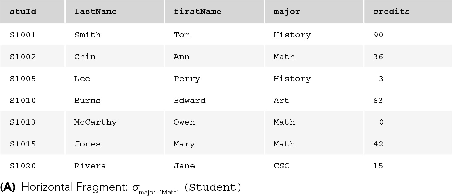
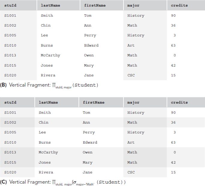
FIGURE 12.7 Fragmentation
As an example, let us consider how the University database schema might be distributed. We assume that the university has a main campus and four branch campuses (North, South, East, and West), and that students have a home campus where they normally register and take classes. However, students can register for any class at any campus. Faculty members teach at a single campus. Each class is offered at a single campus. We will modify the schema slightly to include campus information in our new global schema:

It is reasonable to assume that Student records are used most often at the student’s home campus, so we would partition the Student relation, placing each student’s record at his or her home campus. The same is true for Faculty records. The Class relation could also be partitioned according to the campus where the class is offered. However, this would mean that queries about offerings at other campuses would always require use of the network. If such queries are frequent, an alternative would be to replicate the entire Class relation at all sites. Because updates to this table are relatively infrequent, and most accesses are read-only, replication would reduce communication costs, so we will choose this alternative. The Enroll table would not be a good candidate for replication because during registration, updates must be done quickly, and updating multiple copies is time-consuming. It is desirable to have the Enroll records at the same site as the Student record and as the Class record, but these may not be the same site. Therefore, we might choose to centralize the Enroll records at the main site, possibly with copies at the Student site and the Class site. We can designate the main site as the primary copy for Enroll. The fragmentation scheme would be expressed by specifying the conditions for selecting records, as in
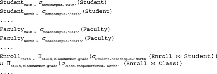
We are not fragmenting the Class relation. Because we have made different decisions for different parts of the database, this is a hybrid fragmentation scheme. FIGURE 12.8 illustrates the data placement decisions for this example.
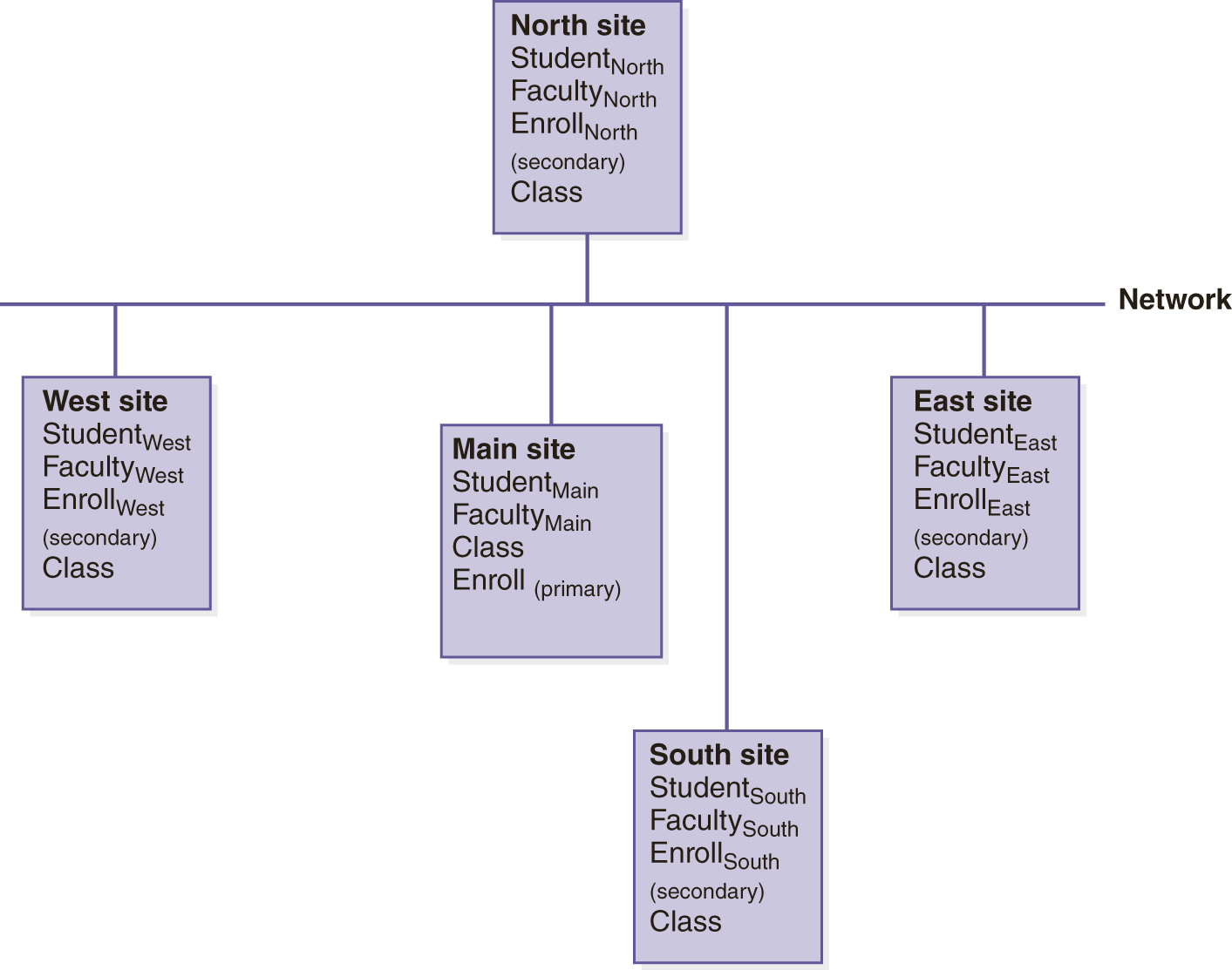
FIGURE 12.8 Data Placement for the Distributed University Schema