8. Training Deep Networks
In the preceding chapters, we described artificial neurons comprehensively and we walked through the process of forward propagating information through a network of neurons to output a prediction, such as whether a given fast food item is a hot dog, a juicy burger, or a greasy slice of pizza. In those culinary examples from Chapters 6 and 7, we fabricated numbers for the neuron parameters—the neuron weights and biases. In real-world applications, however, these parameters are not typically concocted arbitrarily: They are learned by training the network on data.
In this chapter, you will become acquainted with two techniques—called gradient descent and backpropagation—that work in tandem to learn artificial neural network parameters. As usual in this book, our presentation of these methods is not only theoretical: We provide pragmatic best practices for implementing the techniques. The chapter culminates in the application of these practices to the construction of a neural network with more than one hidden layer.
Cost Functions
In Chapter 7, you discovered that, upon forward propagating some input values all the way through an artificial neural network, the network provides its estimated output, which is denoted ŷ. If a network were perfectly calibrated, it would output ŷ values that are exactly equal to the true label y. In our binary classifier for detecting hot dogs, for example (Figure 7.3), y = 1 indicated that the object presented to the network is a hot dog, while y = 0 indicated that it’s something else. In an instance where we have in fact presented a hot dog to the network, therefore, ideally it would output ŷ = 1.
In practice, the gold standard of ŷ = y is not always attained and so may be an excessively stringent definition of the “correct” ŷ. Instead, if y = 1 we might be quite pleased to see a ŷ of, say, 0.9997, because that would indicate that the network has an extremely high confidence that the object is a hot dog. A ŷ of 0.9 might be considered acceptable, ŷ = 0.6 to be disappointing, and ŷ = 0.1192 (as computed in Equation 7.7) to be awful.
To quantify the spectrum of output-evaluation sentiments from “quite pleased” all the way down to “awful,” machine learning algorithms often involve cost functions (also known as loss functions). The two such functions that we cover in this book are called quadratic cost and cross-entropy cost. Let’s cover them in turn.
Quadratic Cost
Quadratic cost is one of the simplest cost functions to calculate. It is alternatively called mean squared error, which handily describes all that there is to its calculation:
For any given instance i, we calculate the difference (the error) between the true label yi and the network’s estimated ŷi. We then square this difference, for two reasons:
Squaring ensures that whether y is greater than ŷ or vice versa, the difference between the two is stated as a positive value.
Squaring penalizes large differences between y and ŷ much more severely than small differences.
Having obtained a squared error for each instance i by using (yi − ŷi)2, we can then calculate the mean cost C across all n of our instances by:
Summing up cost across all instances using
Dividing by however many instances we have using
By taking a peek inside the Quadratic Cost Jupyter notebook from the book’s GitHub repo, you can play around with Equation 8.1 yourself. At the top of the notebook, we define a function to calculate the squared error for an instance i:
def squared_error(y, yhat):
    return (y - yhat)**2
By plugging a true y of 1 and the ideal yhat of 1 in to the function by using squared_error(1, 1), we observe that—as desired—this perfect estimate is associated with a cost of 0. Likewise, minor deviations from the ideal, such as a yhat of 0.9997, correspond to an extremely small cost: 9.0e-08.1 As the difference between y and yhat increases, we witness the expected exponential increase in cost: Holding y steady at 1 but lowering yhat from 0.9 to 0.6, and then to 0.1192, the cost climbs increasingly rapidly from 0.01 to 0.16 and then to 0.78. As a final bit of amusement in the notebook, we note that had y truly been 0, our yhat of 0.1192 would be associated with a small cost: 0.0142.
1. 9.0e-08 is equivalent to 9.0 × 10⁻⁸.
Saturated Neurons
While quadratic cost serves as a straightforward introduction to loss functions, it has a vital flaw. Consider Figure 8.1, in which we recapitulate the tanh activation function from Figure 6.10. The issue presented in the figure, called neuron saturation, is common across all activation functions, but we’ll use tanh as our lone exemplar. A neuron is considered saturated when the combination of its inputs and parameters (interacting as per “the most important equation,” z = w · x + b, which is captured in Figure 6.10) produces extreme values of z—the areas encircled with red in the plot in Figure 8.1. In these areas, changes in z (via adjustments to the neuron’s underlying parameters w and b) cause only teensy-weensy changes in the neuron’s activation a.2
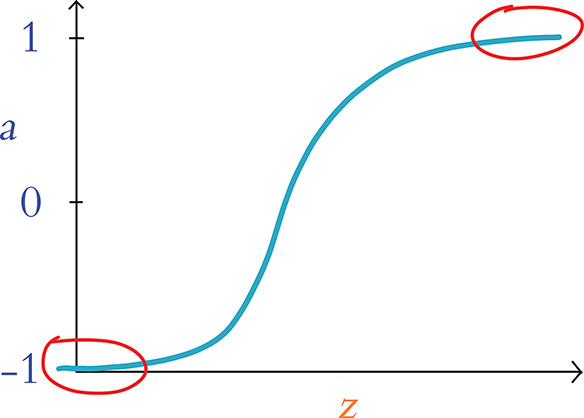
Figure 8.1 Plot reproducing the tanh activation function shown in Figure 6.10, drawing attention to the high and low values of z at which a neuron is saturated
2. Recall from Chapter 6 that a = σ( z), where σ is some activation function—in this example, the tanh function.
Using methods that we cover later in this chapter—namely, gradient descent and backpropagation—a neural network is able to learn to approximate y through the tuning of the parameters w and b associated with all of its constituent neurons. In a saturated neuron, where changes to w and b lead to only minuscule changes in a, this learning slows to a crawl: If adjustments to w and b make no discernible impact on a given neuron’s activation a, then these adjustments cannot have any discernible impact downstream (via forward propagation) on the network’s ŷ, its estimate of y.
Cross-Entropy Cost
One of the ways3 to minimize the impact of saturated neurons on learning speed is to use cross-entropy cost in lieu of quadratic cost. This alternative loss function is configured to enable efficient learning anywhere within the activation function curve of Figure 8.1. Because of this, it is a far more popular choice of cost function and it is the selection that predominates the remainder of this book.4
3. More methods for attenuating saturated neurons and their negative effects on a network are covered in Chapter 9.
4. Cross-entropy cost is well suited to neural networks solving classification problems, and such problems dominate this book. For regression problems (covered in Chapter 9), quadratic cost is a better option than cross-entropy cost.
You need not preoccupy yourself with the equation for cross-entropy cost, but for the sake of completeness, here it is:
The most pertinent aspects of the equation are:
Like quadratic cost, divergence of ŷ from y corresponds to increased cost.
Analogous to the use of the square in quadratic cost, the use of the natural logarithm ln in cross-entropy cost causes larger differences between ŷ and y to be associated with exponentially larger cost.
Cross-entropy cost is structured so that the larger the difference between ŷ and y, the faster the neuron is able to learn.5

5. To understand how the cross-entropy cost function in Equation 8.2 enables a neuron with larger cost to learn more rapidly, we require a touch of partial-derivative calculus. (Because we endeavor to minimize the use of advanced mathematics in this book, we’ve relegated this calculus-focused explanation to this footnote.) Central to the two computational methods that enable neural networks to learn—gradient descent and backpropagation—is the comparison of the rate of change of cost C relative to neuron parameters like weight w. Using partial-derivative notation, we can represent these relative rates of change as . The cross-entropy cost function is deliberately structured so that, when we calculate its derivative, is related to ( ŷ – y). Thus, the larger the difference between the ideal output y and the neuron’s estimated output ŷ, the greater the rate of change of cost C with respect to weight w.
To make it easier to remember that the greater the cost, the more quickly a neural network incorporating cross-entropy cost learns, here’s an analogy that would absolutely never involve any of your esteemed authors: Let’s say you’re at a cocktail party leading the conversation of a group of people that you’ve met that evening. The strong martini you’re holding has already gone to your head, and you go out on a limb by throwing a risqué line into your otherwise charming repartee. Your audience reacts with immediate, visible disgust. With this response clearly indicating that your quip was well off the mark, you learn pretty darn quickly. It’s exceedingly unlikely you’ll be repeating the joke anytime soon.
Anyway, that’s plenty enough on disasters of social etiquette. The final item to note on cross-entropy cost is that, by including ŷ, the formula provided in Equation 8.2 applies to only the output layer. Recall from Chapter 7 (specifically the discussion of Figure 7.3) that ŷ is a special case of a: It’s actually just another plain old a value—except that it’s being calculated by neurons in the output layer of a neural network. With this in mind, Equation 8.2 could be expressed with ai substituted in for ŷi so that the equation generalizes neatly beyond the output layer to neurons in any layer of a network:
To cement all of this theoretical chatter about cross-entropy cost, let’s interactively explore our aptly named Cross Entropy Cost Jupyter notebook. There is only one dependency in the notebook: the log function from the NumPy package, which enables us to compute the natural logarithm ln shown twice in Equation 8.3. We load this dependency using from numpy import log.
Next, we define a function for calculating cross-entropy cost for an instance i:
def cross_entropy(y, a):
     return -1*(y*log(a) + (1-y)*log (1-a))
Plugging the same values in to our cross_entropy() function as we did the squared_ error() function earlier in this chapter, we observe comparable behavior. As shown in Table 8.1, by holding y steady at 1 and gradually decreasing a from the nearly ideal estimate of 0.9997 downward, we get exponential increases in cross-entropy cost. The table further illustrates that—again, consistent with the behavior of its quadratic cousin—cross-entropy cost would be low, with an a of 0.1192, if y happened to in fact be 0. These results reiterate for us that the chief distinction between the quadratic and cross-entropy functions is not the particular cost value that they calculate per se, but rather it is the rate at which they learn within a neural net—especially if saturated neurons are involved.
Table 8.1 Cross-entropy costs associated with selected example inputs
y |
a |
C |
|---|---|---|
1 |
0.9997 |
0.0003 |
1 |
0.9 |
0.1 |
1 |
0.6 |
0.5 |
1 |
0.1192 |
2.1 |
0 |
0.1192 |
0.1269 |
1 |
1− 0.1192 |
0.1269 |
Optimization: Learning to Minimize Cost
Cost functions provide us with a quantification of how incorrect our model’s estimate of the ideal y is. This is most helpful because it arms us with a metric we can leverage to reduce our network’s incorrectness.
As alluded to a couple of times in this chapter, the primary approach for minimizing cost in deep learning paradigms is to pair an approach called gradient descent with another one called backpropagation. These approaches are optimizers and they enable the network to learn. This learning is accomplished by adjusting the model’s parameters so that its estimated ŷ gradually converges toward the target of y, and thus the cost decreases. We cover gradient descent first and move on to backpropagation immediately afterward.
Gradient Descent
Gradient descent is a handy, efficient tool for adjusting a model’s parameters with the aim of minimizing cost, particularly if you have a lot of training data available. It is widely used across the field of machine learning, not only in deep learning.
In Figure 8.2, we use a nimble trilobite in a cartoon to illustrate how gradient descent works. Along the horizontal axis in each frame is some parameter that we’ve denoted as p. In an artificial neural network, this parameter would be either a neuron’s weight w or bias b. In the top frame, the trilobite finds itself on a hill. Its goal is to descend the gradient, thereby finding the location with the minimum cost, C. But there’s a twist: The trilobite is blind! It cannot see whether deeper valleys lie far away somewhere, and so it can only use its cane to investigate the slope of the terrain in its immediate vicinity.
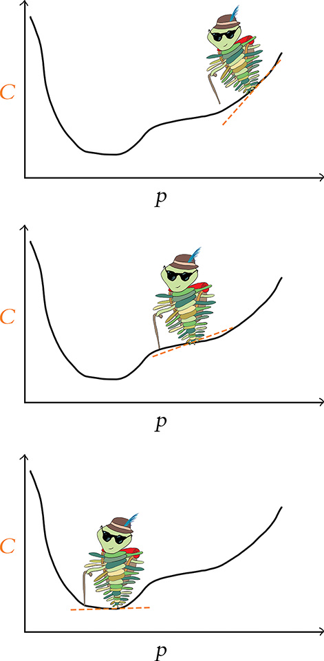
Figure 8.2 A trilobite using gradient descent to find the value of a parameter p associated with minimal cost, C
The dashed orange line in Figure 8.2 indicates the blind trilobite’s calculation of the slope at the point where it finds itself. According to that slope line, if the trilobite takes a step to the left (i.e., to a slightly lower value of p), it would be moving to a location with smaller cost. On the hand, if the trilobite takes a step to the right (a slightly higher value of p), it would be moving to a location with higher cost. Given the trilobite’s desire to descend the gradient, it chooses to take a step to the left.
By the middle frame, the trilobite has taken several steps to the left. Here again, we see it evaluating the slope with the orange line and discovering that, yet again, a step to the left will bring it to a location with lower cost, and so it takes another step left. In the lower frame, the trilobite has succeeded in making its way to the location—the value of the parameter p—corresponding to the minimum cost. From this position, if it were to take a step to the left or to the right, cost would go up, so it gleefully remains in place.
In practice, a deep learning model would not have only one parameter. It is not uncommon for deep learning networks to have millions of parameters, and some industrial applications have billions of them. Even our Shallow Net in Keras—one of the smallest models we build in this book—has 50,890 parameters (see Figure 7.5).
Although it’s impossible for the human mind to imagine a billion-dimensional space, the two-parameter cartoon shown in Figure 8.3 provides a sense of how gradient descent scales up to minimize cost across multiple parameters simultaneously. Across however many trainable parameters there are in a model, gradient descent iteratively evaluates slopes6 to identify the adjustments to those parameters that correspond to the steepest reduction in cost. With two parameters, as in the trilobite cartoon in Figure 8.3, for example, this procedure can be likened to a blind hike through the mountains, where:
Latitude represents one parameter, say p1.
Longitude represents the other parameter, p2.
Altitude represents cost—the lower the altitude, the better!
6. Using partial-derivative calculus.
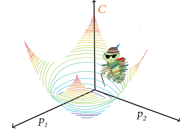
Figure 8.3 A trilobite exploring along two model parameters—p1 and p2—in order to minimize cost via gradient descent. In a mountain-adventure analogy, p1 and p2 could be thought of as latitude and longitude, and altitude represents cost.
The trilobite randomly finds itself at a location in the mountains. From that point, it feels around with its cane to identify the direction of the step it can take that will reduce its altitude the most. It then takes that single step. Repeating this process many times, the trilobite may eventually find itself at the latitude and longitude coordinates that correspond to the lowest-possible altitude (the minimum cost), at which point the trilobite’s surreal alpine adventure is complete.
Learning Rate
For conceptual simplicity, in Figure 8.4, let’s return to a blind trilobite navigating a single-parameter world instead of a two-parameter world. Now let’s imagine that we have a ray-gun that can shrink or enlarge trilobites. In the middle panel, we’ve used our ray-gun to make our trilobite very small. The trilobite’s steps will then be correspondingly small, and so it will take our intrepid little hiker a long time to find its way to the legendary valley of minimum cost. On the other hand, consider the bottom panel, in which we’ve used our ray-gun to make the trilobite very large. The situation here is even worse! The trilobite’s steps will now be so large that it will step right over the valley of minimum cost, and so it never has any hope of finding it.
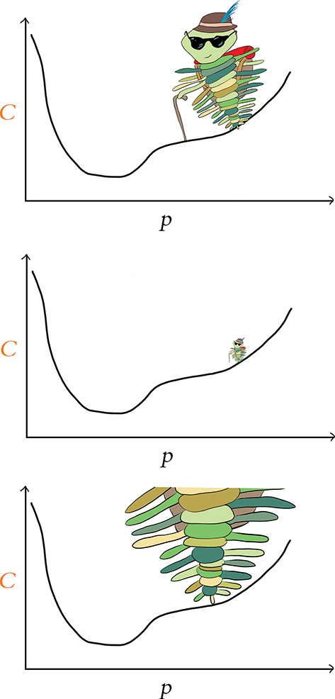
Figure 8.4 The learning rate (η) of gradient descent expressed as the size of a trilobite. The middle panel has a small learning rate, and the bottom panel, a large one.
In gradient descent terminology, step size is referred to as learning rate and denoted with the Greek letter η (eta, pronounced “ee-ta”). Learning rate is the first of several model hyperparameters that we cover in this book. In machine learning, including deep learning, hyperparameters are aspects of the model that we configure before we begin training the model. So hyperparameters such as η are preset while, in contrast, parameters—namely, w and b—are learned during training.
Getting your hyperparameters right for a given deep learning model often requires some trial and error. For the learning rate η, it’s something like the fairy tale of “Goldilocks and the Three Bears”: Too small and too large are both inadequate, but there’s a sweet spot in the middle. More specifically, as we portray in Figure 8.4, if η is too small, then it will take many, many iterations of gradient descent (read: an unnecessarily long time) to reach the minimal cost. On the other hand, selecting a value for η that is too large means we might never reach minimal cost at all: The gradient descent algorithm will act erratically as it jumps right over the parameters associated with minimal cost.
Coming up in Chapter 9, we have a clever trick waiting for you that will circumnavigate the need for you to manually select a given neural network’s η hyperparameter. In the interim, however, here are our rules of thumb on the topic:
Begin with a learning rate of about 0.01 or 0.001.
If your model is able to learn (i.e., if cost decreases consistently epoch over epoch) but training happens very slowly (i.e., each epoch, the cost decreases only a small amount), then increase your learning rate by an order of magnitude (e.g., from 0.01 to 0.1). If the cost begins to jump up and down erratically epoch over epoch, then you’ve gone too far, so rein in your learning rate.
At the other extreme, if your model is unable to learn, then your learning rate may be too high. Try decreasing it by orders of magnitude (e.g., from 0.001 to 0.0001) until cost decreases consistently epoch over epoch. For a visual, interactive way to get a handle on the erratic behavior of a model when its learning rate is too high, you can return to the TensorFlow Playground example from Figure 1.18 and dial up the value within the “Learning rate” dropdown box.
Batch Size and Stochastic Gradient Descent
When we introduced gradient descent, we suggested that it is efficient for machine learning problems that involve a large dataset. In the strictest sense, we outright lied to you. The truth is that if we have a very large quantity of training data, ordinary gradient descent would not work at all because it wouldn’t be possible to fit all of the data into the memory (RAM) of our machine.
Memory isn’t the only potential snag; compute power could cause us headaches, too. A relatively large dataset might squeeze into the memory of our machine, but if we tried to train a neural network containing millions of parameters with all those data, vanilla gradient descent would be highly inefficient because of the computational complexity of the associated high-volume, high-dimensional calculations.
Thankfully, there’s a solution to these memory and compute limitations: the stochastic variant of gradient descent. With this variation, we split our training data into mini-batches—small subsets of our full training dataset—to render gradient descent both manageable and productive.
Although we didn’t focus on it at the time, when we trained the model in our Shallow Net in Keras notebook back in Chapter 5 we were already using stochastic gradient descent by setting our optimizer to SGD in the model.compile() step. Further, in the subsequent line of code when we called the model.fit() method, we set batch_size to 128 to specify the size of our mini-batches—the number of training data points that we use for a given iteration of SGD. Like the learning rate η presented earlier in this chapter, batch size is also a model hyperparameter.
Let’s work through some numbers to make the concepts of batches and stochastic gradient descent more tangible. In the MNIST dataset, there are 60,000 training images.
With a batch size of 128 images, we then have batches7,8 of gradient descent per epoch:
7. Because 60,000 is not perfectly divisible by 128, that 469th batch would contain only 0.75 × 128 = 96 images.
8. The square brackets we use here and in Equation 8.4 that appear to be missing the horizontal element from the bottom are used to denote the calculation of an integer-value ceiling. The whole-integer ceiling of 468.75, for example, is 469.
Before carrying out any training, we initialize our network with random values for each neuron’s parameters w and b.9 To begin the first epoch of training:
We shuffle and divide the training images into mini-batches of 128 images each. These 128 MNIST images provide 784 pixels each, which all together constitute the inputs x that are passed into our neural network. It’s this shuffling step that puts the stochastic (which means random) in “stochastic gradient descent.”
By forward propagation, information about the 128 images is processed by the network, layer through layer, until the output layer ultimately produces ŷ values.
A cost function (e.g., cross-entropy cost) evaluates the network’s ŷ values against the true y values, providing a cost C for this particular mini-batch of 128 images.
To minimize cost and thereby improve the network’s estimates of y given x, the gradient descent part of stochastic gradient descent is performed: Every single w and b parameter in the network is adjusted proportional to how much each contributed to the error (i.e., the cost) in this batch (note that the adjustments are scaled by the learning rate hyperparameter η ).10
9. We delve into the particulars of parameter initialization with random values in Chapter 9.
10. This error-proportional adjustment is calculated during backpropagation. We haven’t covered backpropagation explicitly yet, but it’s coming up in the next section, so hang on tight!
These four steps constitute a round of training, as summarized by Figure 8.5.
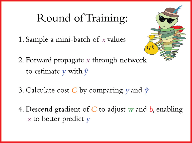
Figure 8.5 An individual round of training with stochastic gradient descent. Although mini-batch size is a hyperparameter that can vary, in this particular case, the mini-batch consists of 128 MNIST digits, as exemplified by our hike-loving trilobite carrying a small bag of data.
Figure 8.6 captures how rounds of training are repeated until we run out of training images to sample. The sampling in step 1 is done without replacement, meaning that at the end of an epoch each image has been seen by the algorithm only once, and yet between different epochs the mini-batches are sampled randomly. After a total of 468 rounds, the final batch contains only 96 samples.
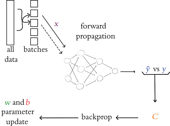
Figure 8.6 An outline of the overall process for training a neural network with stochastic gradient descent. The entire dataset is shuffled and split into batches. Each batch is forward propagated through the network; the output ŷ is compared to the ground truth y and the cost C is calculated; backpropagation calculates the gradients; and the model parameters w and b are updated. The next batch (indicated by a dashed line) is forward propagated, and so on until all of the batches have moved through the network. Once all the batches have been used, a single epoch is complete and the process starts again with a reshuffling of the full training dataset.
This marks the end of the first epoch of training. Assuming we’ve set our model up to train for further epochs, we begin the next epoch by replenishing our pool with all 60,000 training images. As we did through the previous epoch, we then proceed through a further 469 rounds of stochastic gradient descent.11 Training continues in this way until the total desired number of epochs is reached.
11. Because we’re sampling randomly, the order in which we select training images for our 469 mini-batches is completely different for every epoch.
The total number of epochs that we set our network to train for is yet another hyperparameter, by the way. This hyperparameter, though, is one of the easiest to get right:
If the cost on your validation data is going down epoch over epoch, and if your final epoch attained the lowest cost yet, then you can try training for additional epochs.
Once the cost on your validation data begins to creep upward, that’s an indicator that your model has begun to overfit to your training data because you’ve trained for too many epochs. (We elaborate much more on overfitting in Chapter 9.)
There are methods12 you can use to automatically monitor training and validation cost and stop training early if things start to go awry. In this way, you could set the number of epochs to be arbitrarily large and know that training will continue until the validation cost stops improving—and certainly before the model begins overfitting!
12. See keras.io/callbacks/#earlystopping.
Escaping the Local Minimum
In all of the examples of gradient descent thus far in the chapter, our hiking trilobite has encountered no hurdles on its journey toward minimum cost. There are no guarantees that this would be the case, however. Indeed, such smooth sailing is unusual.
Figure 8.7 shows the mountaineering trilobite exploring the cost of some new model that is being used to solve some new problem. With this new problem, the relationship between the parameter p and cost C is more complex. To have our neural network estimate y as accurately as possible, gradient descent needs to identify the parameter values associated with the lowest-attainable cost. However, as our trilobite makes its way from its random starting point in the top panel, gradient descent leads it to getting trapped in a local minimum. As shown in the middle panel, while our intrepid explorer is in the local minimum, a step to the left or a step to the right both lead to an increase in cost, and so the blind trilobite stays put, completely oblivious of the existence of a deeper valley—the global minimum—lying yonder.
All is not lost, friends, for stochastic gradient descent comes to the rescue here again. The sampling of mini-batches can have the effect of smoothing out the cost curve, as exemplified by the dashed curve shown in the bottom panel of Figure 8.7. This smoothing happens because the estimate is noisier when estimating the gradient from a smaller mini-batch (versus from the entire dataset). Although the actual gradient in the local minimum truly is zero, estimates of the gradient from small subsets of the data don’t provide the complete picture and might give an inaccurate reading, causing our trilobite to take a step left thinking there is a gradient when there really isn’t one. This noisiness and inaccuracy is paradoxically a good thing! The incorrect gradient may result in a step that is large enough for the trilobite to escape the local valley and continue making its way down the mountain. Thus, by estimating the gradient many times on these mini-batches, the noise is smoothed out and we are able to avoid local minima. In summary, although each mini-batch on its own lacks complete information about the cost curve, in the long run—over a large number of mini-batches—this tends to work to our advantage.
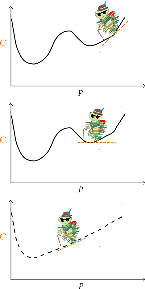
Figure 8.7 A trilobite applying vanilla gradient descent from a random starting point (top panel) is ensnared by a local minimum of cost (middle panel). By turning to stochastic gradient descent in the bottom panel, the daring trilobite is able to bypass the local minimum and make its way toward the global minimum.
Like the learning rate hyperparameter η, there is also a Goldilocks-style sweet spot for batch size. If the batch size is too large, the estimate of the gradient of the cost function is far more accurate. In this way, the trilobite has a more exacting impression of the gradient in its immediate vicinity and is able to take a step (proportional to η) in the direction of the steepest possible descent. However, the model is at risk of becoming trapped in local minima as described in the preceding paragraph.13 Besides that, the model might not fit in memory on your machine, and the compute time per iteration of gradient descent could be very long.
13. It’s worth noting that the learning rate η plays a role here. If the size of the local minimum was smaller than the step size, the trilobite would likely breeze right past the local minimum, akin to how we step over cracks in the sidewalk.
On the other hand, if the batch size is too small, each gradient estimate may be excessively noisy (because a very small subset of the data is being used to estimate the gradient of the entire dataset) and the corresponding path down the mountain will be unnecessarily circuitous; training will take longer because of these erratic gradient descent steps. Furthermore, you’re not taking advantage of the memory and compute resources on your machine.14 With that in mind, here are our rules of thumb for finding the batch-size sweet spot:
Start with a batch size of 32.
If the mini-batch is too large to fit into memory on your machine, try decreasing your batch size by powers of 2 (e.g., from 32 to 16).
If your model trains well (i.e., cost is going down consistently) but each epoch is taking very long and you are aware that you have RAM to spare,15 you could experiment with increasing your batch size. To avoid getting trapped in local minima, we don’t recommend going beyond 128.
14. Stochastic gradient descent with a batch size of 1 is known as online learning. It’s worth noting that this is not the fastest method in terms of compute. The matrix multiplication associated with each round of mini-batch training is highly optimized, and so training can be several orders of magnitude quicker when using moderately sized mini-batches relative to online learning.
15. On a Unix-based operating system, including macOS, RAM usage may be assessed by running the top or htop command within a Terminal window.
Backpropagation
Although stochastic gradient descent operates well on its own to adjust parameters and minimize cost in many types of machine learning models, for deep learning models in particular there is an extra hurdle: We need to be able to efficiently adjust parameters through multiple layers of artificial neurons. To do this, stochastic gradient descent is partnered up with a technique called backpropagation.
Backpropagation—or backprop for short—is an elegant application of the “chain rule” from calculus.16 As shown along the bottom of Figure 8.6 and as suggested by its very name, backpropagation courses through a neural network in the opposite direction of forward propagation. Whereas forward propagation carries information about the input x through successive layers of neurons to approximate y with ŷ, backpropagation carries information about the cost C backwards through the layers in reverse order and, with the overarching aim of reducing cost, adjusts neuron parameters throughout the network.
16. To elucidate the mathematics underlying backpropagation, a fair bit of partial-derivative calculus is necessary. While we encourage the development of an in-depth understanding of the beauty of backprop, we also appreciate that calculus might not be the most appetizing topic for everyone. Thus, we’ve placed our content on backprop mathematics in Appendix B.
Although the nitty-gritty of backpropagation has been relegated to Appendix B, it’s worth understanding (in broad strokes) what the backpropagation algorithm does: Any given neural network model is randomly initialized with parameter (w and b) values (such initialization is detailed in Chapter 9). Thus, prior to any training, when the first x value is fed in, the network outputs a random guess at ŷ. This is unlikely to be a good guess, and the cost associated with this random guess will probably be high. At this point, we need to update the weights in order to minimize the cost—the very essence of machine learning. To do this within a neural network, we use backpropagation to calculate the gradient of the cost function with respect to each weight in the network.
Recall from our mountaineering analogies earlier that the cost function represents a hiking trail, and our trilobite is trying to reach basecamp. At each step along the way, the trilobite finds the gradient (or the slope) of the cost function and moves down that gradient. That movement corresponds to a weight update: By adjusting the weight in proportion to the cost function’s gradient with respect to that weight, backprop adjusts that weight in a direction that reduces the cost.
Reflecting back on the “most important equation” from Figure 6.7 (w · x + b), and remembering that neural networks are stacked with information forward propagating through their layers, we can grasp that any given weight in the network contributes to the final ŷ output, and thus the cost C. Using backpropagation, we move layer-by-layer backwards through the network, starting at the cost in the output layer, and we find the gradients of every single parameter. A given parameter’s gradient can then be used to adjust the parameter up or down (by an increment corresponding to the learning rate η)—whichever of the two directions is associated with a reduction in cost.
We appreciate that this is not the lightest section of this book. If there’s only one thing you take away, let it be this: Backpropagation uses cost to calculate the relative contribution by every single parameter to the total cost, and then it updates each parameter accordingly. In this way, the network iteratively reduces cost and, well . . . learns!
Tuning Hidden-Layer Count and Neuron Count
As with learning rate and batch size, the number of hidden layers you add to your neural network is also a hyperparameter. And as with the previous two hyperparameters, there is yet again a Goldilocks sweet spot for your network’s count of layers. Throughout this book, we’ve reiterated that with each additional hidden layer within a deep learning network, the more abstract the representations that the network can represent. That is the primary advantage of adding layers.
The disadvantage of adding layers is that backpropagation becomes less effective: As demonstrated by the plot of learning speed across the layers of a five-hidden-layer network in Figure 8.8, backprop is able to have its greatest impact on the parameters of the hidden layer of neurons closest to the output ŷ.17 The farther a layer is from ŷ, the more diluted the effect of that layer’s parameters on the overall cost. Thus, the fifth layer, which is closest to the output ŷ, learns most rapidly because those weights are associated with larger gradients. In contrast, the third hidden layer, which is several layers away from the output layer’s cost calculation, learns about an order of magnitude more slowly than the fifth hidden layer.
17. If you’re curious as to how we made Figure 8.8, check out our Measuring Speed of Learning Jupyter notebook.
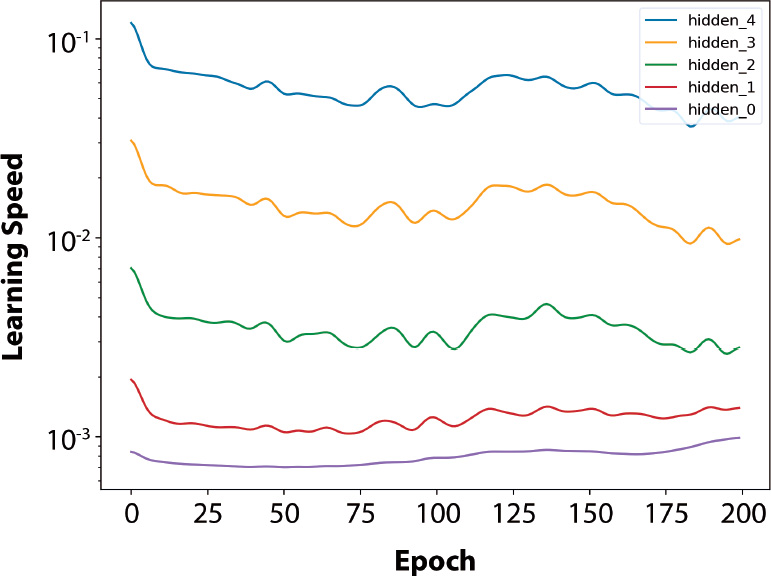
Figure 8.8 The speed of learning over epochs of training for a deep learning network with five hidden layers. The fifth hidden layer, which is closest to the output ŷ, learns about an order of magnitude more quickly than the third hidden layer.
Given the above, our rules of thumb for selecting the number of hidden layers in a network are:
The more abstract the ground-truth value y you’d like to estimate with your network, the more helpful additional hidden layers may be. With that in mind, we recommend starting off with about two to four hidden layers.
If reducing the number of layers does not increase the cost you can achieve on your validation dataset, then do it. Following the problem-solving principle called Occam’s razor, the simplest network architecture that can provide the desired result is the best; it will train more quickly and require fewer compute resources.
On the other hand, if increasing the number of layers decreases the validation cost, then you should pile up those layers!
Not only is network depth a model hyperparameter, but the number of neurons in a given layer is, too. If you have many layers in your network, then there are many layers you could be fine-tuning your neuron count in. This may seem intimidating at first, but it’s nothing to be too concerned about: A few too many neurons, and your network will have a touch more computational complexity than is necessary; a touch too few neurons, and your network’s accuracy may be held back imperceptibly.
As you build and train more and more deep learning models for more and more problems, you’ll begin to develop a sense for how many neurons might be appropriate in a given layer. Depending on the particular data you’re modeling, there may be lots of low-level features to represent, in which case you might want to have more neurons in the network’s early layers. If there are lots of higher-level features to represent, then you may benefit from having additional neurons in its later layers. To determine this empirically, we generally experiment with the neuron count in a given layer by varying it by powers of 2. If doubling the number of neurons from 64 to 128 provides an appreciable improvement in model accuracy, then go for it. Rehashing Occam’s razor, however, consider this: If halving the number of neurons from 64 to 32 doesn’t detract from model accuracy, then that’s probably the way to go because you’re reducing your model’s computational complexity with no apparent negative effects.
An Intermediate Net in Keras
To wrap up this chapter, let’s incorporate the new theory we’ve covered into a neural network to see if we can outperform our previous Shallow Net in Keras model at classifying handwritten digits.
The first few stages of our Intermediate Net in Keras Jupyter notebook are identical to those of its Shallow Net predecessor. We load the same Keras dependencies, load the MNIST dataset in the same way, and preprocess the data in the same way. As shown in Example 8.1, the situation begins to get interesting when we design our neural network architecture.
Example 8.1 Keras code to architect an intermediate-depth neural network
model = Sequential()
model.add(Dense(64, activation='relu', input_shape=(784,)))
model.add(Dense(64, activation='relu'))
model.add(Dense(10, activation='softmax'))
The first line of this code chunk, model = Sequential(), is the same as before (refer to Example 5.6); this is our instantiation of a neural network model object. It’s in the second line that we begin to diverge. In it, we specify that we’ll substitute the sigmoid activation function in the first hidden layer with our most-highly-recommended neuron from Chapter 6, the relu. Other than this activation function swap, the first hidden layer remains the same: It still consists of 64 neurons, and the dimensionality of the 784-neuron input layer is unchanged.
The other significant change in Example 8.1 relative to the shallow architecture of Example 5.6 is that we specify a second hidden layer of artificial neurons. By calling the model.add() method, we nearly effortlessly add a second Dense layer of 64 relu neurons, providing us with the notebook’s namesake: an intermediate-depth neural network. With a call to model.summary(), you can see from Figure 8.9 that this additional layer corresponds to an additional 4,160 trainable parameters relative to our shallow architecture (refer to Figure 7.5). We can break these parameters down into:
4,096 weights, corresponding to each of the 64 neurons in the second hidden layer densely receiving input from each of the 64 neurons in the first hidden layer (64 × 64 = 4,096)
Plus 64 biases, one for each of the neurons in the second hidden layer
Giving us a total of 4,160 parameters: nparameters = nw + nb = 4,096 + 64 = 4,160
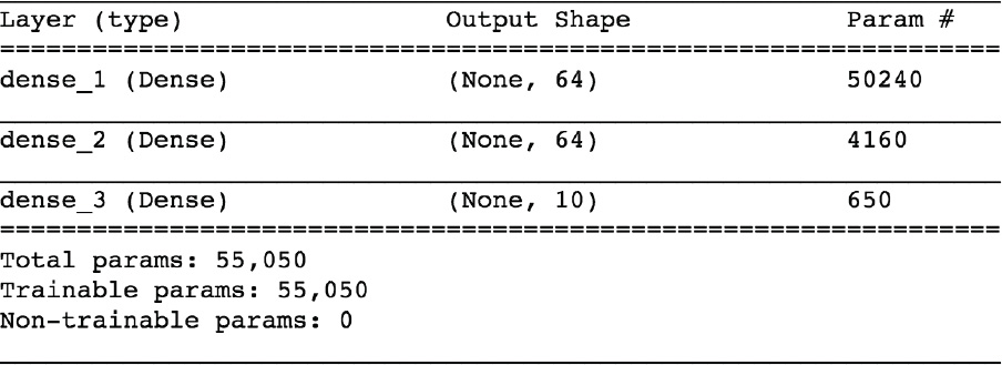
Figure 8.9 A summary of the model object from our Intermediate Net in Keras Jupyter notebook
In addition to changes to the model architecture, we’ve also made changes to the parameters we specify when compiling our model, as shown in Example 8.2.
Example 8.2 Keras code to compile our intermediate-depth neural network
model.compile(loss='categorical_crossentropy',
              optimizer=SGD(lr=0.1),
              metrics=['accuracy'])
With these lines from Example 8.2, we:
Set our loss function to cross-entropy cost by using
loss='categorical_crossentropy'(in Shallow Net in Keras, we used quadratic cost by usingloss='mean_squared_error')Set our cost-minimizing method to stochastic gradient descent by using
optimizer=SGDSpecify our SGD learning rate hyperparameter η by setting
lr=0.118Indicate that, in addition to the Keras default of providing feedback on
loss, by settingmetrics=['accuracy'], we’d also like to receive feedback on model accuracy19
18. On your own time, you can play around with increasing this learning rate by several orders of magnitude as well as decreasing it by several orders of magnitude, and observing how it impacts training.
![]()
19. Although loss provides the most important metric for tracking a model’s performance epoch over epoch, its particular values are specific to the characteristics of a given model and are not generally interpretable or comparable between models. Because of this, other than knowing that we would like our loss to be as close to zero as possible, it can be an esoteric exercise to interpret how close to zero loss should be for any particular model. Accuracy, on the other hand, is highly interpretable and highly generalizable: We know exactly what it means (e.g., “The shallow neural network correctly classified 86 percent of the handwritten digits in the validation dataset”), and we can compare this classification accuracy to any other model (“The accuracy of 86 percent is worse than the accuracy of our deep neural network”).
Finally, we train our intermediate net by running the code in Example 8.3.
Example 8.3 Keras code to train our intermediate-depth neural network
model.fit(X_train, y_train,
          batch_size=128, epochs=20,
          verbose=1,
          validation_data=(X_valid, y_valid))
Relative to the way we trained our shallow net (see Example 5.7), the only change we’ve made is reducing our epochs hyperparameter from 200 down by an order of magnitude to 20. As you’ll see, our much-more-efficient intermediate architecture required far fewer epochs to train.
Figure 8.10 provides the results of the first three epochs of training the network. Recalling that our shallow architecture plateaued as it approached 86 percent accuracy on the validation dataset after 200 epochs, our intermediate-depth network is clearly superior: The val_acc field shows that we attained 92.34 percent accuracy after a single epoch of training. This accuracy climbs to more than 95 percent by the third epoch and appears to plateau around 97.6 percent by the twentieth. My, how far we’ve come already!
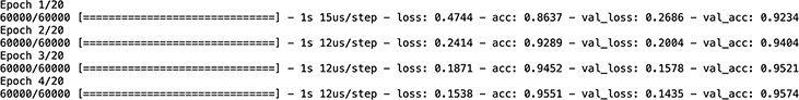
Figure 8.10 The performance of our intermediate-depth neural network over its first four epochs of training
Let’s break down the verbose model.fit() output shown in Figure 8.10 in further detail:
The progress bar shown next fills in over the course of the 469 “rounds of training” (Figure 8.5):
60000/60000 [==============================]
1s 15us/stepindicates that all 469 rounds in the first epoch required 1 second to train, at an average rate of 15 microseconds per round.lossshows the average cost on our training data for the epoch. For the first epoch this is0.4744, and, epoch over epoch, this cost is reliably minimized via stochastic gradient descent (SGD) and backpropagation, eventually diminishing to0.0332by the twentieth epoch.accis the classification accuracy on training data for the epoch. The model correctly classified 86.37 percent for the first epoch, increasing to more than 99 percent by the twentieth. Because a model can overfit to the training data, one shouldn’t be overly impressed by high accuracy on the training data.Thankfully, our cost on the validation dataset (
val_loss) does generally decrease as well, eventually plateauing as it approaches 0.08 over the final five epochs of training.Corresponding to the decreasing cost of the validation data is an increase in accuracy (
val_acc). As mentioned, validation accuracy plateaued at about 97.6 percent, which is a vast improvement over the 86 percent of our shallow net.
Summary
We covered a lot of ground in this chapter. Starting from an appreciation of how a neural network with fixed parameters processes information, we developed an understanding of the cooperating methods—cost functions, stochastic gradient descent, and backpropagation—that enable network parameters to be learned so that we can approximate any y that has a continuous relationship to some input x. Along the way, we introduced several network hyperparameters, including learning rate, mini-batch size, and number of epochs of training—as well as our rules of thumb for configuring each of these. The chapter concluded by applying your newfound knowledge to develop an intermediate-depth neural network that greatly outperformed our previous, shallow network on the same handwritten-digit-classification task. Up next, we have techniques for improving the stability of artificial neural networks as they deepen, enabling you to architect and train a bona fide deep learning model for the first time.
Key Concepts
Here are the essential foundational concepts thus far. New terms from the current chapter are highlighted in purple.
parameters:
weight w
bias b
activation a
artificial neurons:
sigmoid
tanh
ReLU
input layer
hidden layer
output layer
layer types:
dense (fully connected)
softmax
cost (loss) functions:
quadratic (mean squared error)
cross-entropy
forward propagation
backpropagation
optimizers:
stochastic gradient descent
optimizer hyperparameters:
learning rate η
batch size