
10. Machine Vision
Welcome to Part III, dear reader. Previously, we provided a high-level overview of particular applications of deep learning (Part I). With the foundational, low-level theory we’ve covered since (in Part II), you’re now well positioned to work through specialized content across a range of application areas, primarily via hands-on example code. In this chapter, for example, you’ll discover convolutional neural networks and apply them to machine vision tasks. In the remainder of Part III, we cover practical examples of:
Recurrent neural networks for natural language processing in Chapter 11
Generative adversarial networks for visual creativity in Chapter 12
Deep reinforcement learning for sequential decision making within complex, changing environments in Chapter 13
Convolutional Neural Networks
A convolutional neural network—also known as a ConvNet or a CNN—is an artificial neural network that features one or more convolutional layers (also called conv layers). This layer type enables a deep learning model to efficiently process spatial patterns. As you’ll see firsthand in this chapter, this property makes convolutional layers especially effective in computer vision applications.
The Two-Dimensional Structure of Visual Imagery
In our previous code examples involving handwritten MNIST digits, we converted the image data into one-dimensional arrays of numbers so that we could feed them into a dense hidden layer. More specifically, we began with 28×28-pixel grayscale images and converted them into 784-element one-dimensional arrays.1 Although this step was necessary in the context of a dense, fully connected network—we needed to flatten the 784 pixel values so that each one could be fed into a neuron of the first hidden layer—the collapse of a two-dimensional image into one dimension corresponds to a substantial loss of meaningful visual image structure. When you draw a digit with a pen on paper, you don’t conceptualize it as a continuous linear sequence of pixels running from top-left to bottom-right. If, for example, we printed an MNIST digit for you here as a 784-pixel long stream in shades of gray, we’d be willing to wager that you couldn’t identify the digit. Instead, humans perceive visual information in a two-dimensional form,2 and our ability to recognize what we’re looking at is inherently tied to the spatial relationships between the shapes and colors we perceive.
1. Recall that the pixel values were divided by 255 in order to scale everything to [0 : 1].
2. Well . . . three-dimensional, but let’s ignore depth for the purposes of this discussion.
Computational Complexity
In addition to the loss of two-dimensional structure when we collapse an image, a second consideration when piping images into a dense network is computational complexity. The MNIST images are very small—28×28 pixels with only one channel (there is only one color “channel” because MNIST digits are monochromatic; to render images in full color, in contrast, at least three channels—usually red, green, and blue—are required). Passing MNIST image information into a dense layer, that corresponds to 785 parameters per neuron: 784 weights for each of the pixels, plus the neuron’s bias. If we were handling a moderately sized image, however—say, a 200×200-pixel, full-color RGB3 image—then the number of parameters increases dramatically. In that case, we’d have three color channels, each with 40,000 pixels, corresponding to a total of 120,001 parameters per neuron in a dense layer.4 With a modest number of neurons in the dense layer—let’s say 64—that corresponds to nearly 8 million parameters associated with the first hidden layer of our network alone.5 Furthermore, the image is only 200×200 pixels—that’s barely 0.4MP,6 whereas most modern smartphones have 12MP or greater camera sensors. Generally, machine vision tasks don’t need to run on high-resolution images in order to be successful, but the point should be clear: Images can contain a very large number of data points, and using these in a naïve, fully connected manner will explode the neural network’s compute power requirements.
3. The red, green, and blue channels required for a full-color image.
4. 200 pixels × 200 pixels × 3 color channels + 1 bias = 120,001 parameters.
5. 64 neurons × 120,001 parameters per neuron = 7,680,064 parameters.
6. Megapixels.
Convolutional Layers
Convolutional layers consist of sets of kernels, which are also known as filters. Each of these kernels is a small window (called a patch) that scans across the image (in more technical terms, the filter convolves), from top left to bottom right (see Figure 10.1 for an illustration of this convolutional operation).
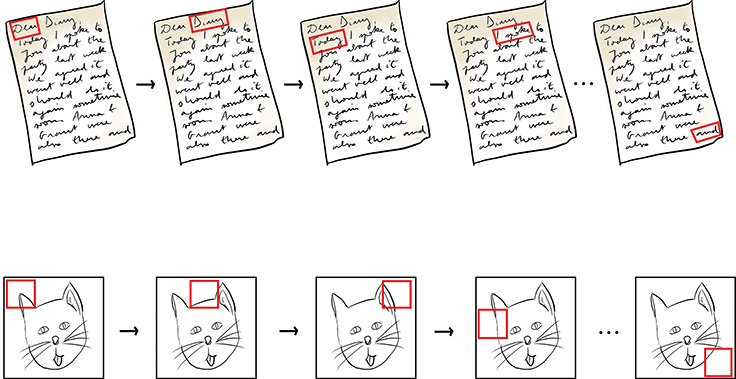
Figure 10.1 When reading a page of a book written in English, we begin in the top-left corner and read to the right. Every time we reach the end of a row of text, we progress to the next row. In this way, we eventually reach the bottom-right corner, thereby reading all of the words on the page. Analogously, the kernel in a convolutional layer begins on a small window of pixels in the top-left corner of a given image. From the top row downward, the kernel scans from left to right, until it eventually reaches the bottom-right corner, thereby scanning all of the pixels in the image.
Kernels are made up of weights, which—as in dense layers—are learned through back-propagation. Kernels can range in size, but a typical size is 3×3, and we use that in the examples in this chapter.7 For the monochromatic MNIST digits, this 3×3-pixel window would consist of 3 × 3 × 1 weights—nine weights, for a total of 10 parameters (like an artificial neuron in a dense layer, every convolutional filter has a bias term b). For comparison, if we happened to be working with full-color RGB images, then a kernel covering the same number of pixels would have three times as many weights—3 × 3 × 3 of them, for a total of 27 weights and 28 parameters.
7. Another typical size is 5×5, with kernels larger than that used infrequently.
As depicted in Figure 10.1, the kernel occupies discrete positions across an image as it convolves. Sticking with the 3×3 kernel size for this explanation, during forward propagation a multidimensional variation of the “most important equation in this book”—w · x + b (introduced in Figure 6.7)—is calculated at each position that the kernel occupies as it convolves over the image. Referring to the 3×3 window of pixels and the 3×3 kernel in Figure 10.2 as inputs x and weights w, respectively, we can demonstrate the calculation of the weighted sum w · x in which products are calculated elementwise based on the alignment of vertical and horizontal locations. It’s helpful to imagine the kernel superimposed over the pixel values. The math is presented here:
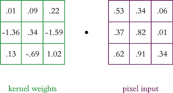
Figure 10.2 A 3×3 kernel and a 3×3-pixel window
Next, using Equation 7.1, we add some bias term b (say, –0.19) to arrive at z:
With z, we can at last calculate an activation value a by passing z through the activation function of our choice, say the tanh function or the ReLU function.
Note that the fundamental operation hasn’t changed relative to the artificial neuron mathematics of Chapters 6 and 7. Convolutional kernels have weights, inputs, and a bias; a weighted sum of these is produced using our most important equation; and the resulting z is passed through some nonlinear function to produce an activation. What has changed is that there isn’t a weight for every input, but rather a discrete kernel with 3×3 weights. These weights do not change as the kernel convolves; instead they’re shared across all of the inputs. In this way, a convolutional layer can have orders of magnitude fewer weights than a fully connected layer. Another important point is that, like the inputs, the outputs from this kernel (all of the activations) are also arranged in a two-dimensional array. We’ll delve more into this in a moment, but first . . .
Multiple Filters
Typically, we have multiple filters in a given convolutional layer. Each filter enables the network to learn a representation of the data at a given layer in a unique way. For example, analogous to Hubel and Wiesel’s simple cells in the biological visual system (Figure 1.5), if the first hidden layer in our network is a convolutional layer, it might contain a kernel that responds optimally to vertical lines. Thus, whenever it convolves (slides over) a vertical line in an input image, it produces a large activation (a) value. Additional kernels in this layer can learn to represent other simple spatial features such as horizontal lines and color transitions (for examples, see the bottom-left panel of Figure 1.17). This is how these kernels came to be known as filters; they scan over the image and filter out the location of specific features, producing high activations when they come across the pattern, shape, and/or color they are specially tuned to detect. One could say that they function as highlighters, producing a two-dimensional array of activations that indicate where that filter’s particular feature exists in the original image. For this reason, the output from a kernel is referred to as an activation map.
Analogous to the hierarchical representations of the biological visual system (Figure 1.6), subsequent convolutional layers receive these activation maps as their inputs. As the network gets deeper, the filters in the layers react to increasingly complex combinations of these simple features, learning to represent increasingly abstract spatial patterns and eventually building a hierarchy from simple lines and colors up to complex textures and shapes (see the panels along the bottom of Figure 1.17). In this way, later layers within the network have the capacity to recognize whole objects or even, say, to distinguish an image of a Great Dane from that of a Yorkshire Terrier.
The number of filters in the layer, like the number of neurons in a dense layer, is a hyperparameter that we configure ourselves. As with the other hyperparameters covered already in this book, there is a Goldilocks sweet spot for filter number. Here are our rules of thumb for homing in on it for your particular problem:
Having a larger number of kernels facilitates the identification of more-complex features, so consider the complexity of the data and the problem you’re solving. Of course, more kernels comes with the cost of computation efficiency.
If a network has multiple convolutional layers, the optimal number of kernels for a given layer could vary quite a bit from layer to layer. Keep in mind that early layers identify simple features, whereas later layers identify complex recombinations of these simple features, so let this guide where you stack your network. As we’ll see when we get into coded examples of CNNs later in this chapter, a common approach for machine vision is to have many more kernels in later convolutional layers relative to early convolutional layers.
As always, strive to minimize computational complexity: Consider using the smallest number of kernels that facilitates a low cost on your validation data. If doubling the number of kernels (say, from 32 to 64 to 128) in a given layer significantly decreases your model’s validation cost, then consider using the higher value. If halving the number of kernels (say, from 32 to 16 to 8) in a given layer doesn’t increase your model’s validation cost, then consider using the smaller value.
A Convolutional Example
Convolutional layers are a nontrivial departure from the simpler fully connected layers of Part II, so, to help you make sense of the way the pixel values and weights combine to produce feature maps, across Figures 10.3 through 10.5 we’ve created a detailed contrived example with accompanying math. To begin, imagine we’re convolving over a single RGB image that’s 3×3 pixels in size. In Python, those data are stored in a [3,3,3] array as shown at the top of Figure 10.3.8
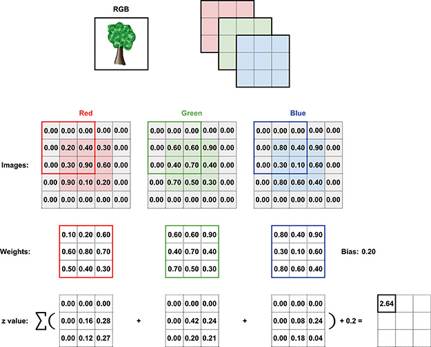
Figure 10.3 This schematic diagram demonstrates how the activation values in a feature map are calculated in a convolutional layer.
8. We admit that the RGB example of the tree has far more than nine pixels, but we struggled to identify a compelling color image that was 3×3.
Shown in the middle of the figure are the 3×3 arrays for each of the three channels: red, green, and blue. Note that the image has been padded with zeros on all four sides. We’ll discuss more about padding shortly, but for now all you need to know is this: Padding is used to ensure that the resulting feature map has the same dimensions as the input data. Below the arrays of pixel values you’ll find the weight matrices for each of the channels. We chose a kernel size of 3×3, and given that there are three channels in the input image the weights matrix will be an array with dimensions [3,3,3], shown here individually. The bias term is 0.2. The current position of the filter is indicated by an overlay on each array of pixel values, and the z value (determined by calculating the weighted sum from Equation 10.1 across all three color channels, and then adding the bias as in Equation 10.2) is given at the bottom right of the figure. Finally, all of these z values are summed to create the first entry in the feature map at the bottom right.
Proceeding to Figure 10.4, the image arrays are now shown with the filter in its next position, one pixel to the right. Exactly as in Figure 10.3, the z value is calculated following Equations 10.1 and 10.2. This z-value can then fill the second position in the activation map, as shown again at the bottom right of the figure.
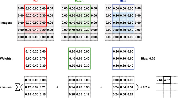
Figure 10.4 A continuation of the convolutional example from Figure 10.3, now showing the activation for the next filter position
This process is repeated for every possible filter position, and the z-value that was calculated for each of these nine positions is shown in the bottom-right corner of Figure 10.5. To convert this 3×3 map of z-values into a corresponding 3×3 activation map, we pass each z-value through an activation function, such as the ReLU function. Because a single convolutional layer nearly always has multiple filters, each producing its own two-dimensional activation map, activation maps have an additional depth dimension, analogous to the depth provided by the three the channels of an RGB image. Each of these kernel “channels” in the activation map represents a feature that that particular kernel specializes in recognizing, such as an edge (a straight line) at a particular orientation.9 Figure 10.6 shows how the calculation of activation values a from the input image build up a three-dimensional activation map. The convolutional layer that produced the activation map shown in Figure 10.6 has 16 kernels, thus resulting in an activation map with a depth of 16 “channels” (we’ll call these slices going forward).

Figure 10.5 Finally, the activation for the last filter position has been calculated, and the activation map is complete.
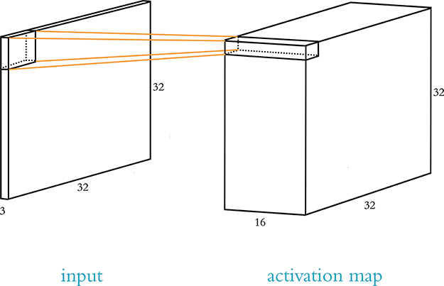
Figure 10.6 A graphical representation of the input array (left; represented here is a three-channel RGB image of size 32×32 with the kernel patch currently focused on the first—i.e., top-left—position) and the activation map (right). There are 16 kernels, resulting in an activation map with a depth of 16. Each position a given kernel occupies as it convolves over the input image corresponds to one a value in the resulting activation map.
9. Figure 1.17 shows real-world examples of the features individual kernels become specialized to detect across a range of convolutional-layer depths. In the first convolutional layer, for example, the majority of the kernels have a speciality in detecting an edge at a particular orientation.
In Figure 10.6, the kernel filter is positioned over the top-left corner of the input image. This corresponds to 16 activation values in the top-left corner of the activation map: one activation a for each of the 16 kernels. By convolving over all of the pixel windows in the input image from left to right and from top to bottom, all of the values in the activation map are filled in.10 If the first of the 16 filters is tuned to respond optimally to vertical lines, then the first slice of the activation map will highlight all the physical regions of the input image that contain vertical lines. If the second filter is tuned to respond optimally to horizontal lines, then the second slice of the activation map will highlight regions of the image that contain horizontal lines. In this way, all 16 filters in the activation map can together represent the spatial location of 16 different spatial features.11
![]()
10. Note that regardless of whether an input image is monochromatic (with only one color channel) or full-color (with three), there is only one activation map output for each convolutional kernel. If there is one color channel, we calculate the weighted sum of inputs for that single channel as in Equation 10.1. If there are three color channels, we calculate the total weighted sum of inputs across all three channels as in Figures 10.3, 10.4, and 10.5. Either way (after adding the kernel’s bias and passing the resulting z-value through an activation function), we produce only one activation value for each position that each kernel convolves over.
11. If you are interested in an interactive demonstration of convolutional-filter calculations, we highly recommend one created by Andrej Karpathy (see Figure 14.6 for a portrait). It’s available at bit.ly/CNNdemo under the Convolution Demo heading.
![]()
12. Yosinski, J., et al. (2015). Understanding neural networks through deep visualization. Proceedings of the International Conference on Machine Learning.
Now that we’ve described the general principles underscoring convolutional layers in deep learning, it’s a good time to review the basic features:
They allow deep learning models to learn to recognize features in a position invariant manner; a single kernel can identify its cognate feature anywhere in the input data.
They remain faithful to the two-dimensional structure of images, allowing features to be identified within their spacial context.
They significantly reduce the number of parameters required for modeling image data, yielding higher computational efficiency.
Ultimately, they perform machine vision tasks (e.g., image classification) more accurately.
Convolutional Filter Hyperparameters
In contrast with dense layers, convolutional layers are inherently not fully connected. That is, there isn’t a weight mapping every single pixel to every single neuron in the first hidden layer. Instead, there are a handful of hyperparameters that dictate the number of weights and biases associated with a given convolutional layer. These include:
Kernel size
Stride length
Padding
Kernel Size
In all of the examples covered so far in this chapter, the kernel size (also known as filter size or receptive field13) has been 3 pixels wide and 3 pixels tall. This is a common size that is found to be effective across a broad range of machine vision applications in contemporary ConvNet architectures. A kernel size of 5×5 pixels is also popular, and 7×7 is about as expansive as they ever get. If the kernel is too large with respect to the image, there would be too many competing features in the receptive field and it would be challenging for the convolutional layer to learn effectively, but if the receptive field is too small (e.g., 2×2) it wouldn’t be able to tune to any structures, and that isn’t helpful either.
13. The term receptive field is borrowed directly from the study of biological visual systems like the eye.
Stride Length
Stride refers to the size of the step that the kernel takes as it moves over the image. Across our convolutional-layer example (Figures 10.3 to 10.5) we use a stride length of 1 pixel, which is a frequently used option. Another common choice is a 2-pixel stride and, less often, a stride of 3. Anything much larger is likely to be suboptimal, because the kernel might skip regions of the image that are of value to the model. On the other hand, increasing the stride will yield an increase in speed because there are fewer calculations that need to be carried out. As ever in deep learning, it’s about finding a balance—that Goldilocks sweet spot—between these effects. We recommend a stride of 1 or 2, while avoiding anything larger than 3.
Padding
Next is padding, which plays handily with stride to keep the calculations of a convolutional layer in order. Let’s suppose you had a 28×28 MNIST digit and a 5×5 kernel. With a stride of 1, there are 24×24 “positions” for the kernel to move through before it bumps up against the edges of the image, so the activation map output by the layer is slightly smaller than the input. If you’d like to produce an activation map that is the exact same size as the input image, you can simply pad the image with zeros around the edges (Figures 10.3, 10.4, and 10.5 contain an example of a zero-padded image). In the case of the 28×28 image and the 5×5 kernel, padding with two zeros on each edge will produce a 28×28 activation map. This can be calculated with the following equation:
Where:
D is the size of the image (either width or height, depending on whether you’re calculating the width or height of the activation map).
F is the size of the filter.
P is the amount of padding.
S is the stride length.
Thus, with our padding of 2, we can calculate that the output volume is 28 × 28:
Given the interconnected nature of kernel size, stride, and padding, one has to make sure these hyperparameters align when designing CNN architectures. That is, the hyper-parameters must combine to produce a valid activation map size—specifically, an integer value. Take, for example, a kernel size of 5 × 5 with a stride of 2 and no padding. Using Equation 10.3, this would result in a 12.5×12.5 activation map:
There is no such thing as a partial activation value, so a convolutional layer with these dimensions would simply not be computable.
Pooling Layers
Convolutional layers frequently work in tandem with another layer type that is a staple in machine vision neural networks: pooling layers. This layer type serves to reduce the overall count of parameters in a network as well as to reduce complexity, thereby speeding up computation and helping to avoid overfitting.
As discussed in the preceding section, a convolutional layer can have any number of kernels. Each of these kernels produces an activation map (whose dimensions are defined by Equation 10.3), such that the output from a convolutional layer is a three-dimensional array of activation maps, with the depth dimension of the output corresponding to the number of filters in that convolutional layer. The pooling layer reduces these activation maps spatially, while leaving the depth of the activation maps intact.
Like convolutional layers, any given pooling layer has a filter size and a stride length. Also like a convolutional layer, the pooling layer slides over its input. At each position it occupies, the pooling layer applies a data-reducing operation. Pooling layers most often use the max operation, and these are termed max-pooling layers: They retain the largest value (the maximum activation) within the receptive field while discarding the other values (see Figure 10.7).14 Typically, a pooling layer has a filter size of 2 × 2 and a stride length of 2.15 In this case, at each position the pooling layer evaluates four activations, retaining only the maximum value, and thereby downsampling the activations by a factor of 4. Because this pooling operation happens independently for each depth slice in the three-dimensional array, a 28 × 28 activation map with a depth of 16 slices would be reduced to a 14 × 14 activation map but it would retain its full complement of 16 slices.
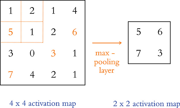
Figure 10.7 An example of a max-pooling layer being passed a 4×4 activation map. Like a convolutional layer, the pooling layer slides from left to right and from top to bottom over the matrix of values input into it. With a 2×2-sized filter, the layer retains only the largest of four input values (e.g., the orange “5” in the 2×2 hatch-marked top-left corner). With a 2×2 stride, the resulting output from this max-pooling layer has one-quarter of the volume of its input: a 2×2 activation map.
14. Other pooling variants (e.g., average pooling, L2-norm pooling) exist but are much less common relative to max-pooling, which typically suits machine vision applications sufficiently accurately while requiring minimal computational resources (it is, for example, more computationally expensive to calculate an average than a maximum).
15. Max-pooling with a filter size of 2 × 2 with a stride of 2 is our default recommendation. Both, however, are hyperparameters that you can experiment with, if desired.
![]()
LeNet-5 in Keras
All the way back at Figure 1.11, as we introduced the hierarchical nature of deep learning, we discussed the machine vision architecture called LeNet-5. In this section, we use Keras to construct an MNIST digit-classifying model that is inspired by this landmark architecture. However, we afford Yann LeCun and his colleagues’ 1998 model some modern twists:
Because computation is much cheaper today, we opt to use more kernels in our convolutional layers. More specifically, we include 32 and 64 filters in the first and second convolutional layers, respectively, whereas the original LeNet-5 had only 6 and 16 in each.
Also thanks to cheap compute, we are subsampling activations only once (with a max-pooling layer), whereas LeNet-5 did twice.16
We leverage innovations like ReLU activations and dropout, which had not yet been invented at the time of LeNet-5.
16. There is a general trend in deep learning to use pooling layers less frequently, presumably due to increasingly inexpensive computation costs.
If you’d like to follow along interactively, please make your way to our LeNet in Keras Jupyter notebook. As shown in Example 10.1, relative to our previous notebook (Deep Net in Keras, covered in Chapter 9), we have three additional dependencies.
Example 10.1 Dependencies for LeNet in Keras
import keras
from keras.datasets import mnist
from keras.models import Sequential
from keras.layers import Dense, Dropout
from keras.layers import Conv2D, MaxPooling2D # new!
from keras.layers import Flatten # new!
Two of these dependencies—Conv2D and MaxPooling2D—are for implementing convolutional and max-pooling layers, respectively. The Flatten layer, meanwhile, enables us to collapse many-dimensional arrays down to one dimension. We’ll explain why that’s necessary shortly when we build our model architecture.
Next, we load our MNIST data in precisely the same way we did for all of the previous notebooks involving handwritten digit classification (see Example 5.2). Previously, however, we reshaped the image data from its native two-dimensional representation to a one-dimensional array so that we could feed it into a dense network (see Example 5.3). The first hidden layer in our LeNet-5-inspired network will be convolutional, so we can leave the images in the 28×28-pixel format, as in Example 10.2.17
17. For any arrays passed into a Keras Conv2D() layer, a fourth dimension is expected. Given the monochromatic nature of the MNIST digits, we use 1 as the fourth-dimension argument passed into reshape(). If our data were full-color images we would have three color channels, and so this argument would be 3.
Example 10.2 Retaining two-dimensional image shape
X_train = X_train.reshape(60000, 28, 28, 1).astype('float32')
X_valid = X_valid.reshape(10000, 28, 28, 1).astype('float32')
We continue to use the astype() method to convert the digits from integers to floats so that they are scaled to range from 0 to 1 (as in Example 5.4). Also as before, we convert our integer y labels to one-hot encodings (as in Example 5.5).
The data loading and preprocessing behind us, we configure our LeNet-ish model architecture as in Example 10.3.
Example 10.3 CNN model inspired by LeNet-5
model = Sequential()

# first convolutional layer:
model.add(Conv2D(32, kernel_size=(3, 3), activation='relu',
                 input_shape=(28, 28, 1)))

# second conv layer, with pooling and dropout:
model.add(Conv2D(64, kernel_size=(3, 3), activation='relu'))
model.add(MaxPooling2D(pool_size=(2, 2)))
model.add(Dropout(0.25))
model.add(Flatten())

# dense hidden layer, with dropout:
model.add(Dense(128, activation='relu'))
model.add(Dropout(0.5))

# output layer:
model.add(Dense(n_classes, activation='softmax'))
All of the previous MNIST classifiers in this book have been dense networks, consisting only of Dense layers of neurons. Here we use convolutional layers (Conv2D) as our first two hidden layers.18 The settings we select for these convolutional layers are:
The integers 32 and 64 correspond to the number of filters we’re specifying for the first and second convolutional layer, respectively.
kernel_sizeis set to 3×3 pixels.We’re using
reluas our activation function.We’re using the default stride length, which is 1 pixel (along both the vertical and the horizontal axes). Alternative stride lengths can be specified by providing a
stridesargument toConv2D.We’re using the default padding, which is
'valid'. This means that we will forgo the use of padding: Per Equation 10.3, with a stride of 1, our activation map will be 2 pixels shorter and 2 pixels narrower than the input to the layer (e.g., a 28×28-pixel input image shrinks to a 26×26 activation map). The alternative would be to specify the argumentpadding='same', which would pad the input with zeros so that the output retains the same size as the input (a 28×28-pixel input image results in a 28×28 activation map).
18. Conv2D() is our choice here because we’re convolving over two-dimensional arrays, that is, images. In Chapter 11, we’ll use Conv1D() to convolve over one-dimensional data (strings of text). Conv3D() layers also exist but are outside the scope of this book: These are for carrying out the convolutional operation over all three dimensions, as one might want to for three-dimensional medical images.
To our second hidden layer of neurons, we add a number of additional layers of computational operations:19
MaxPooling2D()is used to reduce computational complexity. As in our example in Figure 10.7, withpool_sizeset to 2 × 2 and thestridesargument left at its default (None, which sets stride length equal to pool size), we are reducing the volume of our activation map by three-quarters.As per Chapter 9,
Dropout()reduces the risk of overfitting to our training data.Finally,
Flatten()converts the three-dimensional activation map output byConv2D()to a one-dimensional array. This enables us to feed the activations as inputs into aDenselayer, which can only accept one-dimensional arrays.
19. Layer types such as pooling, dropout, and flattening layers aren’t made up of artificial neurons, so they don’t count as stand-alone hidden layers of a deep learning network like dense or convolutional layers do. They nevertheless perform valuable operations on the data flowing through our neural network, and we can use the Keras add( ) method to include them in our model architecture in the same way that we add layers of neurons.
As already discussed in this chapter, the convolutional layers in the network learn to represent spatial features within the image data. The first convolutional layer learns to represent simple features like straight lines at a particular orientation, whereas the second convolutional layer recombines those simple features into more-abstract representations. The intuition behind having a Dense layer as the third hidden layer in the network is that it allows the spatial features identified by the second convolutional layer to be recombined in any way that’s optimal for distinguishing classes of images (there is no sense of spatial orientation within a dense layer). Put differently, the two convolutional layers learn to identify and label spatial features in the images, and these spatial features are then fed into a dense layer that maps these spatial features to a particular class of images (e.g., the digit “3” as opposed to the digit “8”). In this way, the convolutional layers can be thought of as feature extractors. The dense layer of the network receives the extracted features as its input, instead of raw pixels.
We apply Dropout() to the dense layer (again to avoid overfitting), and the network then culminates in a softmax output layer—identical to the output layers we have used in all of our previous MNIST-classifying notebooks. Finally, a call to model.summary() prints out a summary of our CNN architecture, as shown in Figure 10.8.
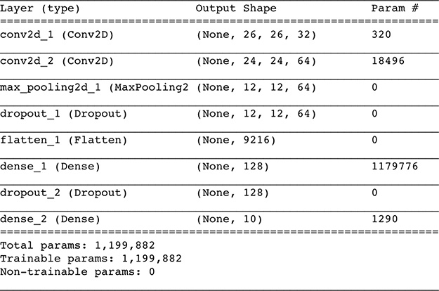
Figure 10.8 A summary of our LeNet-5-inspired ConvNet architecture. Note that the None dimension in each layer is a placeholder for the number of images per batch (i.e., the stochastic gradient descent mini-batch size). Because batch size is specified later (in the model.fit() method), None is used in the interim.
Let’s break down the “Output Shape” column of Figure 10.8 first:
The first convolutional layer,
conv2d_1, takes in the 28×28-pixel MNIST digits. With the chosen kernel hyperparameters (filter size, stride, and padding), the layer outputs a 26×26-pixel activation map (as per Equation 10.3).20 With 32 kernels, the resulting activation map has a depth of 32 slices.The second convolutional layer receives as its input the 26×26×32 activation map from the first convolutional layer. The kernel hyperparameters are unchanged, so the activation map shrinks again, now down to 24 × 24. The map is, however, twice as deep because there are 64 kernels in the layer.
As discussed earlier, a max-pooling layer with a kernel size of 2 and a stride of 2 reduces the volume of data flowing through the network by half in each of the spatial dimensions, yielding an activation map of 12 × 12. The depth of the activation map is not affected by pooling, so it retains 64 slices.
The flatten layer collapses the three-dimensional activation map down to a one-dimensional array with 9,216 elements.21
The dense hidden layer contains 128 neurons, so its output is a one-dimensional array of 128 activation values.
Likewise, the softmax output layer consists of 10 neurons, so it outputs 10 probabilities—one ŷ for each possible MNIST digit.
20.
21. 12 × 12 × 64 = 9,216
Now let’s move on to dissecting the “Param #” column of Figure 10.8:
The first convolutional layer has 320 parameters:
288 weights: 32 filters × 9 weights each (from the 3×3 filter size × 1 channel)
32 biases, one for each filter
The second convolutional layer has 18,496 parameters:
18,432 weights: 64 filters × 9 weights per filter, each receiving input from the 32 filters of the preceding layer
64 biases, one for each filter
The dense hidden layer has 1,179,776 parameters:
1,179,648 weights: 9,216 inputs from the preceding layer’s flattened activation map × 128 neurons in the dense layer22
128 biases, one for each neuron in the dense layer
The output layer has 1,290 parameters:
1,280 weights: 128 inputs from the preceding layer × 10 neurons in the output layer
10 biases, one for each neuron in the output layer
Cumulatively, the entire ConvNet has 1,199,882 parameters, the vast majority (98.3 percent) of which are associated with the dense hidden layer.
To compile the model, we call the model.compile() method as usual. Likewise, the model.fit() method will begin training.23 The results of our best epoch are shown in Figure 10.9. Previously, our best result was attained by Deep Net in Keras—an accuracy of 97.87 percent on the validation set of MNIST digits. But here, the ConvNet inspired by LeNet-5 achieved 99.27 percent validation accuracy. This is fairly remarkable because the CNN wiped away 65.7 percent of the remaining error;24 presumably these now correctly classified instances are some of the trickiest digits to classify because they were not identified correctly by our already solid-performing Deep Net.
![Calculation of epoch is shown. Epoch 9/10 60000/60000 [==============================] negative 39s 654us/step loss: 0.0276 acc: 0.9911 val_loss: 0.0260 val_acc: 0.9927.](http://images-20200215.ebookreading.net/5/4/4/9780135116821/9780135116821__deep-learning-illustrated__9780135116821__graphics__krohn_f10_09.jpg)
Figure 10.9 Our LeNet-5-inspired ConvNet architecture peaked at a 99.27 percent validation accuracy following nine epochs of training, thereby outperforming the accuracy of the dense nets we trained earlier in the book.
22. Notice that the dense layer has two orders of magnitude more parameters than the convolutional layers!
23. These steps are identical to the previous notebooks, with the minor exception that the number of epochs is reduced (to 10), because we found that validation loss stopped decreasing after nine epochs of training.
24. 1 - (100%-99.27%)/(100%-97.87%)
AlexNet and VGGNet in Keras
In our LeNet-inspired architecture (Example 10.3), we included a pair of convolutional layers followed by a max-pooling layer. This is a routine approach within convolutional neural networks. As depicted in Figure 10.10, it is common to group convolutional layers (often one to three of them) together with a pooling layer. These conv-pool blocks can then be repeated several times. As in LeNet-5, such CNN architectures regularly culminate in a dense hidden layer (up to several dense hidden layers) and then the output layer.

Figure 10.10 A general approach to CNN design: A block (shown in red) of convolutional layers (often one to three of them) and a pooling layer is repeated several times. This is followed by one (up to a few) dense layers.
The AlexNet model (Figure 1.17)—which we introduced as the 2012 computer vision competition-winning harbinger of the deep learning revolution—is another architecture that features the convolutional layer block approach provided in Figure 10.10. In our AlexNet in Keras notebook, we use the code shown in Example 10.4 to emulate this structure.25
25. This AlexNet model architecture is the same one visualized by Jason Yosinski with his DeepViz tool. If you didn’t view his video when we mentioned it earlier in this chapter, then we recommend checking it out at bit.ly/DeepViz now.
Example 10.4 CNN model inspired by AlexNet
model = Sequential()

# first conv-pool block:
model.add(Conv2D(96, kernel_size=(11, 11),
          strides=(4, 4), activation='relu',
          input_shape=(224, 224, 3)))
model.add(MaxPooling2D(pool_size=(3, 3), strides=(2, 2)))
model.add(BatchNormalization())

# second conv-pool block:
model.add(Conv2D(256, kernel_size=(5, 5), activation='relu'))
model.add(MaxPooling2D(pool_size=(3, 3), strides=(2, 2)))
model.add(BatchNormalization())

# third conv-pool block:
model.add(Conv2D(256, kernel_size=(3, 3), activation='relu'))
model.add(Conv2D(384, kernel_size=(3, 3), activation='relu'))
model.add(Conv2D(384, kernel_size=(3, 3), activation='relu'))
model.add(MaxPooling2D(pool_size=(3, 3), strides=(2, 2)))
model.add(BatchNormalization())

# dense layers:
model.add(Flatten())
model.add(Dense(4096, activation='tanh'))
model.add(Dropout(0.5))
model.add(Dense(4096, activation='tanh'))
model.add(Dropout(0.5))

# output layer:
model.add(Dense(17, activation='softmax'))
The key points about this particular model architecture are:
For this notebook, we moved beyond the MNIST digits to a dataset of larger-sized (224×224-pixel) images that are full-color (hence the
3channels of depth in theinput_shapeargument passed to the firstConv2Dlayer).AlexNet used larger filter sizes in the earliest convolutional layers relative to what is popular today—for example,
kernel_size=(11, 11).Such use of dropout in only the dense layers near the model output (and not in the earlier convolutional layers) is common. The intuition behind this is that the early convolutional layers enable the model to represent spatial features of images that generalize well beyond the training data. However, a very specific recombination of these features, as facilitated by the dense layers, may be unique to the training dataset and thus may not generalize well to validation data.
![]()
Following AlexNet being crowned the 2012 winner of the ImageNet Large Scale Visual Recognition Challenge, deep learning models suddenly began to be used widely in the competition (see Figure 1.15). Among these models, there has been a general trend toward making the neural networks deeper and deeper. For example, in 2014 the runner-up in the ILSVRC was VGGNet,26 which follows the same repeated conv-pool-block structure as AlexNet; VGGNet simply has more of them, and with smaller (all 3×3-pixel) kernel sizes. We provide the architecture shown in Example 10.5 in our VGGNet in Keras notebook.
26. Developed by the V isual Geometry Group at the University of Oxford: Simonyan, K., and Zisserman, A. (2015). Very deep convolutional networks for large-scale image recognition. arXiv: 1409.1556.
Example 10.5 CNN model inspired by VGGNet
model = Sequential()

model.add(Conv2D(64, 3, activation='relu',
          input_shape=(224, 224, 3)))
model.add(Conv2D(64, 3, activation='relu'))
model.add(MaxPooling2D(2,2))
model.add(BatchNormalization())

model.add(Conv2D(128, 3, activation='relu'))
model.add(Conv2D(128, 3, activation='relu'))
model.add(MaxPooling2D(2,2))
model.add(BatchNormalization())

model.add(Conv2D(256, 3, activation='relu'))
model.add(Conv2D(256, 3, activation='relu'))
model.add(Conv2D(256, 3, activation='relu'))
model.add(MaxPooling2D(2,2))
model.add(BatchNormalization())

model.add(Conv2D(512, 3, activation='relu'))
model.add(Conv2D(512, 3, activation='relu'))
model.add(Conv2D(512, 3, activation='relu'))
model.add(MaxPooling2D(2,2))
model.add(BatchNormalization())

model.add(Conv2D(512, 3, activation='relu'))
model.add(Conv2D(512, 3, activation='relu'))
model.add(Conv2D(512, 3, activation='relu'))
model.add(MaxPooling2D(2,2))
model.add(BatchNormalization())
model.add(Flatten())
model.add(Dense(4096, activation='relu'))
model.add(Dropout(0.5))
model.add(Dense(4096, activation='relu'))
model.add(Dropout(0.5))

model.add(Dense(17, activation='softmax'))
Residual Networks
As our example ConvNets from this chapter (LeNet-5, AlexNet, VGGNet) suggest, there’s a trend over time toward deeper networks. In this section, we recapitulate the topic of vanishing gradients—the (often dramatic) slowing in learning that can occur as network architectures are deepened. We then describe an imaginative solution that has emerged in recent years: residual networks.
Vanishing Gradients: The Bête Noire of Deep CNNs
With more layers, models are able to learn a larger variety of relatively low-level features in the early layers, and increasingly complex abstractions are made possible in the later layers via nonlinear recombination. This approach, however, has limits: If we continue to simply make our networks deeper (e.g., by adding more and more of the conv-pool blocks from Figure 10.10), they will eventually be debilitated by the vanishing gradient problem.
We introduced vanishing gradients in Chapter 9; the basis of the issue is that parameters in early layers of the network are far away from the cost function: the source of the gradient that is propagated backward through the network. As the error is backpropa-gated, a larger and larger number of parameters contribute to the error, and thus each layer closer to the input gets a smaller and smaller update. The net effect is that early layers in increasingly deep networks become more difficult to train (see Figure 8.8).
Because of the vanishing gradient problem, it is commonly observed that as one increases the depth of a network, accuracy increases up to a saturation point and then later begins to degrade as networks become excessively deep. Imagine a shallow network that is performing well. Now let’s copy those layers with their weights, and stack on new layers atop to make the model deeper. Intuition might say that the new, deeper model would take the existing gains from the early pretrained layers and improve. If the new layers performed simple identity mapping (wherein they faithfully reproduced the exact results of the earlier layers), then we’d see no increase in training error. It turns out, however, that plain deep networks struggle to learn identity functions.27,28 Thus, these new layers either add new information and decrease the error, or they do not add new information (but also fail at identity mapping) and the error increases. Given that adding useful information is an exceedingly rare outcome (relative to the baseline, which is essentially random noise), it transpires that beyond a certain point these extra layers will, probabilistically, contribute to an overall degradation in performance.
27. Hardt, M., and Ma, T. (2018). Identity matters in deep learning. arXiv:1611.04231.
28. Hold tight! More clarification is coming up on the terms identity mapping and identity functions shortly.
Residual Connections
Residual networks (or ResNets, for short) rely on the idea of residual connections, which exist within so-called residual modules. A residual module—as illustrated in Figure 10.11—is a collective term for a sequence of convolutions, batch-normalization operations, and ReLU activations that culminates with a residual connection. For the sake of simplicity here, we consider these various layers within a residual module to be a single, discrete unit. Following on with the most straightforward definition, a residual connection exists when the input to one such residual module is summed with its output to produce the final activation for that residual module. In other words, a residual module will receive some input ai–1,29 which is transformed by the convolutions and activation functions within the residual module to generate its output ai. Subsequently, this output and the original input to the residual module are summed: yi = ai + ai–1.30
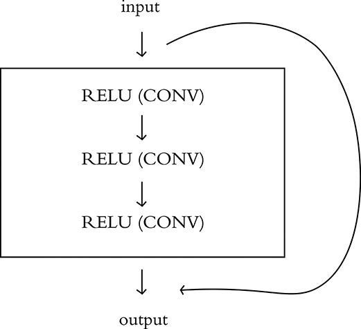
Figure 10.11 A schematic representation of a residual module. Batch normalization and dropout layers are not shown, but may be included.
29. Remember that the input to any given layer is simply the output of the preceding layer, denoted here by ai–1.
30. We’ve opted to denote the final output of the whole residual module as yi, but that does not mean to indicate that this is necessarily the final output of the entire model. It simply serves to avoid confusion with the activations from the current and preceding layers, indicating that the final output is a distinct entity derived from the sum of those activations.
Following the structure and the basic math of the residual connection from the preceding paragraph, you’ll notice that an interesting feature emerges: If the residual module has an activation ai = 0—that is, it has learned nothing—the final output of the residual module will simply be the original input, since the two are summed. Following on with the equation we used most recently:
In this case, the residual module is effectively an identity function. These residual modules either learn something useful and contribute to reducing the error of the network, or they perform identity mapping and do nothing at all. Because of this identity-mapping behavior, residual connections are also called “skip connections,” because they enable information to skip the functions located within the residual module.
In addition to this neutral-or-better characteristic of residual networks, we should also highlight the value of their inherent multiplicity. Consider the schematic in Figure 10.12: When several residual modules are stacked, later residual modules receive inputs that are increasingly complex combinations of the residual modules and skip connections from earlier in the network. Seen on the right in this figure, a decision tree representation shows how, at each of the three residual modules in the network, information may either pass through the residual block or bypass it via a skip connection. Thus, as is shown at the bottom of the figure, with only three residual modules there are eight possible paths the information can take. In practice, the process is not commonly as binary as it is depicted in this figure. That is, the value of ai is seldom 0, and therefore the output is usually some mix of the identity function and the residual module. Given this insight, residual networks can be thought of as complex combinations or ensembles of many shallower networks that are pooled at various depths.

Figure 10.12 Shown at left is the conventional representation of residual blocks within a residual network. Shown at right is an unraveled view, which demonstrates how, depending on which skip connections are used, the final path of information from input to output can be varied by the network.
ResNet
The first deep residual network, ResNet, was introduced by Microsoft Research in 201531 and won first place in that year’s ILSVRC image-classification competition. Referring back to Figure 1.15, this makes ResNet the leader of the pack of deep learning algorithms that surpassed human performance at image recognition in 2015.
31. He, K., et al. (2015). Deep residual learning for image recognition. arXiv:1512.03385.
Up to this point in the book, we’ve made it sound as if image classification is the only contest at ILSVRC, but in fact ILSVRC has several machine vision competition categories, such as object detection and image segmentation (more on these two machine vision tasks coming soon in this chapter). In 2015, ResNet took first place not only in the ILSVRC image-classification competition but in the object detection and image segmentation categories, too. Further, in the same year, ResNet was also recognized as champion of the detection and segmentation competitions involving an alternative image dataset called COCO, which is an alternative to the ILSVRC set.32
Given the broad sweep of machine vision trophies upon the invention of residual networks, it’s clear they were a transformative innovation. They managed to squeeze out more juice relative to the existing networks by enabling much deeper architectures without the decrease in performance associated with those extra layers if they fail to learn useful information about the problem.
In this book, we strive to make our code examples accessible to our readers by having model architectures and datasets that are small enough to carry out training on even a modest laptop computer. Residual network architectures, as well as the datasets that make them worthwhile, do not fall into this category. That said, using a powerful, general approach called transfer learning—which we will introduce at the end of this chapter—we provide you with resources to nevertheless take advantage of very deep architectures like ResNet with the model’s parameters pretrained on massive datasets.
Applications of Machine Vision
In this chapter, you’ve learned about layer types that enable machine vision models to perform well. We’ve also discussed some of the approaches that are used to improve these models, and we’ve delved into some of the canonical machine vision algorithms of the past few years. Up to here in the chapter, we’ve dealt with the problem of image classification—that is, identifying the main subject in an image, as seen at the left in Figure 10.13. Now, to wrap up the chapter, we turn our focus to other interesting applications of machine vision beyond image classification. The first is object detection, seen in the second panel from the left in Figure 10.13, wherein the algorithm is tasked with drawing bounding boxes around objects in an image. Next is image segmentation, shown in the third and fourth panels of Figure 10.13. Semantic segmentation identifies all objects of a particular class down to the pixel level, whereas instance segmentation discriminates between different instances of a particular class, also at the pixel level.

Figure 10.13 These are examples of various machine vision applications. We have encountered classification previously in this chapter, but now we cover object detection, semantic segmentation, and instance segmentation.
Object Detection
Imagine a photo of a group of people sitting down to dinner. There are several people in the image. There is a roast chicken in the middle of the table, and maybe a bottle of wine. If we desired an automated system that could predict what was served for dinner or to identify the people sitting at the table, an image-classification algorithm would not provide that level of granularity—enter object detection.
Object detection has broad applications, such as detecting pedestrians in the field of view for autonomous driving, or for identifying anomalies in medical images. Generally speaking, object detection is divided into two tasks: detection (identifying where the objects in the image are) and then, subsequently, classification (identifying what the objects are that have been detected). Typically this pipeline has three stages:
A region of interest must be identified.
Automatic feature extraction is performed on this region.
The region is classified.
Seminal models—ones that have defined progress in this area—include R-CNN, Fast R-CNN, Faster R-CNN, and YOLO.
R-CNN
R-CNN was proposed in 2013 by Ross Girshick and his colleagues at UC Berkeley.33 The algorithm was modeled on the attention mechanism of the human brain, wherein an entire scene is scanned and focus is placed on specific regions of interest. To emulate this attention, Girshick and his coworkers developed R-CNN to:
Perform a selective search for regions of interest (ROIs) within the image.
Extract features from these ROIs by using a CNN.
Combine two “traditional” (as in Figure 1.12) machine learning approaches—called linear regression and support vector machines—to, respectively, refine the locations of bounding boxes34 and classify objects within each of those boxes.
33. Girshnick, R., et al. (2013). Rich feature hierarchies for accurate object detection and semantic segmentation. arXiv: 1311.2524.
34. See examples of bounding boxes in Figure 10.14.
R-CNNs redefined the state of the art in object detection, achieving a massive gain in performance over the previous best model in the Pattern Analysis, Statistical Modeling and Computational Learning (PASCAL) Visual Object Classes (VOC) competition.35 This ushered in the era of deep learning in object detection. However, this model had some limitations:
It was inflexible: The input size was fixed to a single specific image shape.
It was slow and computionally expensive: Both training and inference are multistage processes involving CNNs, linear regression models, and support vector machines.
35. PASCAL VOC ran competitions from 2005 until 2012; the dataset remains available and is considered one of the gold standards for object-detection problems.
Fast R-CNN
To address the primary drawback of R-CNN—its speed—Girshick went on to develop Fast R-CNN.36 The chief innovation here was the realization that during step 2 of the R-CNN algorithm, the CNN was unnecessarily being run multiple times, once for each region of interest. With Fast R-CNN, the ROI search (step 1) is run as before, but during step 2, the CNN is given a single global look at the image, and the extracted features are used for all ROIs simultaneously. A vector of features is extracted from the final layer of the CNN, which (for step 3) is then fed into a dense network along with the ROI. This dense net learns to focus on only the features that apply to each individual ROI, culminating in two outputs per ROI:
A softmax probability output over the classification categories (for a prediction of what class the detected object belongs to)
A bounding box regressor (for refinement of the ROI’s location)
36. Girshnick, R. (2015). Fast R-CNN. arXiv: 1504.08083
Following this approach, the Fast R-CNN model has to perform feature extraction using a CNN only once for a given image (thereby reducing computational complexity), and then the ROI search and dense layers work together to finish the object-detection task. As the name suggests, the reduced computational complexity of Fast R-CNN corresponds to speedier compute times. It also represents a single, unified model without the multiple independent parts of its predecessor. Nevertheless, as with R-CNN, the initial (ROI search) step of Fast R-CNN still presents a significant computational bottleneck.
Faster R-CNN
The model architectures in this section are clever works of innovation—their names, however, are not. Our third object-detection algorithm of note is Faster R-CNN, which (you guessed it!) is even swifter than Fast R-CNN.
Faster R-CNN was revealed in 2015 by Shaoqing Ren and his coworkers at Microsoft Research (Figure 10.14 shows example outputs).37 To overcome the ROI-search bottleneck of R-CNN and Fast R-CNN, Ren and his colleagues had the cunning insight to leverage the feature activation maps from the model’s CNN for this step, too. Those activation maps contain a great deal of contextual information about an image. Because each map has two dimensions representing location, they can be thought of as literal maps of the locations of features within a given image. If—as in Figure 10.6—a convolutional layer has 16 filters, the activation map it outputs has 16 maps, together representing the locations of 16 features in the input image. As such, these feature maps contain rich detail about what is in an image and where it is. Faster R-CNN takes advantage of this rich detail to propose ROI locations, enabling a CNN to seamlessly perform all three steps of the object-detection process, thereby providing a unified model architecture that builds on R-CNN and Fast R-CNN but is markedly quicker.

Figure 10.14 These are examples of object detection (performed on four separate images by the Faster R-CNN algorithm). Within each region of interest—defined by the bounding boxes within the images—the algorithm predicts what the object within the region is.
37. Ren, S. et al. (2015). Faster R-CNN: Towards real-time object detection with region proposal networks. arXiv: 1506.01497.
YOLO
Within each of the various object-detection models described thus far, the CNN focused on the individual proposed ROIs as opposed to the whole input image.38 Joseph Redmon and coworkers published on You Only Look Once (YOLO) in 2015, which bucked this trend.39 YOLO begins with a pretrained40 CNN for feature extraction. Next, the image is divided into a series of cells, and, for each cell, a number of bounding boxes and object-classification probabilities are predicted. Bounding boxes with class probabilities above a threshold value are selected, and these combine to locate an object within an image.
38. Technically, the CNN looked at the whole image at the start in both Fast R-CNN and Faster R-CNN. However, in both cases this was simply a one-shot step to extract features, and from then onward the image was treated as a set of smaller regions.
39. Redmon, J., et al. (2015). You Only Look Once: Unified, real-time object detection. arXiv: 1506.02640.
40. Pretrained models are used in transfer learning, which we detail at chapter’s end.
You can think of the YOLO method as aggregating many smaller bounding boxes, but only if they have a reasonably good probability of containing any given object class. The algorithm improved on the speed of Faster R-CNN, but it struggled to accurately detect small objects in an image.
Since the original YOLO paper, Redmon and his colleagues have released their YOLO900041 and YOLOv3 models.42 YOLO9000 resulted in increases in both execution speed and model accuracy, and YOLOv3 yielded some speed for even further improved accuracy—in large part due to the increased sophistication of the underlying model architectures. The details of these continuations stretch beyond the scope of this book, but at the time of writing these models represent the cutting edge of object-detection algorithms.
41. Redmon,J., et al. (2016). YOLO9000: Better, faster, stronger. arXiv: 1612.08242.
42. Redmon,J. (2018). YOLOv3: An incremental improvement. arXiv: 1804.02767.
Image Segmentation
When the visual field of a human is exposed to a real-world scene containing many overlapping visual elements—such as the game of association football (soccer) captured in Figure 10.15—the adult brain seems to effortlessly distinguish figures from the background, defining the boundaries of these figures and relationships between them within a few hundred milliseconds. In this section, we cover image segmentation, another application area where deep learning has in a few short years bridged much of the gap in visual capability between humans and machines. We focus on two prominent model architectures—Mask R-CNN and U-Net—that are able to reliably classify objects in an image on a pixelwise scale.
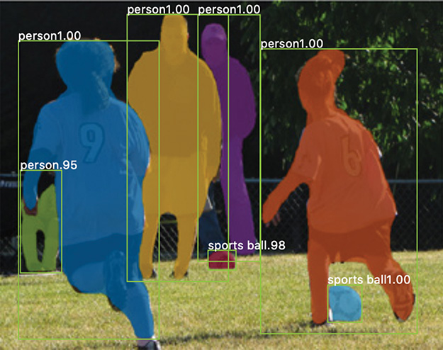
Figure 10.15 This is an example of image segmentation (as performed by the Mask R-CNN algorithm). Whereas object detection involves defining object locations with coarse bounding boxes, image segmentation predicts the location of objections to the pixel level.
Mask R-CNN
Mask R-CNN was developed by Facebook AI Research (FAIR) in 2017.43 This approach involves:
Using the existing Faster R-CNN architecture to propose ROIs within the image that are likely to contain objects.
An ROI classifier predicting what kind of object exists in the bounding box while also refining the location and size of the bounding box.
Using the bounding box to grab the parts of the feature maps from the underlying CNN that correspond to that part of the image.
Feeding the feature maps for each ROI into a fully convolutional network that outputs a mask indicating which pixels correspond to the object in the image. An example of such a mask—consisting of bright colors to designate the pixels associated with separate objects—is provided in Figure 10.15.
43. He, K., et al. (2017). Mask R-CNN. arXiv: 1703.06870.
Image segmentation problems require binary masks as labels for training. These consist of arrays of the same dimensions as the original image. However, instead of RGB pixel values they contain 1s and 0s indicating where in the image the object is, with the 1s representing a given object’s pixel-by-pixel location (and the 0s representing everywhere else). If an image contains a dozen different objects, then it must have a dozen binary masks.
U-Net
Another popular image segmentation model is U-Net, which was developed at the University of Freiberg (and was mentioned at the end of Chapter 3 with respect to the automated photo-processing pipelines).44 U-Net was created for the purpose of segmenting biomedical images, and at the time of writing it outperformed the best available methods in two challenges held by the International Symposium on Biomedical Images.45
44. Ronneberger, O., et al. (2015). U-Net: Convolutional networks for biomedical image segmentation. arXiv: 1505.04597.
45. The two challenges were the segmentation of neuronal structures in electron microscopy stacks, and the ISBI cell-tracking challenge from 2015.
The U-Net model consists of a fully convolutional architecture, which begins with a contracting path that produces successively smaller and deeper activation maps through multiple convolution and max-pooling steps. Subsequently, an expanding path restores these deep activation maps back to full resolution through multiple upsampling and convolution steps. These two paths—the contracting and expanding paths—are symmetrical (forming a “U” shape), and because of this symmetry the activation maps from the contracting path can be concatenated onto those of the expanding path.
The contracting path serves to allow the model to learn high-resolution features from the image. These high-res features are handed directly to the expanding path. By the end of the expanding path, we expect the model to have localized these features within the final image dimensions. After concatenating the feature maps from the contracting path onto the expanding path, a subsequent convolutional layer allows the network to learn to assemble and localize these features precisely. The final result is a network that is highly adept both at identifying features and at locating those features within two-dimensional space.
Transfer Learning
To be effective, many of the models we describe in this chapter are trained on very large datasets of diverse images. This training requires significant compute resources, and the datasets themselves are not cheap or easy to assemble. Over the course of this training, a given CNN learns to extract general features from the images. At a low level, these are lines, edges, colors, and simple shapes; at a higher level, they are textures, combinations of shapes, parts of objects, and other complex visual elements (recall Figure 1.17). If the CNN has been trained on a suitably varied set of images and if it is sufficiently deep, these feature maps likely contain a rich library of visual elements that can be assembled and combined to form nearly any image. For example, a feature map that identifies a dimpled texture combined with another that recognizes round objects and yet another that responds to white colors could be recombined to correctly identify a golf ball. Transfer learning takes advantage of this library of existing visual elements contained within the feature maps of a pretrained CNN and repurposes them to become specialized in identifying new classes of objects.
Say, for example, that you’d like to build a machine vision model that performs the binary classification task we’ve addressed time and again since Chapter 6: distinguishing hot dogs from anything that is not a hot dog. Of course, you could design a large and complex CNN that takes in images of hot dogs and, well . . . not hot dogs, and outputs a single sigmoid class prediction. You could train this model on a large number of training images, and you’d expect the convolutional layers early in the network to learn a set of feature maps that will identify hot dog-esque features. Frankly, this would work pretty well. However, you’d need a lot of time and a lot of compute power to train the CNN properly, and you’d need a large number of diverse images so that the CNN could learn a suitably diverse set of feature maps. This is where transfer learning comes in: Instead of training a model from scratch, you can leverage the power of a deep model that has already been trained on a large set of images and quickly repurpose it to detecting hot dogs specifically.
Earlier in this chapter, we mentioned VGGNet as an example of a classic machine vision model architecture. In Example 10.5 and in our VGGNet in Keras Jupyter notebook, we showcase the VGGNet16 model, which is composed of 16 layers of artificial neurons—mostly repeating conv-pool blocks (see Figure 10.10). The closely related VGGNet19 model, which incorporates one further conv-pool block (containing three convolutional layers), is our pick for our transfer-learning starting point. In our accompanying notebook, Transfer Learning in Keras, we load VGGNet19 and modify it for our own hot-doggy purposes.
![]()
To start, let’s get the standard imports out of the way and load up the pretrained VGGNet19 model (Example 10.6).
Example 10.6 Loading the VGGNet19 model for transfer learning
# Load dependencies:
from keras.applications.vgg19 import VGG19
from keras.models import sequential
from keras.layers import Dense, Dropout, Flatten
from keras.preprocessing.image import ImageDataGenerator

# Load the pre-trained VGG19 model:
vgg19 = VGG19(include_top=False,
              weights='imagenet',
              input_shape=(224,224, 3),
              pooling=None)

# Freeze all the layers in the base VGGNet19 model:
for layer in vgg19.layers:
    layer.trainable = False
Handily, Keras provides the network architecture and parameters (called weights, but includes biases, too) already, so loading the pretrained model is easy.46 Arguments passed to the VGG19 function help to define some characteristics of the loaded model:
46. For other pretrained Keras models, including the ResNet architecture we introduced earlier in this chapter, visit keras.io/applications.
include_top=Falsespecifies that we do not want the final dense classification layers from the original VGGNet19 architecture. These layers were trained for classifying the original ImageNet data. Rather, as you’ll see momentarily, we’ll make our own top layers and train them ourselves using our own data.weights='imagenet'is to load model parameters trained on the 14 million-sample ImageNet dataset.47input_shape=(224,224,3)initializes the model with the correct input image size to handle our hot dog data.
47. The only other weights argument option at the time of writing is 'None', which would be a random initialization, but in the future, model parameters trained on other datasets could be available.
After we load the model, a quick for loop traverses each layer in the model and sets its trainable flag to False so that the parameters in these layers will not be updated during training. We are confident that the convolutional layers of VGGNet19 have been effectively trained to represent the generalized visual-imagery features of the large ImageNet dataset, so we leave the base model intact.
In Example 10.7, we add fresh dense layers on top of the base VGGNet19 model. These layers take the features extracted from the input image by the pretrained convolutional layers, and through training they will learn to use these features to classify the images as hot dogs or not hot dogs.
Example 10.7 Adding classification layers to transfer-learning model
# Instantiate the sequential model and add the VGG19 model:
model = Sequential()
model.add(vgg19)

# Add the custom layers atop the VGG19 model:
model.add(Flatten(name='flattened'))
model.add(Dropout(0.5, name='dropout'))
model.add(Dense(2, activation='softmax', name='predictions'))

# Compile the model for training:
model.compile(optimizer='adam', loss='categorical_crossentropy',
              metrics=['accuracy'])
Next, we use an instance of the ImageDataGenerator class to load the data (Example 10.8). This class is provided by Keras and serves to load images on the fly. It’s especially helpful if you don’t want to load all of your training data into memory right away, or when you might want to perform random data augmentations in real time during training.48
48. In Chapter 9, we mention that data augmentation is an effective way to increase the size of a training dataset, thereby helping a model generalize to previously unseen data.
Example 10.8 Defining data generators
# Instantiate two image generator classes:
train_datagen = ImageDataGenerator(
    rescale=1.0/255,
    data_format='channels_last',
    rotation_range=30,
    horizontal_flip=True,
    fill_mode='reflect')
valid_datagen = ImageDataGenerator(
    rescale=1.0/255,
    data_format='channels_last')

# Define the batch size:
batch_size=32

# Define the train and validation data generators:
train_generator = train_datagen.flow_from_directory(
    directory='./hot-dog-not-hot-dog/train',
    target_size=(224, 224),
    classes=['hot_dog','not_hot_dog'],
    class_mode='categorical',
    batch_size=batch_size,
    shuffle=True,
    seed=42)

valid_generator = valid_datagen.flow_from_directory(
    directory='./hot-dog-not-hot-dog/test',
    target_size=(224, 224),
    classes=['hot_dog','not_hot_dog'],
    class_mode='categorical',
    batch_size=batch_size,
    shuffle=True,
    seed=42)
The train-data generator will randomly rotate the images within a 30-degree range, randomly flip the images horizontally, rescale the data to between 0 and 1 (by multiplying by 1/255), and load the image data into arrays in the “channels last” format.49 The validation generator only needs to rescale and load the images; data augmentation would be of no value there. Finally, the flow_from_directory() method directs each generator to load the images from a directory we specify.50 The remainder of the arguments to this method should be intuitive.
49. Look back at Example 10.6, and you’ll see that the model accepts inputs with dimensions of 224 × 224 × 3—that is, the channels dimension is last. The alternative is to set up the color channel as the first dimension.
50. Instructions for downloading the data are included in our Jupyter notebook.
Now we’re ready to train (Example 10.9). Instead of using the fit() method as we did in all previous cases of model-fitting in this book, here we call the fit_generator() method on the model because we’ll be passing in a data generator in place of arrays of data.51 During our run of this model, our best epoch turned out to be the sixth, in which we attained 81.2 percent accuracy.
51. As we warned earlier in this chapter, in the section on AlexNet and VGGNet, with very large models you may encounter out-of-memory errors. Please refer to bit.ly/DockerMem for information on increasing the amount of memory available to your Docker container. Alternatively, you could reduce your batch-size hyperparameter.
Example 10.9 Train transfer-learning model
model.fit_generator(train_generator, steps_per_epoch=15,
                    epochs=16, validation_data=valid_generator,
                    validation_steps=15)
This demonstrates the power of transfer learning. With a small amount of training and almost no time spent on architectural considerations or hyperparameter tuning, we have at our fingertips a model that performs reasonably well on a rather complicated image-classification task: hot dog identification. With some time invested in hyperparameter tuning, the results could be improved further.
Capsule Networks
In 2017, Sara Sabour and her colleagues on Geoff Hinton’s (Figure 1.16) Google Brain team in Toronto made a splash with a novel concept called capsule networks.52 Capsule networks have received considerable interest, because they are able to take positional information into consideration. CNNs, to their great detriment, do not; so a CNN would, for example, consider both of the images in Figure 10.16 to be a human face. The theory behind capsule networks is beyond the scope of this book, but machine vision practitioners are generally aware of them so we wanted to be sure you were, too. Today, they are too computationally intensive to be predominant in applications, but cheaper compute and theoretical advancements could mean that this situation will change soon.
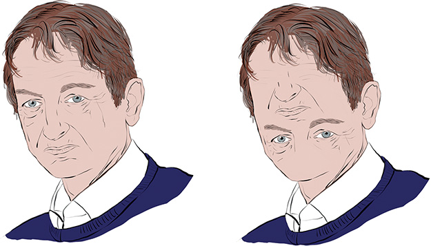
Figure 10.16 With convolutional neural networks, which are agnostic to the relative positioning of image features, the figure on the left and the one on the right are equally likely to be classified as Geoff Hinton’s face. Capsule networks, in contrast, take positional information into consideration, and so would be less likely to mistake the right-hand figure for a face.
52. Sabour, S., et al. (2017). Dynamic routing between capsules. arXiv: 1710.09829.
Summary
In this chapter, you learned about convolutional layers, which are specialized to detect spatial patterns, making them particularly useful for machine vision tasks. You incorporated these layers into a CNN inspired by the classic LeNet-5 architecture, enabling you to surpass the handwritten-digit recognition accuracy of the dense networks you designed in Part II. The chapter concluded by discussing best practices for building CNNs and surveying the most noteworthy applications of machine vision algorithms. In the coming chapter, you’ll discover that the spatial-pattern recognition capabilities of convolutional layers are well suited not only to machine vision but also to other tasks.
Key Concepts
Here are the essential foundational concepts thus far. New terms from the current chapter are highlighted in purple.
parameters:
weight w
bias b
activation a
artificial neurons:
sigmoid
tanh
ReLU
linear
input layer
hidden layer
output layer
layer types:
dense (fully connected)
softmax
convolutional
max-pooling
flatten
cost (loss) functions:
quadratic (mean squared error)
cross-entropy
forward propagation
backpropagation
unstable (especially vanishing) gradients
Glorot weight initialization
batch normalization
dropout
optimizers:
stochastic gradient descent
Adam
optimizer hyperparameters:
learning rate η
batch size