14. Moving Forward with Your Own Deep Learning Projects
Congratulations, you’ve made it to the closing chapter of the book! In Part I, we introduced deep learning: what it is and how it has become predominant. In Part II, we delved into the essential theory of deep learning. And in Part III, we applied the theory you learned to a broad range of problems spanning vision, language, art, and changing environments.
In this chapter, we provide you with resources and advice for moving onward from the examples provided in Part III to your very own deep learning projects, some of which could be of tremendous benefit to society. We cap everything off by providing context on how your work may contribute to deep learning’s ongoing overhaul of software globally and perhaps even to the dawn of artificial general intelligence.
Ideas for Deep Learning Projects
In this section, we cover candidate ideas for your own first deep learning projects.
Machine Vision and GANs
The easiest way to get your feet wet with a deep learning problem of your own might be to load up the Fashion-MNIST dataset.1 Keras comes preloaded with these data, which consist of 10 classes of photos of clothing (see Table 14.1). The Fashion-MNIST data have identical dimensions to the handwritten MNIST digits you familiarized yourself with in Part II: They are 8-bit 28×28-pixel grayscale bitmaps (an example is provided in Figure 14.1) spread across 60,000 training-image and 10,000 validation-image sets. Thus, by replacing the data-loading line (e.g., Example 5.2) of any existing MNIST-classifying Jupyter notebook from this book with the following code, the Fashion-MNIST data can trivially be substituted in:
from keras.datasets import fashion_mnist
(X_train, y_train), (X_valid, y_valid) = fashion_mnist.load_data()

Figure 14.1 Following our pixel-by-pixel rendering of an MNIST digit (Figure 5.3), this is an example of an image from the Fashion-MNIST dataset. This particular image belongs to class 9, so—as per Table 14.1—it is an ankle boot. Check out our Fashion MNIST Pixel by Pixel Jupyter notebook for the code we used to create this figure.
Table 14.1 Fashion-MNIST categories
Class |
Label Description |
|---|---|
0 |
t-shirt |
1 |
trousers |
2 |
pullover |
3 |
dress |
4 |
coat |
5 |
sandal |
6 |
shirt |
7 |
sneaker |
8 |
bag |
9 |
ankle boot |
1. Xiao, H., et al. (2017). Fashion-MNIST: A novel image dataset for benchmarking machine learning algorithms. arXiv: 1708.07747.
From there, you can begin experimenting with modifying your model architecture and tuning your hyperparameters to improve validation-set accuracy. The Fashion-MNIST data are quite a bit more challenging to classify relative to the handwritten MNIST digits, so they present a rewarding problem for applying the material you learned in this book. By Chapter 10, we observed greater than 99 percent validation accuracy with MNIST (see Figure 10.9), but obtaining validation accuracy greater than 92 percent with Fashion-MNIST is not easy, and achieving anything greater than 94 percent is downright impressive.
Other excellent machine vision datasets for deep learning image-classification models can be found via the following sources:
Kaggle: This data-science competition platform has many real-world datasets. Building a winning model could earn you real-world money, too! For example, the platform’s Cdiscount Image Classification Challenge had a $35,000 cash prize for classifying images of products for a French e-commerce giant.2 The datasets available via Kaggle come and go as competitions begin and end, but at any given time there are likely to be a number of large image datasets available—with model-building experience, kudos, and maybe even cash prizes for you to benefit from.
Figure Eight: This data-labeling-via-crowdsourcing company (formerly known as CrowdFlower) provides dozens of publicly available, superbly curated image-classification datasets. To peruse what’s available, visit figure-eight.com/data-for-everyone and search for the word image.
The researcher Luke de Oliveira compiled a clear, concise list of the best-known datasets among deep learning practitioners. Have a look under the “Computer Vision” heading at
bit.ly/LukeData.
2. bit.ly/kaggleCD
If you’re looking to build and tune your own GAN, small datasets you could start off with include:
One or more of the classes of images from the Quick, Draw! dataset we leveraged in Chapter 123
The Fashion-MNIST data
The plain old handwritten MNIST digits
Natural Language Processing
In the same way that the Fashion-MNIST data plug right in to the image-classification models we built in this book, datasets curated by Xiang Zhang and his colleagues from Yann LeCun’s (Figure 1.9) lab can be dropped straightforwardly into the natural-language-classification models we built in Chapter 11, making them ideal data for a first NLP project of your own.
All eight of Zhang et al.’s natural language datasets are described in detail in their paper4 and are available for download at bit.ly/NLPdata. Each dataset is at least an order of magnitude larger than the 25,000-training-sample IMDb film-sentiment data we worked with in Chapter 11, enabling you to experiment with the value of much more complex deep learning models and much richer word-vector spaces. Six of the datasets have more than two classes (which would require you to have multiple output neurons in a softmax layer), and the other two are binary classification problems (enabling you to retain the single sigmoid output we used for the IMDb data):
4. See section four (“Large-scale Datasets and Results”) of Zhang, X., et al. (2016). Character-level convolutional networks for text classification. arXiv: 1509.01626.
Yelp Review Polarity: 560,000 training samples and 38,000 validation samples that are classed as either positive (four- or five-star) or negative (one- or two-star) reviews of services and locations posted on the website Yelp
Amazon Review Polarity: A whopping 3.6 million training samples and 400,000 validation samples collected from the e-retail giant Amazon that are either positive or negative product reviews
As with machine vision, NLP data available from Kaggle, Figure Eight (again, search for the word sentiment or text on figure-eight.com/data-for-everyone), and Luke de Oliveira (under the “Natural Language” heading at bit.ly/LukeData) would form the basis of solid self-directed deep learning projects.
Deep Reinforcement Learning
A first deep reinforcement learning project could involve a:
New environment: By changing the OpenAI Gym environment in our Cartpole DQN notebook,5 you can use the DQN agent you studied in Chapter 13 to tackle an environment other than the Cart-Pole game. Some relatively simple options include Mountain Car (
MountainCar-v0) and Frozen Lake (FrozenLake-v0).New agent: If you have access to a Unix-based machine (which includes ones running macOS), you can install SLM Lab (Figure 13.10) to try out other agents (e.g., an Actor-Critic agent; see Figure 13.12). Some of these could be sophisticated enough to excel in advanced environments like the Atari games6 provided by OpenAI Gym or the three-dimensional environments provided by Unity.
5. To do this, change the string argument you pass into gym.make() from Example 13.1.
Once you’re comfortable with fairly advanced agents, it could be rewarding to try them out in other environments like DeepMind Lab (Figure 4.14) or to unleash a single agent upon multiple different environments simultaneously (SLM Lab can help facilitate this for you).
Converting an Existing Machine Learning Project
Although all of the projects we’ve suggested thus far involve using third-party data sources, you may very well have collected data already yourself. You may even have already used these data for machine learning—say, with a linear regression model or support vector machines. In these cases, you could feed the data you already have into a deep learning model. You could begin with a three-hidden-layer dense net like our Deep Net in Keras model from Chapter 9. If you’re keen to predict a continuous variable as opposed to a categorical one, then perhaps our Regression in Keras notebook (covered near the end of Chapter 9) would serve as an appropriate template.
You could feed more or less unadulterated data into your deep learning model, or, if you’ve already extracted features from your raw data, there’s certainly no harm in passing these features in as inputs. Indeed, researchers from Google7 have popularized a wide and deep modeling approach that handles existing engineered features while simultaneously learning new features from raw input data. See Figure 14.2 for a generalized schematic of this wide and deep approach, which incorporates the concat layer introduced at the end of Chapter 11 (see Example 11.41).
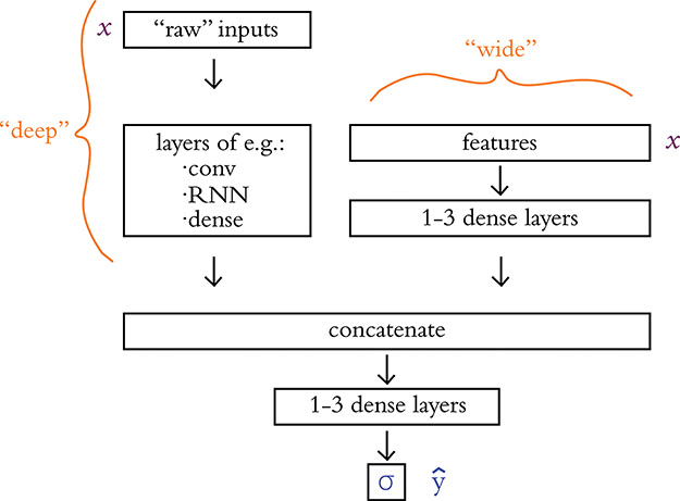
Figure 14.2 The wide and deep model architecture concatenates together inputs from two separate legs. The deep leg receives more or less unadulterated (“raw”) input data and uses several data-appropriate (e.g., convolutional, recurrent, dense) layers of neurons to extract features automatically. Its “deep”-ness may result from having many layers of neurons. The wide leg, meanwhile, receives manually curated features (extracted from the raw data prior to modeling via expertly defined functions) as inputs. Its “wide”-ness may result from having many such features serving as inputs.
7. bit.ly/wideNdeep
Resources for Further Projects
For moving beyond the initial projects suggested above, we maintain a directory of helpful resources at jonkrohn.com/resources. There, we provide links to:
Open data sources that are well organized and, in many cases, very large
Recommended hardware and cloud infrastructure options for training larger deep learning models
Compilations of key deep learning papers and implementations of the research covered within them
Interactive deep learning demos
Examples of recurrent neural networks applied to times series predictions, such as financial applications8
8. This topic is of great interest to many students of deep learning, but it’s beyond the scope of this book.
Socially Beneficial Projects
In particular, we’d like to draw your attention to the section of our resources page titled “Problems Worth Solving.” In this section, we list resources that summarize the most pressing global issues facing society in our time—issues that we encourage you to apply deep learning techniques toward solving. As an example, in one of these studies,9 the authors—from the McKinsey Global Institute—examine 10 social-impact domains:
Equality and inclusion
Education
Health and hunger
Security and justice
Information verification and validation
Crisis response
Economic empowerment
Public and social sector
The environment
Infrastructure
9. Chui, M. (2018). Notes from the AI frontier: Applying AI for social good. McKinsey Global Institute.bit.ly/aiForGood
They go on to detail the prospective utility of many of the techniques introduced in this book to each of these domains, including the following particular examples:
Deep learning on structured data (the dense nets of Chapters 5 to 9): applicable to all 10 domains
Image classification, including handwriting recognition (Chapter 10): all domains except public and social sector
NLP, including sentiment analysis (Chapter 11): all domains except infrastructure
Content generation (Chapter 12): applicable to the equality and inclusion domain as well as to the public and social sector domain
Reinforcement learning (Chapter 13): applicable to the health and hunger domain
The Modeling Process, Including Hyperparameter Tuning
With any of the deep learning project ideas we’ve covered in this chapter, hyperparameter tuning is likely to prove key to your success. In this section, we provide you with a step-by-step modeling process that you can use as a rough template for your own projects. Bear in mind, however, that you may need to stray from our recommended procedural path in a number of ways because of the unique specifics of your particular project. For example, you’re unlikely to proceed strictly linearly through the following steps: As you reach later steps in the process, you may develop a hunch10 about how an earlier step might be improved based on model behavior,11 so you’ll end up circling back and proceeding through some of the steps several times—perhaps even dozens of times or more!
![]()
10. As you carry out more and more of your own deep learning projects, and as you examine more and more of other people’s high-performing model architectures (e.g., in GitHub, StackOverflow, and arXiv papers), you’ll develop an intuition for how to adapt your model’s design and hyperparameters to a given problem.
11. Model behavior can be studied by, for example, monitoring training- and validation-set loss as your model trains. This would be made easier by using TensorBoard (see Figure 9.8).
Here’s our rough step-by-step guide:
Parameter initialization: As covered in Chapter 9 (see Figure 9.3), you should initialize your model’s parameters with sensible random values. We recommend initializing biases with zeros and initializing weights using Xavier Glorot’s approach. Thankfully, with Keras, sensible layer initializations such as these will generally be handled for you automatically.
Cost function selection: If you’re solving a classification problem, you should probably be using cross-entropy cost. If you’re solving a regression problem, then you should probably be using mean-squared-error cost. If you’re interested in experimenting, however,
keras.io/lossesoffers further options.Get above chance: If your initial model architecture (which could be based directly on any of the models we went over in this book) attains below-chance performance on your validation data (e.g., <10 percent accuracy with the 10-class MNIST-digit data) then consider these tactics.
Simplifying your problem: For example, if you’re working with the MNIST digits, you could reduce the number of classes you’re classifying from 10 down to 2.
Simplifying your network architecture: Perhaps you’re doing something rather silly and not realizing it. Or perhaps your model is too deep and your gradient of learning is vanishing severely. By simplifying your model architecture—such as by removing layers—you may bring these potential issues to light.
Reducing your training set size: If you have a large training dataset, waiting for a single epoch to finish training could take a long time. By drastically subsetting your training sample, you can iterate and improve your model more rapidly.
Layers: Once your model is learning to any extent, you can begin experimenting with your layers. You could try:
Varying the number of layers: Following the guidelines discussed in Chapter 8 (the section containing Figure 8.8), you could try adding or removing individual layers or blocks of layers (like the conv-pool blocks in Figure 10.10).
Varying the types of layers: Depending on your particular problem and dataset, particular layer types might markedly outperform others. Consider, for example, the impact of the layer changes we made across our film-sentiment classifiers in Chapter 11 (see Table 11.6 for a summary).
Varying layer width: We recommend varying the number of neurons per layer by powers of 2, also as per Chapter 8 near Figure 8.8.
Avoid overfitting: As discussed in Chapter 9, we recommend encouraging your model to generalize beyond your training dataset by employing dropout, data augmentation (if possible, e.g., with image data), and/or batch normalization. If you happen to be able to acquire additional, new training data for your model, that would likely be helpful, too. Finally, as we demonstrated countless times in Chapter 11, if your model does overfit during training, it’d be wise to reload the model weights from a previous epoch—probably the one in which the validation loss was lowest (see Figure 14.3 for an example).
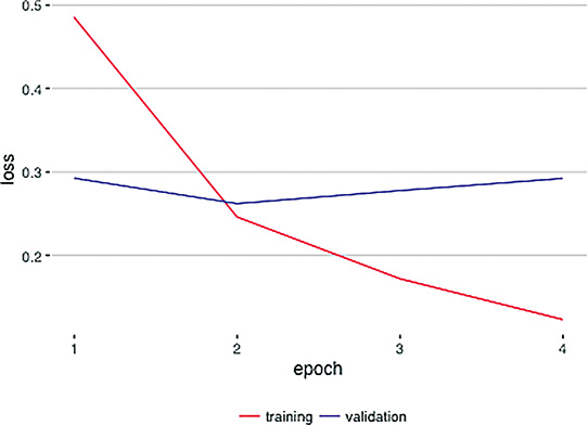
Figure 14.3 A plot of training loss (red) and validation loss (blue) over epochs of model training. These particular results come from our Multi ConvNet Sentiment Classifier notebook (see the final section of Chapter 11), but this overfitting pattern is typical of deep learning models. After epoch 2, the training loss continues toward zero while the validation loss creeps upward. Epoch 2 has the lowest validation loss, so the parameters from that epoch should be reloaded for further model testing and (perhaps!) even for use in a production system.
Learning rate: As per Chapter 9, you can tune your learning rate up or down. However, “fancy” optimizers like Adam and RMSProp often manage to handle adjusting learning rate automatically on the fly.12
Batch size: This hyperparameter is likely to be one of the least impactful, so you can leave it to last. Refer back to Chapter 8 (near Figure 8.7) for guidance on tuning it up or down.
12. Note that there are exceptions to this. For example, we did find tuning learning rate to be impactful even with optimizers like Adam and RMSProp in Chapters 12 (with respect to GANs) and 13 (with respect to reinforcement learning agents).
Automation of Hyperparameter Search
With all of the hyperparameters that we could endlessly play around with for a given deep learning model, it should come as little surprise that developers (who are famously lazy!) have come up with approaches for automating hyperparameter search. In Chapter 13, we covered the use of SLM Lab for searching for hyperparameters in deep reinforcement learning models specifically; for deep learning models in general, we recommend Spearmint.13 Note that regardless of the hyperparameter-search approach that you decide to go with, James Bergstra and Yoshua Bengio14 from the University of Montreal have provided evidence that selecting random values for your hyperparameters is more likely to identify optimal hyperparameters for your model than a rigidly structured grid search; see Figure 14.4.15
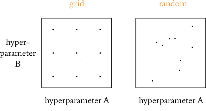
Figure 14.4 A strictly structured grid search (shown in the left-hand panel) is less likely to identify optimal hyperparameters for a given model than a search over values that are sampled randomly over the same hyperparameter ranges (right-hand panel).
13. Snoek, J., et al. (2012). Practical Bayesian optimization of machine learning algorithms. Advances in Neural Information Processing Systems, 25. Code available at github.com/JasperSnoek/spearmint.
14. Figure 1.10 provides a portrait of Bengio.
15. Bergstra, J., & Bengio, Y. (2012). Random search for hyper-parameter optimization. Journal of Machine Learning Research, 13, 281–305.
Deep Learning Libraries
Throughout this book, we have used Keras to construct and run our deep learning models. There are, however, countless other deep learning libraries, and more pop up every year. In this section, we review the other leading options you have.
Keras and TensorFlow
TensorFlow is perhaps the best-known deep learning library, its name derived from the concept of tensors (arrays of information, e.g., model inputs x or activations a) flowing through operations (e.g., those that define the mathematics of artificial neurons like our “most important equation” from back in Figure 6.7). The TensorFlow library was originally developed for internal use at Google, and the tech giant open-sourced the project in 2015. Figure 14.5 illustrates the relative interest in five of the most popular deep learning libraries, as per frequency of Google searches. Keras is the clear runner-up, with Tensor-Flow in the lead. Given this, you might be particularly interested in learning how to use TensorFlow. Well, we have good news for you: You already know how to.
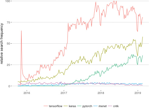
Figure 14.5 The relative Google search frequency (from October 2015 to February 2019) of five of the most popular deep learning libraries
Not only is Keras the high-level API that we’ve been using throughout this book to call TensorFlow in the background, but also—as of the release of TensorFlow 2.0 in 2019—Keras layers are the recommended approach for building models directly with the TensorFlow library itself. To build TensorFlow models in earlier versions of the software, it was necessary to become familiar with a fairly abstruse three-step process:
Configuring a detailed “computational graph”
Initializing this computational graph within a “session”
Feeding data into the session while fetching information you’d like to access (e.g., summary metrics, model parameters) out of the session
This relatively esoteric process was in place because it enabled TensorFlow to optimize the execution of deep learning model training and production-time execution across as many devices (CPUs and GPUs, perhaps spread across multiple servers) as are made available to it. In time, the developers behind libraries like PyTorch devised creative mechanisms to facilitate the best of both worlds:
The conceptually simple, layer-focused, instantly executable building of deep learning models and simultaneously . . .
The highly optimized model execution across however many devices are available
The team behind TensorFlow responded by more tightly incorporating Keras layers and by creating Eager mode—an approach to enable immediate execution (in place of the previous three-step process) without sacrificing performance. Prior to TensorFlow 2.0, Eager mode needed to be activated in order to use it,16 but from 2.0 onward it’s the built-in default.
16. With a single line of code: tf.enable_eager_execution().
Converting any of the code we covered in this book from being run with the Keras library to being run within TensorFlow itself is painless. For example, have a look at our Deep Net in TensorFlow notebook, which is identical to our Deep Net in Keras notebook (from Chapter 9) except for how the dependencies are loaded (Example 14.1, as compared to Examples 5.1 and 9.4).
Example 14.1 Dependencies for building a Keras layer-based deep net in TensorFlow without loading the Keras library
import tensorflow as tf
from tensorflow.python.keras.datasets import mnist
from tensorflow.python.keras.models import Sequential
from tensorflow.python.keras.layers import Dense, Dropout
from tensorflow.python.keras.layers import BatchNormalization
from tensorflow.python.keras.optimizers import SGD
from tensorflow.python.keras.utils import to_categorical
From there, you can begin exploring the added functionality and flexibility that Tensor-Flow offers.
Particular reasons you might use TensorFlow with Keras layers instead of the high-level Keras API alone include:
Customizing your model to your heart’s content, including by subclassing
tf.keras.Modelto forward propagate through your model in any way that you fancy17Creating high-performance data-input pipelines by using
tf.dataDeploying your model to
High-performance systems on servers with TensorFlow Serving
Mobile or embedded devices with TensorFlow Lite
A web browser with TensorFlow.js
PyTorch
PyTorch is the cousin of a machine learning framework called Torch, which is based in the programming language Lua. It’s really an extension of Torch, designed to feel fast and intuitive in the much more widely used Python language. PyTorch is developed primarily by the Facebook AI Research group led by Yann LeCun (Figure 1.9). Although not quite as popular as TensorFlow or Keras, PyTorch has gained a lot of traction in a short period of time (see Figure 14.5) and with good reason, as we elaborate on here.
Many high-level deep learning libraries (including Keras) serve as simple wrappers for low-level code (sometimes in Python, and sometimes in other languages such as C); however, PyTorch is not a simple Python wrapper for Torch. Rather, PyTorch was completely rewritten and specifically tailored to feel native to people familiar with Python, while retaining the computational efficiency of the original Torch library.
At its core, PyTorch performs matrix operations, much like NumPy. Indeed, PyTorch’s tensors are compatible with most NumPy operations, and methods exist for converting between NumPy arrays and PyTorch tensors. Because of this deep integration with NumPy, custom layers can be written directly in Python if this extra flexibility is desired. Unlike NumPy, however, PyTorch has specific systems in place to execute its calculations on GPUs, thereby leveraging these processors’ massively parallel matrix-calculation capabilities. Additionally, acceleration libraries are built in, which helps to make PyTorch fast regardless of device, and custom memory allocators enable it to be memory efficient.
If you’d like to learn more, in Appendix C we delve into many of the features of the PyTorch library. We compare and contrast it with TensorFlow, and we provide a hands-on demonstration of training a deep learning model. As you’ll see, the syntax of PyTorch is similar to that of Keras, and you should be able to pick it up fairly quickly if you so desire.
MXNet, CNTK, Caffe, and So On
Beyond Keras, TensorFlow, and PyTorch, there are myriad other deep learning libraries out there. Examples include:
MXNet, which was developed by Amazon.
CNTK, the Microsoft Cognitive Toolkit.
Caffe, out of the University of Berkeley, which is designed exclusively for machine vision/CNN applications. Caffe2, its lightweight successor, was being developed by Facebook AI Research, but it was folded into FAIR’s PyTorch project in 2018.
Theano, a University of Montreal project that once rivaled TensorFlow as the leading deep learning library, but is no longer in development largely because many of its developers jumped ship to Google’s TensorFlow project.
All of these libraries—indeed, any popular ones—are open-source. In addition, because the vast majority of these libraries follow the layer-focused design of Keras and have a similar syntax, you should have little trouble recognizing their code and employing them yourself if you have the inclination to.
Software 2.0
The models that all of the available deep learning libraries facilitate are revolutionizing the world of software. In a widely shared blog post written by the prominent data scientist Andrej Karpathy (Figure 14.6),18 he argues that deep learning is facilitating “Software 2.0.” Software 1.0 is what Karpathy describes as classic computer programming languages like Python, Java, JavaScript, C++, and so on. With Software 1.0, we need to provide explicit instructions within a computer program in order to have the computer produce outputs in the desired manner.

Figure 14.6 Andrej Karpathy is the director of AI at Tesla, the California-based automotive and energy firm. We mentioned him once earlier—in a footnote in Chapter 10. Karpathy’s background spans many institutions mentioned in this book, including OpenAI (Figure 4.13 and Chapter 13), Stanford University (where he completed his PhD under Fei-Fei Li; see Figure 1.14), DeepMind (e.g., Figures 4.4 through 4.10), Google (countless mentions across this book, including as the developers behind TensorFlow), and the University of Toronto (e.g., Figures 1.16 and Figure 3.2).
18. bit.ly/AKsoftware2
Software 2.0, in contrast, consists of deep learning models that approximate functions, like the functions we approximated in this book in order to classify handwritten digits, predict house prices, analyze the sentiment of film reviews, generate sketches of apples, and converge on Q* in order to play the Cart-Pole game. The millions or billions of parameters in productionized deep learning models today are increasingly demonstrating themselves to be more adaptable, useful, and powerful than hard-coded Software 1.0. Software 2.0 doesn’t replace Software 1.0, however: It builds on top of it, with Software 1.0 providing all of the critical digital infrastructure that Software 2.0 exists within.
Some of the particular advantages of Software 2.0 covered by Karpathy are:
Computational homogeneity: Deep learning models are made up of homogenous units—such as ReLU neurons—enabling matrix computations with these units to be highly optimizable and scalable.
Constant running time: Once making inferences in production systems, a given deep learning model will use the same amount of compute regardless of the input fed into it. Software 1.0 approaches, which could involve countless if-else statements, could require widely varying amounts of compute depending on the particular input fed into it.
Constant memory use: For the same reasons as the preceding point, a given deep learning model in production requires the same amount of memory resources regardless of the particular input fed into it.
Easy: By reading this one book, you’ve developed the skills to create high-performing algorithms across a range of domains. Prior to the advent of deep learning, markedly more domain-specific expertise would have been required to do this in each individual domain.
Superior: As we review in the next paragraph, deep learning models can dramatically outperform other approaches.
In light of these points, let’s review the applications that were featured in Part III of this book:
Machine vision (e.g., the MNIST digit recognition from Chapter 10): With traditional machine learning, this required hard-coding visual features extensively, typically requiring years of expertise in the field. Deep learning models perform better (recall Figure 1.15), learn features automatically, and require little vision-specific expertise to deploy effectively.
Natural language processing (e.g., the sentiment analysis from Chapter 11): In the traditional machine learning approach, many years of linguistics experience would typically be required to build an effective algorithm, including an understanding of the unique syntax and semantics of any given language involved in the application. Here too, deep learning models tend to perform better (as suggested by Figure 2.3). They learn the relevant features automatically, and again they require minimal linguistics-specific expertise to use effectively.
Simulating art and visual imagery (e.g., the drawings in Chapter 12): Generative adversarial networks, which incorporate deep learning models, produce far more compelling and realistic images than any preexisting approaches.19
Game-playing (e.g., the Deep Q-Learning networks in Chapter 13): A single algorithm, AlphaZero, can crush any Software 1.0 or traditional machine learning approach to playing Go, chess, and shogi (as shown in Figure 4.10). Remarkably, it does so more efficiently and doesn’t require any training data.
19. Visit distill.pub/2017/aia to experience an interactive article by Shan Carter and Michael Nielsen that expounds on how GANs can be used to augment human intelligence.
Approaching Artificial General Intelligence
Recalling the development of vision in trilobites from Chapter 1 (Figure 1.1), many millions of years passed before biological life evolved the sophisticated, full-color visual systems that primates like us benefit from. In contrast, it was a matter of decades from the first computer-vision systems (Figure 1.8) to ones that could match or exceed the performance of humans at visual-recognition tasks (Figure 1.15).20 Whereas image classification is a classic example of artificial narrow intelligence (ANI), rapid advancements such as this lead many researchers to believe that artificial general intelligence (AGI) and maybe even artificial super intelligence (ASI) can be attained in our lifetimes.21 The Müller and Bostrom survey results we mentioned back in Chapter 1, for example, have median estimates of 2040 and 2060 for the genesis of AGI and ASI, respectively.
20. The human-accuracy benchmark in Figure 1.15 is Andrej Karpathy (Figure 14.6) himself, by the way.
21. Refer back to the end of Chapter 1 for a refresher on ANI, AGI, and ASI.
Four primary factors are driving our rapid advances in ANI and also may be hurrying us in the direction of AGI or ASI:
Data: In recent years, the amount of data in the digital realm doubles about every 18 months. This exponential rate of growth shows no sign of slowing (recall from Chapter 13, for example, the relentless swell of data produced by an individual autonomous vehicle). A lot of the data is low quality, but—as with the open data sources we mentioned earlier in this chapter—datasets are becoming larger, cheaper to store, and often better organized (ImageNet from Chapters 1 and 10 is an exemplar).
Computing power: Although the rate of performance improvements on individual CPUs may slow down in coming years,22 the massive parallelization of matrix operations within GPUs and across many servers—each with multiple CPUs and perhaps multiple GPUs—will continue to increase the ready availability of compute.
Algorithms: A rapidly enlarging army of data-focused scientists and engineers—who are global, and who are spread across both the academic and commercial realms—is tweaking the techniques used to mine datasets for meaningful patterns. Every once in a while, there is a breakthrough like AlexNet (Figure 1.15). In recent years, deep learning has been associated with the bulk of these breakthroughs, many of which we’ve covered over the course of this book.
Infrastructure: The Software 1.0 infrastructure such as open-source operating systems and programming languages, paired with Software 2.0 libraries and techniques (shared in nearly real time, worldwide, via arXiv and GitHub) and the low cost of cloud-computing providers (e.g., Amazon Web Services, Microsoft Azure, Google Cloud Platform) provide a highly scalable hotbed for approaches to be experimented with on ever-larger datasets.
22. Moore’s “law” is anything but a law, and the shrinking of transistors down toward electron scale makes decreasing the cost of computation on a given chip trickier and trickier.
The cognitive tasks that humans tend to find hard (e.g., playing chess, solving matrix algebra problems, optimizing a financial portfolio) are generally the ones that Homo sapiens have been doing for only thousands of years or fewer; these are the types of tasks that today tend to be easy for machines. In contrast, the cognitive tasks humans find easy (e.g., reading social cues, carrying an infant safely up the stairs) evolved over millions of years and today remain beyond the reach of machines. So despite all of the justifiable excitement around machine learning, the possibility of AGI could be a long way off and remains only a theoretical possibility at this time. Some examples of the significant barriers that prevent contemporary deep learning from bringing about AGI include:23
23. For more on the limitations of deep learning, read Marcus, G. (2018). Deep learning: A critical appraisal. arXiv: 1801.00631.
Deep learning requires training on many, many samples. These large datasets are not always available, and, in stark contrast, biological learning systems—including those in mice and human infants—can often learn from a single example.
Deep learning models are typically a black box. Although investigative techniques like Jason Yosinski and colleagues’ DeepViz tool24 exist, these are the exceptions to the rule.
Deep learning models don’t leverage knowledge of the world; they don’t, for example, take into account databases of facts when they make inferences.
To deep learning models, a predicted correlation between some input x and some outcome y provides no assessment of causation. Being able to move beyond predicting correlations between variables toward causal relationships between them is presumably critical to the development of general intelligence.
Deep learning models are often susceptible to unintuitive and embarrassing failures,25 and they can be deliberately duped by changes to even a single pixel in an input image.26
24. bit.ly/DeepViz
25. Go to bit.ly/googleGaffe for an infamous example.
26. Deliberately misleading a machine learning algorithm is called an adversarial attack, and it is carried out by inputting an adversarial example. There are many papers on these; one outlining single-pixel adversarial attacks on CNNs is Su, J., et al. (2017). One pixel attack for fooling deep neural networks. arXiv: 1710.08864.
Perhaps some of these barriers catch your own interest, and you could consider dedicating some of your career to contributing to devising solutions! We can’t know precisely what the future will hold, but given the explosions of data, compute, algorithms, and infrastructure, one prediction we’re confident making is that you should have little difficulty identifying exhilerating opportunities to apply deep learning.
Summary
This chapter wrapped up the book by providing you with project ideas, resources for further learning, a general guide to fitting models, an overview of the deep learning models available to you beyond Keras, and an exploration of the ways artificial neural networks are rapidly reshaping software—with much more potential excitement in the years to come!
Have fun going forward, and please do stay in touch:
Here’s a Twitter account we use for posting about new content as it’s released, including new studio-recorded video tutorials we anticipate publishing to accompany the material covered in this book: twitter.com/JonKrohnLearns
We use Medium for long-form blog posts: medium.com/@jonkrohn
We set up a Google Group to enable readers of this book to ask questions and have them answered by other readers (perhaps even us!) in a forum format. You can find it here:
bit.ly/DLIforumAnd, finally, feel free to add us on LinkedIn (e.g., linkedin.com/in/jonkrohn), but be sure to mention you’re a reader because we don’t accept requests from just anyone!
We hope you enjoyed this visual, interactive introduction to deep learning. We’re deeply grateful for the time and energy you invested in this journey that you’ve taken alongside us. Farewell, dear friend—from the amiable trilobite in Figure 14.7.

Figure 14.7 Trilobyte waving good-bye