Chapter 16
Advanced calculations in DAX
In this last chapter about the features of the DAX language and before discussing optimization, we want to show several examples of calculations performed with DAX. The goal of this chapter is not to provide ready-to-use patterns that one can use out of the box; these patterns are available at https://www.daxpatterns.com. Instead, the goal is to show formulas of different levels of complexity to exercise your mind in the fascinating art of “thinking in DAX.”
DAX does indeed require your brain to think creatively. Now that you have learned all the secrets of the language, it is time to put everything into practice. From the next chapter onwards, we will start to cover optimization. Therefore, in this chapter we start bringing up measure performance, providing the first clues as to how to measure the complexity of a formula.
Here, the goal is not to try to achieve the best performance because performance analysis requires knowledge that you will only learn in later chapters. Nevertheless, in this chapter we provide different formulations of the same measure, analyzing the complexity of each version. Being able to author several different versions of the same measure is a skill that will be of paramount importance in performance optimization.
Computing the working days between two dates
Given two dates, one can compute the difference in days by using a simple subtraction. In the Sales table there are two dates: the delivery date and the order date. The average number of days required for delivery can be obtained with the following measure:
Avg Delivery :=
AVERAGEX (
    Sales,
    INT ( Sales[Delivery Date] - Sales[Order Date] + 1)
)
Because of the internal format of a DateTime, this measure produces an accurate result. Yet it would be unfair to consider that an order received on Friday and shipped on Monday took three days to deliver, if Saturdays and Sundays are considered nonworking days. In fact, it only took one working day to ship the order—same as if the order had been received on Monday and shipped on Tuesday. Therefore, a more accurate calculation should consider the difference between the two dates expressed in working days. We provide several versions of the same calculation, seeking for the best in terms of performance and flexibility.
Excel provides a specific function to perform that calculation: NETWORKDAYS. However, DAX does not offer an equivalent feature. DAX offers the building blocks to author a complex expression that computes the equivalent of NETWORKDAYS, and much more. For example, a first way to compute the number of working days between two dates is to count the number of days between the two dates that are working days:
Avg Delivery WD :=
AVERAGEX (
Sales,
VAR RangeOfDates =
DATESBETWEEN (
'Date'[Date],
Sales[Order Date],
Sales[Delivery Date]
)
VAR WorkingDates =
FILTER (
RangeOfDates,
NOT ( WEEKDAY ( 'Date'[Date] ) IN { 1, 7 } )
)
VAR NumberOfWorkingDays =
COUNTROWS ( WorkingDates )
RETURN
NumberOfWorkingDays
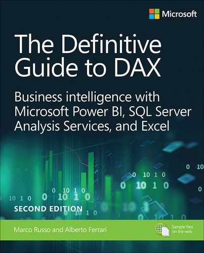
)For each row in Sales, the measure creates a temporary table in RangeOfDates with all the dates in between the order and delivery dates. Then, it filters out Saturdays and Sundays in WorkingDates, and finally it counts the number of rows that survived the filter in NumberOfWorkingDays. Figure 16-1 shows a line chart with the difference between the average delivery time in days and in working days.
The measure works well, with a few shortcomings. First, it does not consider holidays. For example, by removing Saturdays and Sundays, the first of January is considered a regular working day, provided it does not fall on a weekend. The same happens for any other holidays in the year. Second, the performance of the formula can be improved.
In order to handle holidays, one needs to store the information about whether a given day is a holiday or not in a table. The Date table is the perfect place for this, in a column named Is Holiday. Then, the formula should use other columns of the Date table instead of just using the Date[Date] column like the previous measure did:
Avg Delivery WD DT :=
AVERAGEX (
    Sales,
    VAR RangeOfDates =
        DATESBETWEEN (
            'Date'[Date],
            Sales[Order Date],
            Sales[Delivery Date]
        )
    VAR NumberOfWorkingDays =
        CALCULATE (
            COUNTROWS ( 'Date' ),
            RangeOfDates,
            NOT ( WEEKDAY ( 'Date'[Date] ) IN { 1, 7 } ),
            'Date'[Is Holiday] = 0
        )
    RETURN
        NumberOfWorkingDays
)
Now that the measure is more data-driven, one could also store the information about the weekend in the Date table, replacing the test with WEEKDAY with a new column containing Workday or Weekend. This reduces the complexity of the measure and moves most of the logic into the data, gaining in flexibility.
In terms of complexity, the measure performs two operations:
An iteration over the Sales table.
For each row in Sales, the creation of a temporary table with all the dates between the order and delivery dates.
If there are one million rows in Sales and the average for delivery days is seven, the complexity of the measure is around seven million. Indeed, the engine needs to build a temporary table with around seven rows, one million times.
It is possible to reduce the complexity of the formula by reducing either the number of iterations performed by AVERAGEX or the number of rows in the temporary table with the business days. An interesting point is that the calculation is not necessary at the individual sale level. Indeed, all the orders with the same Order Date and Delivery Date share the same duration. Thus, it is possible to first group all the orders by Order Date and Delivery Date, then compute the duration of these pairs of dates for a reduced number of rows. By doing so, we can reduce the number of iterations performed by AVERAGEX, but at the same time we lose information about how many orders each pair of dates was pertaining to. This can be resolved by transforming the simple average into a weighted average, using the number of orders as the weight for the average.
This idea is implemented in the following code:
Avg Delivery WD WA :=
VAR NumOfAllOrders =
    COUNTROWS ( Sales )
VAR CombinationsOrderDeliveryDates =
    SUMMARIZE (
        Sales,
        Sales[Order Date],
        Sales[Delivery Date]
    )
VAR DeliveryWeightedByNumOfOrders =
    SUMX (
        CombinationsOrderDeliveryDates,
        VAR RangeOfDates =
            DATESBETWEEN (
                'Date'[Date],
                Sales[Order Date],
                Sales[Delivery Date]
            )
        VAR NumOfOrders =
            CALCULATE (
                COUNTROWS ( Sales )
            )
        VAR WorkingDays =
            CALCULATE (
                COUNTROWS ( 'Date' ),
                RangeOfDates,
                NOT ( WEEKDAY ( 'Date'[Date] ) IN { 1, 7 } ),
                'Date'[Is Holiday] = 0
            )
        VAR NumberOfWorkingDays = NumOfOrders * WorkingDays
        RETURN
            NumberOfWorkingDays
    )
VAR AverageWorkingDays =
    DIVIDE (
        DeliveryWeightedByNumOfOrders,
        NumOfAllOrders
    )
RETURN
    AverageWorkingDays
The code is now much harder to read. An important question is: is it worth making the code more complex just to improve performance? As always, it depends. Before diving into this kind of optimization, it is always useful to perform some tests to check if the number of iterations is indeed reduced. In this case, one could evaluate the benefits by running the following query, which returns the total number of rows and the number of unique combinations of Order Date and Delivery Date:
EVALUATE
{ (
    COUNTROWS ( Sales ),
    COUNTROWS (
        SUMMARIZE (
            Sales,
            Sales[Order Date],
            Sales[Delivery Date]
        )
    )
) }

-- The result is:
--
-- Value1  |  Value2
--------------------
-- 100231  |    6073
In the demo database there are 100,231 rows in Sales and only 6,073 distinct combinations of order and delivery dates. The more complex code in the Avg Delivery WD WA measure reduces the number of iterations by a bit more than an order of magnitude. Therefore, in this case authoring more complex code is worth the effort. You will learn how to evaluate the impact on execution time in later chapters. For now, we focus on code complexity.
The complexity of the Avg Delivery WD WA measure depends on the number of combinations of order and delivery dates, and on the average duration of an order. If the average duration of an order is just a few days, then the formula runs very fast. If the average duration of an order is of several years, then performance might start to be an issue because the result of DATESBETWEEN starts to be a large table with hundreds of rows.
Because the number of nonworking days is usually smaller than the number of working days, an idea could be to count nonworking days instead of counting working days. Therefore, another algorithm might be the following:
Compute the difference between the two dates in days.
Compute the number of nonworking days in between the two dates.
Subtract the values computed in (1) and (2).
One can implement this with the following measure:
Avg Delivery WD NWD :=
VAR NonWorkingDays =
    CALCULATETABLE (
        VALUES ( 'Date'[Date] ),
        WEEKDAY ( 'Date'[Date] ) IN { 1, 7 },
        ALL ( 'Date' )
    )
VAR NumOfAllOrders =
    COUNTROWS ( Sales )
VAR CombinationsOrderDeliveryDates =
    SUMMARIZE (
        Sales,
        Sales[Order Date],
        Sales[Delivery Date]
    )
VAR DeliveryWeightedByNumOfOrders =
    CALCULATE (
        SUMX (
            CombinationsOrderDeliveryDates,
            VAR NumOfOrders =
                CALCULATE (
                    COUNTROWS ( Sales )
                )
            VAR NonWorkingDaysInPeriod =
                FILTER (
                    NonWorkingDays,
                    AND (
                        'Date'[Date] >= Sales[Order Date],
                        'Date'[Date] <= Sales[Delivery Date]
                    )
                )
            VAR NumberOfNonWorkingDays =
                COUNTROWS ( NonWorkingDaysInPeriod )
            VAR DeliveryWorkingDays =
                Sales[Delivery Date] - Sales[Order Date] - NumberOfNonWorkingDays + 1
            VAR NumberOfWorkingDays =
                NumOfOrders * DeliveryWorkingDays
            RETURN
                NumberOfWorkingDays
        )
    )
VAR AverageWorkingDays =
    DIVIDE (
        DeliveryWeightedByNumOfOrders,
        NumOfAllOrders
    )
RETURN
    AverageWorkingDays
This code runs more slowly than the previous code in the database used for this book. Regardless, this version of the same calculation might perform better on a different database where orders have a much larger duration. Only testing will point you in the right direction.
Finally, be mindful that when seeking optimal performance, nothing beats precomputing the values. Indeed, no matter what, the difference in working days between two dates always leads to the same result. We already know that there are around 6,000 combinations of order and delivery dates in our demo data model. One could precompute the difference in working days between these 6,000 pairs of dates and store the result in a physical, hidden table. Therefore, at query time there is no need to compute the value. A simple lookup of the result provides the number needed.
Therefore, an option is to create a physical hidden table with the following code:
WD Delta =
ADDCOLUMNS (
    SUMMARIZE (
        Sales,
        Sales[Order Date],
        Sales[Delivery Date]
    ),
    "Duration", [Avg Delivery WD WA]
)
Once the table is in the model, we take advantage of the precomputed differences in working days by modifying the previous best formula with the following:
Avg Delivery WD WA Precomp :=
VAR NumOfAllOrders =
    COUNTROWS ( Sales )
VAR CombinationsOrderDeliveryDates =
    SUMMARIZE (
        Sales,
        Sales[Order Date],
        Sales[Delivery Date]
    )
VAR DeliveryWeightedByNumOfOrders =
    SUMX (
        CombinationsOrderDeliveryDates,
        VAR NumOfOrders =
            CALCULATE (
                COUNTROWS ( Sales )
            )
        VAR WorkingDays =
            LOOKUPVALUE (
                'WD Delta'[Duration],
                'WD Delta'[Order Date], Sales[Order Date],
                'WD Delta'[Delivery Date], Sales[Delivery Date]
            )
        VAR NumberOfWorkingDays = NumOfOrders * WorkingDays
        RETURN
            NumberOfWorkingDays
    )
VAR AverageWorkingDays =
    DIVIDE (
        DeliveryWeightedByNumOfOrders,
        NumOfAllOrders
    )
RETURN
    AverageWorkingDays
It is very unlikely that this level of optimization would be required for a simple calculation involving the number of working days between two dates. That said, we were not trying to demonstrate how to super-optimize a measure. Instead, we wanted to show several different ways of obtaining the same result, from the most intuitive version down to a very technical and optimized version that is unlikely to be useful in most scenarios.
Showing budget and sales together
Consider a data model that contains budget information for the current year, along with actual sales. At the beginning of the year, the only available information is the budget figures. As time goes by, there are actual sales, and it becomes interesting both to compare sales and budget, and to adjust the forecast until the end of the year by mixing budget and actual sales.
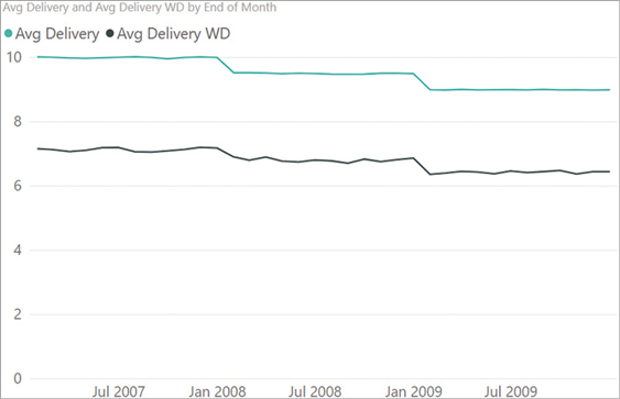
To simulate this scenario, we removed all the sales after August 15, 2009, and we created a Budget table containing the daily budget for the entire year 2009. The resulting data is visible in Figure 16-2.
The business question is: provided that on August 15, the Sales Amount is 24 million, what should be the adjusted forecast at the end of the year, using actuals for the past and budget for the future? Be mindful that because sales ended on the 15th, in August there should be a mix of sales and budget.
The first step is determining the date where sales stop. Using a simple function like TODAY would be misleading because data in the model are not necessarily updated to the current day. A better approach is to search for the last date with any data in the Sales table. A simple MAX works well, but it is important to note that user selection might have a negative effect on the result. For example, consider the following measure:
LastDateWithSales := MAX ( 'Sales'[OrderDateKey] )
Different brands, or in general different selections, might return different dates. This is shown in Figure 16-3.

An appropriate way to compute the last date with any sales is to remove all the filters before computing the maximum date. This way, August 15, 2009, is used for all the products. If any brand does not have any sales on August 15, the value to use is zero, not the budget of the last day with sales for that brand. Therefore, the correct formulation for LastDateWithSales is the following:
LastDateWithSales :=
CALCULATE (
    MAX ( 'Sales'[OrderDateKey] ),
    ALL ( Sales )
)
By removing the filter from Sales (which is the expanded Sales table), the code is ignoring any filter coming from the query, always returning August 15, 2009. At this point, one needs to write code that uses the value of Sales Amount for all the dates before the last date with any sales, and the value of Budget Amt for the dates after. One simple implementation is the following:
Adjusted Budget :=
VAR LastDateWithSales =
    CALCULATE (
        MAX ( Sales[OrderDateKey] ),
        ALL ( Sales )
    )
VAR AdjustedBudget =
    SUMX (
        'Date',
        IF (
            'Date'[DateKey] <= LastDateWithSales,
            [Sales Amount],
            [Budget Amt]
        )
    )
RETURN AdjustedBudget
Figure 16-4 shows the result of the new Adjusted Budget measure.

At this point, we can investigate the measure’s complexity. The outer iteration performed by SUMX iterates over the Date table. In a year, it iterates 365 times. At every iteration, depending on the value of the date, it scans either the Sales or the Budget table, performing a context transition. It would be good to reduce the number of iterations, thus reducing the number of context transitions and/or aggregations of the larger Sales and Budget tables.
Indeed, a good solution does not need to iterate over the dates. The only reason to perform the iteration is that the code is more intuitive to read. A slightly different algorithm is the following:
Split the current selection on Date in two sets: before and after the last date with sales.
Compute the sales for the previous period.
Compute the budget for the future.
Sum sales and budget computed earlier during (2) and (3).
Moreover, there is no need to compute sales just for the period before the last date. Indeed, there will be no sales in the future, so there is no need to filter dates when computing the amount of sales. The only measure that needs to be restricted is the budget. In other words, the formula can sum the entire amount of sales plus the budget of the dates after the last date with sales. This leads to a different formulation of the Adjusted Budget measure:
Adjusted Budget Optimized :=
VAR LastDateWithSales =
    CALCULATE (
        MAX ( Sales[OrderDateKey] ),
        ALL ( Sales )
    )
VAR SalesAmount = [Sales Amount]
VAR BudgetAmount =
    CALCULATE (
        [Budget Amt],
        KEEPFILTERS ( 'Date'[DateKey] > LastDateWithSales )
    )
VAR AdjustedBudget = SalesAmount + BudgetAmount
RETURN
    AdjustedBudget
The results from Adjusted Budget Optimized are identical to those of the Adjusted Budget measure, but the code complexity is much lower. Indeed, the code of Adjusted Budget Optimized only requires one scan of the Sales table and one scan of the Budget table, the latter with an additional filter on the Date table. Please note that KEEPFILTERS is required. Otherwise, the condition on the Date table would override the current context, providing incorrect figures. This final version of the code is slightly harder to read and to understand, but it is much better performance-wise.
As with previous examples, there are different ways of expressing the same algorithm. Finding the best way requires experience and a solid understanding of the internals of the engine. With that said, simple considerations about the cardinality required in a DAX expression already help a lot in optimizing the code.
Computing same-store sales
This scenario is one specific case of a much broader family of calculations. Contoso has several stores all around the world, and each store has different departments, each one selling specific product categories. Departments are continuously updated: Some are opened, others are closed or renewed. When analyzing sales performance, it is important to compare like-for-like—that is, analyze the sales behavior of comparable departments. Otherwise, one might erroneously conclude that a department performed very poorly, just because for some time in the selected period it had been closed down.
The like-for-like concept can be tailored to every business. In this example, the requirement is to exclusively compare stores and product categories that have sales in the years considered for the analysis. For each product category, a report should solely include stores that have sales in the same years. Variations to this requirement might use the month or the week as granularity in the like-for-like comparison, without changing the approach described as follows.
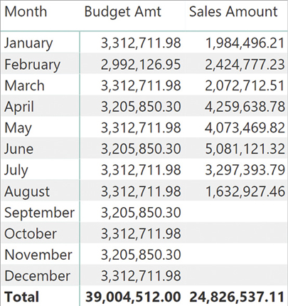
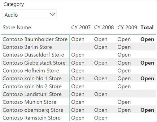
For example, consider the report in Figure 16-5, which analyzes the sales of one product category (Audio) in German stores over three calendar years.
The Berlin store was closed in 2007. Out of the two stores in Koln, one was under maintenance in 2008; it was thus only open two out of the three years considered. In order to achieve a fair comparison of the values calculated, any analysis of sales trends needs to be restricted to stores within the selection that were always open.
Because the rules of a like-for-like comparison can be complex and require different types of adjustments, it is a good idea to store the status of the comparable elements in a separate table. This way, any complexity in the business logic will not affect the query performance but only the time required to refresh the status table. In this example, the StoresStatus table contains one row for each combination of year, category, and store, alongside with status, which can be Open or Closed. Figure 16-6 shows the status of the German stores, only showing the Open status and hiding the Closed status to improve readability.
The most interesting column is the last one: Just four stores have been open for all three years. A relevant trend analysis should consider these four stores exclusively, for Audio sales. Moreover, if one changes the selection on the years, the status changes too. Indeed, if one only selects two years (2007 and 2008), the status of the stores is different, as shown in Figure 16-7.

The like-for-like measure must perform the following steps:
Determine the stores open in all the years of the report for each product category.
Use the result of the first step to filter the Amount measure, restricting the values to stores and product categories that have sales in all the years included in the report.
Before moving further with the example, a deeper analysis of the data model is required. The diagram view is represented in Figure 16-8.
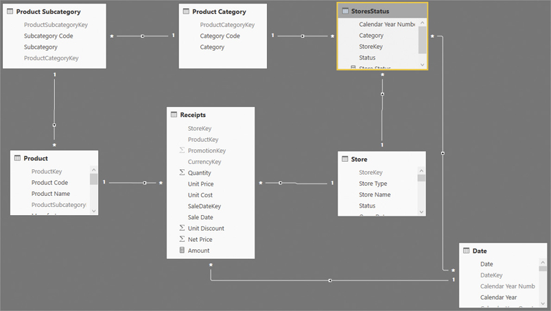
Let us point out a few things about the model:
The relationship between Date and StoreStatus is an MMR weak relationship based on Year, with the cross-filter direction going towards StoreStatus. Date filters StoreStatus, not the other way around.
The relationship between Product Category and StoreStatus is a regular one-to-many relationship.
All other relationships are regular one-to-many relationships, with a single cross-filter used in many other demos of this book.
StoreStatus contains one row for each store, product category, and year combination. The status of each row is either Open or Closed. In other words, there are no gaps in the table. This is relevant to reduce the complexity of the formula.
The first step is determining which departments are open over all the years selected. To obtain this, the code must filter the StoresStatus table with a given product category and all the selected years. If after having performed this filter, all the filtered rows contain Open in the status, then the department has been open over the whole time period. Otherwise, if there are multiple values (some Open, some Closed), this means that the department was closed at some point. The following query performs this calculation:
EVALUATE
VAR StatusGranularity =
    SUMMARIZE (
        Receipts,
        Store[Store Name],
        'Product Category'[Category]
    )
VAR Result =
    FILTER (
        StatusGranularity,
        CALCULATE (
            SELECTEDVALUE ( StoresStatus[Status] ),
            ALLSELECTED ( 'Date'[Calendar Year] )
        ) = "Open"
    )
RETURN
    Result
The query iterates at the store/category cardinality, and for each of these pairs it checks if the value of the Status is Open for all selected years. In case there are multiple values for StoreStatus[Status], the result of SELECTEDVALUE is blank preventing the pair from surviving the filter.
Once we can determine the set of departments open all of the years, the set obtained can be used as a filter to CALCULATE to obtain the result:
OpenStoresAmt :=
VAR StatusGranularity =
    SUMMARIZE (
        Receipts,
        Store[Store Name],
        'Product Category'[Category]
    )
VAR OpenStores =
    FILTER (
        StatusGranularity,
        CALCULATE (
            SELECTEDVALUE ( StoresStatus[Status] ),
            ALLSELECTED ( 'Date'[Calendar Year] )
        ) = "Open"
    )
VAR AmountLikeForLike =
    CALCULATE (
        [Amount],
        OpenStores
    )
RETURN
    AmountLikeForLike
Once projected in a matrix, the measure produces the report in Figure 16-9.

Stores that are not open all the time have disappeared from the report. It is important to learn this technique well because it is one of the most powerful and useful techniques in DAX. The ability to compute a table containing a filter and then use it to restrict the calculation is the foundation of several advanced calculations in DAX.
In this example, we used an additional table to store the information about whether a store is open or closed. We could have achieved a similar goal by inspecting the Receipts table alone, inferring whether a store was open or closed based on their sales. If there are sales, then the assumption is that the store was open. Unfortunately, the opposite is not quite true. The absence of sales does not imply that the store department selling that category was closed. In an unfortunate and borderline scenario, the absence of sales might simply mean that although the department was open, no sale took place.
This last consideration is more about data modeling than DAX, yet we felt it was important to mention it. In case one needs to retrieve the information about the store being open from the Receipts table, the formula requires more attention.
The following measure implements the OpenStoresAmt measure without using the StoresStatus table. For each pair of store and product category, the measure must check whether the number of years in which there are sales is the same as the number of years selected. If a store has sales for just two out of three years, this means that the considered department was closed for one year. The following code is a possible implementation:
OpenStoresAmt Dynamic :=
VAR SelectedYears =
    CALCULATE (
        DISTINCTCOUNT ( 'Date'[Calendar Year] ),
        CROSSFILTER ( Receipts[SaleDateKey], 'Date'[DateKey], BOTH ),
        ALLSELECTED ()
    )
VAR StatusGranularity =
    SUMMARIZE (
        Receipts,
        Store[Store Name],
        'Product Category'[Category]
    )
VAR OpenStores =
    FILTER (
        StatusGranularity,
        VAR YearsWithSales =
            CALCULATE (
                DISTINCTCOUNT ( 'Date'[Calendar Year] ),
                CROSSFILTER ( Receipts[SaleDateKey], 'Date'[DateKey], BOTH ),
                ALLSELECTED ( 'Date'[Calendar Year] )
            )
        RETURN
            YearsWithSales = SelectedYears
    )
VAR AmountLikeForLike =
    CALCULATE (
        [Amount],
        OpenStores
    )
RETURN
    AmountLikeForLike
The complexity of this latter version is much higher. Indeed, it requires moving the filter from the Receipts table to the Date table for every product category to compute the number of years with sales. Because—typically—the Receipts table is much larger than a table with only the status for the store, this code is slower than the previous solution based on the StoresStatus table. Nevertheless, it is useful to note that the only difference between the previous version and this one is in the condition inside FILTER. Instead of inspecting a dedicated table, the formula needs to scan the Receipts table. The pattern is still the same.
Another important detail of this code is the way it computes the SelectedYears variable. Here, a simple DISTINCTCOUNT of all the selected years would not fit. Indeed, the value to compute is not the number of all the selected years, but solely the selected years with sales. If there are 10 years in the Date table and just three of them have sales, using a simpler DISTINCTCOUNT would also consider the years with no sales, returning blank on every cell.
Numbering sequences of events
This section analyzes a surprisingly common pattern: the requirement to number sequences of events, to easily find the first, the last, and the previous event. In this example, the requirement is to number each order by customer in the Contoso database. The goal is to obtain a new calculated column that contains 1 for the first order of a customer, 2 for the second, and so on. Different customers will have the same number 1 for their first order.
![]() Warning
Warning
We should start with a big warning: Some of these formulas are slow. We show samples of code to discuss their complexity while searching for a better solution. If you plan to try them on your model, be prepared for a very long calculation time. By “long,” we mean hours of computation and tens of gigabytes of RAM used by the demo model provided. Otherwise, simply follow the description; we show a much better code at the end of the section.
The result to obtain is depicted in Figure 16-10.

A first way to compute the order position is the following: for one same customer, the code could count the number of orders that date prior to the current order. Unfortunately, using the date does not work because there are customers who placed multiple orders on the same day; this would generate an incorrect numbering sequence. Luckily, the order number is unique and its value increases for every order. Thus, the formula computes the correct value by counting for one same customer, the number of orders with an order number less than or equal to the current order number.
The following code implements this logic:
Sales[Order Position] =
VAR CurrentOrderNumber = Sales[Order Number]
VAR Position =
    CALCULATE (
        DISTINCTCOUNT ( Sales[Order Number] ),
        Sales[Order Number] <= CurrentOrderNumber,
        ALLEXCEPT (
            Sales,
            Sales[CustomerKey]
        )
    )
RETURN
    Position
Although it looks rather straightforward, this code is extremely complex. Indeed, in CALCULATE it uses a filter on the order number and the context transition generated by the calculated column. For each row in Sales, the engine must filter the Sales table itself. Therefore, its complexity is the size of Sales squared. Because Sales contains 100,000 rows, the total complexity is 100,000 multiplied by 100,000; that results in 10 billion. The net result is that this calculated column takes hours to compute. On a larger dataset, it would put any server on its knees.
We discussed the topic of using CALCULATE and context transition on large tables in Chapter 5, “Understanding CALCULATE and CALCULATETABLE.” A good developer should try to avoid using context transition on large tables; otherwise, they run the risk of incurring poor performance.
A better implementation of the same idea is the following: Instead of using CALCULATE to apply a filter with the expensive context transition, the code could create a table containing all the combinations of CustomerKey and Order Number. Then, it could apply a similar logic to that table by counting the number of order numbers lower than the current one for that same customer. Here is the code:
Sales[Order Position] =
VAR CurrentCustomerKey = Sales[CustomerKey]
VAR CurrentOrderNumber = Sales[Order Number]
VAR CustomersOrders =
    ALL (
        Sales[CustomerKey],
        Sales[Order Number]
    )
VAR PreviousOrdersCurrentCustomer =
    FILTER (
        CustomersOrders,
        AND (
            Sales[CustomerKey] = CurrentCustomerKey,
            Sales[Order Number] <= CurrentOrderNumber
        )
    )
VAR Position =
    COUNTROWS ( PreviousOrdersCurrentCustomer )
RETURN
    Position
This new formulation is much quicker. First, the number of distinct combinations of CustomerKey and Order Number is 26,000 instead of 100,000. Moreover, by avoiding context transition the optimizer can generate a much better execution plan.
The complexity of this formula is still high, and the code is somewhat hard to follow. A much better implementation of the same logic uses the RANKX function. RANKX is useful to rank a value against a table, and doing that it can easily compute a sequence number. Indeed, the sequence number of an order is the same value as the ascending ranking of the order in the list of all the orders of the same customer.
The following is an implementation of the same calculation as the previous formula, this time using RANKX:
Sales[Order Position] =
VAR CurrentCustomerKey = Sales[CustomerKey]
VAR CustomersOrders =
    ALL (
        Sales[CustomerKey],
        Sales[Order Number]
    )
VAR OrdersCurrentCustomer =
    FILTER (
        CustomersOrders,
        Sales[CustomerKey] = CurrentCustomerKey
    )
VAR Position =
    RANKX (
        OrdersCurrentCustomer,
        Sales[Order Number],
        Sales[Order Number],
        ASC,
        DENSE
    )
RETURN
    Position
RANKX is very well optimized. It has an efficient internal sorting algorithm that lets it execute quickly even on large datasets. On the demo database the difference between the last two formulas is not very high, yet a deeper analysis of the query plan reveals that the version with RANKX is the most efficient. The analysis of query plans is a topic discussed in the next chapters of the book.
Also, in this example there are multiple ways of expressing the same code. Using RANKX to compute a sequence number might not be obvious to a DAX novice, which is the reason we included this example in the book. Showing different versions of the same code provides food for thought.
Computing previous year sales up to last date of sales
The following example extends time intelligence calculations with more business logic. The goal is to compute a year-over-year comparison accurately, ignoring in the previous year any sales that took place after a set date. To demonstrate the scenario, we removed from the demo database all sales after August 15, 2009. Therefore, the last year (2009) is incomplete, and so is the month of August 2009.
Figure 16-11 shows that sales after August 2009 report empty values.

When the month is present on the report as in the report shown, the numbers are clear. A user would quickly understand that the last year is incomplete; therefore, they would not make a comparison between the total of 2009 against the total of previous years. Nevertheless, a developer could author some code that—despite being useful—makes the wrong decisions. Consider the following two measures:
PY Sales :=
CALCULATE (
    [Sales Amount],
    SAMEPERIODLASTYEAR ( 'Date'[Date] )
)

Growth :=
DIVIDE (
    [Sales Amount] - [PY Sales],
    [PY Sales]
)
A user might easily build a report like the one in Figure 16-12 and erroneously deduce that sales are decreasing dramatically for all the brands.
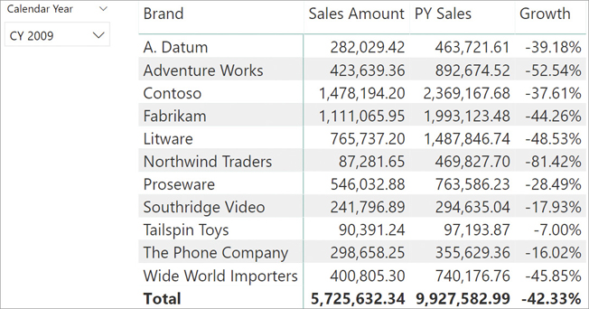
The report does not perform a fair comparison between 2008 and 2009. For the selected year (2009), it reports the sales up to August 15, 2009, whereas for the previous year it considers the sales of the entire year, including September and later dates.
An appropriate comparison should exclusively consider sales that occurred before August 15 in all previous years, so to produce meaningful growth percentages. In other words, the data from previous years should be restricted to the dates up to the last day and month of sales in 2009. The cutoff date is the last date for which there are sales reported in the database.
As usual, there are several ways to solve the problem, and this section presents some of them. The first approach is to modify the PY Sales measure, so that it only considers the dates that happen to be before the last date of sales projected in the previous year. One option to author the code is the following:
PY Sales :=
VAR LastDateInSales =
CALCULATETABLE (
LASTDATE ( Sales[Order Date] ),
ALL ( Sales )
)
VAR LastDateInDate =
TREATAS (
LastDateInSales,
'Date'[Date]
)
VAR PreviousYearLastDate =
SAMEPERIODLASTYEAR ( LastDateInDate )
VAR PreviousYearSales =
CALCULATE (
[Sales Amount],
SAMEPERIODLASTYEAR ( 'Date'[Date] ),
'Date'[Date] <= PreviousYearLastDate
)
RETURN
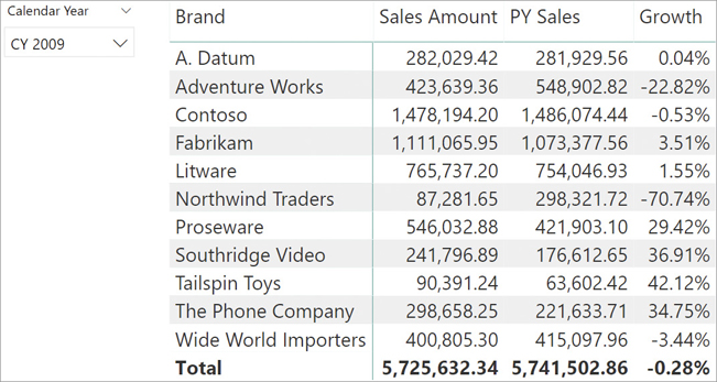
PreviousYearSalesThe first variable computes the last Order Date in all sales. In the sample data model, it retrieves August 15, 2009. The second variable (LastDateInDate) changes the data lineage of the previous result to Date[Date]. This step is needed because time intelligence functions are expected to work on the date table. Using them on different tables might lead to wrong behaviors, as we will demonstrate later. Once LastDateInDate contains August 15, 2009, with the right data lineage, SAMEPERIODLASTYEAR moves this date one year back. Finally, CALCULATE uses this value to compute the sales in the previous year combining two filters: the current selection moved one year back and every day before August 15, 2008.
The result of this new formula is visible in Figure 16-13.
It is important to understand the reason why the previous formula requires TREATAS. An inexperienced DAX developer might write the same measure with this simpler code:
PY Sales Wrong :=
VAR LastDateInSales =
    CALCULATETABLE (
        LASTDATE ( Sales[Order Date] ),
        ALL ( Sales )
    )
VAR PreviousYearLastDate =
    SAMEPERIODLASTYEAR ( LastDateInSales )
VAR PreviousYearSales =
    CALCULATE (
        [Sales Amount],
        SAMEPERIODLASTYEAR ( 'Date'[Date] ),
        'Date'[Date] <= PreviousYearLastDate
    )
RETURN
    PreviousYearSales
To make matters worse, on the demo model we provide as an example, this latter measure and the previous measure return the same figures. Therefore, there is a bug that is not evident at first sight. Here is the problem: The result from SAMEPERIODLASTYEAR is a table of one column with the same data lineage as its input column. If one passes a column with the lineage of Sales[Order Date] to SAMEPERIODLASTYEAR, then the function must return a value that exists among the possible values of Sales[Order Date]. Being a column in Sales, Order Date is not expected to contain all the possible values. For example, if there are no sales during a weekend, then that weekend date is not present among the possible values of Sales[Order Date]. In that scenario, SAMEPERIODLASTYEAR returns blank.
Figure 16-14 shows what happens to the report by removing any transaction from August 15, 2008, from the Sales table, for demo purposes.
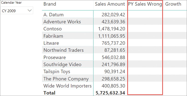
Because the last date is August 15, 2009, moving this date one year back leads to August 15, 2008, which, on purpose, does not exist in Sales[Order Date]. Therefore, SAMEPERIODLASTYEAR returned a blank. Since SAMEPERIODLASTYEAR returned a blank, the second condition inside CALCULATE imposes that the date be less than or equal to blank. There is no date satisfying the condition; therefore, the PY Sales Wrong measure always returns blank.
In the example, we removed one date from Sales to show the issue. In the real world, the problem might happen on any date, if on the corresponding day in the previous year there were no sales. Remember: Time intelligence functions are expected to work on a well-designed date table. Using them on columns from different tables might lead to unexpected results.
Of course, once the overall logic becomes clearer, there can be many ways of expressing the same code. We proposed one version, but you should feel free to experiment.
Finally, scenarios like this one have a much better solution if one can update the data model. Indeed, computing the last date with sales every time a calculation is required and moving it back one year (or by whatever offset is needed) proves to be a tedious, error-prone task. A much better solution is to pre-calculate whether each date should be included in the comparison or not, and consolidate this value directly in the Date table.
One could create a new calculated column in the Date table, which indicates whether a given date should be included in the comparison with the last year or not. In other words, all dates before August 15 have a value of TRUE, whereas all the rows after August 15 have a value of FALSE.
The new calculated column can be authored this way:
'Date'[IsComparable] =
VAR LastDateInSales =
    MAX ( Sales[Order Date] )
VAR LastMonthInSales =
    MONTH ( LastDateInSales )
VAR LastDayInSales =
    DAY ( LastDateInSales )
VAR LastDateCurrentYear =
    DATE ( YEAR ( 'Date'[Date] ), LastMonthInSales, LastDayInSales )
VAR DateIncludedInCompare =
    'Date'[Date] <= LastDateCurrentYear
RETURN
    DateIncludedInCompare
Once the column is in place, the PY Sales measure can be authored much more simply:
PY Sales :=
CALCULATE (
    [Sales Amount],
    SAMEPERIODLASTYEAR ( 'Date'[Date] ),
    'Date'[IsComparable] = TRUE
)
Not only is this code easier to read and debug, it is also way faster than the previous implementation. The reason is that it is no longer necessary to use the complex code required to compute the last date in Sales, move it as a filter on Date, and then apply it to the model. The code is now executed with a simple filter argument of CALCULATE that checks for a Boolean value. The takeaway of this example is that it is possible to move a complex logic for a filter in a calculated column, which is computed during data refresh and not when a user is waiting for the report to come up.
Conclusions
As you have seen, this chapter does not include any new function of the language. Instead, we wanted to show that the same problem can be approached in several different ways. We have not covered the internals of the engine, which is an important topic to introduce optimizations. However, by performing a simple analysis of the code and simulating its behavior, it is oftentimes possible to consider a better formula for the same scenario.
Please remember that this chapter is not about patterns. You can freely use this code in your models, but do not assume that it is the best implementation of the pattern. Our goal was to lead you in thinking about the same scenario in different ways.
As you learn in the next chapters, providing unique patterns in DAX is nearly impossible. The code that runs faster in one data model might not be the top performer in a different data model, or even in the same model with a different data distribution.
If you are serious about optimizing DAX code, then be prepared for a deep dive in the internals of the engine, discovering all the most intricate details of the DAX query engines. This fascinating and complex trip is about to begin, as soon as you turn to the next page.