Chapter 20
Optimizing DAX
This is the last chapter of the book, and it is time to use all the knowledge you have gained so far to explore the most fascinating DAX topic: optimizing formulas. You have learned how the DAX engines work, how to read a query plan, and the internals of the formula engine and of the storage engine. Now all the pieces are in place and you are ready to learn how to use that information to write faster code.
There is one very important warning before approaching this chapter. Do not expect to learn best practices or a simple way to write fast code. Simply stated: There is no way in DAX to write code that is always the fastest. The speed of a DAX formula depends on many factors, the most important of which unfortunately is not in the DAX code itself: It is data distribution. You have already learned that VertiPaq compression strongly depends on data distribution. The size of a column (hence, the speed to scan it) depends on its cardinality: the larger, the slower. Thus, the very same formula might behave differently when executed on one column or another.
You will learn how to measure the speed of a formula, and we will provide you with several examples where rewriting the expression differently leads to a faster execution time. Learn all these examples for what they are—examples that might help you in finding new ideas for your code. Do not take them as golden rules, because they are not.
We are not teaching you rules; we are trying to teach you how to find the best rules in the very specific scenario that is your data model. Be prepared to change them when the data model changes or when you approach a new scenario. Flexibility is key when optimizing DAX code: flexibility, a deep technical knowledge of the engine, and a good amount of creativity, to be prepared to test formulas and expressions that might be not so intuitive.
Finally, all the information we provide in this book is valid at the time of printing. New versions of the engine come on the market every month, and the development team is always working on improving the DAX engine. So be prepared to measure different numbers for the examples of the book in the version of the engine you will be running and be prepared to use different optimization methods if necessary. If one day you measure your code and reach the educated conclusion that “Marco and Alberto are wrong; this code runs much faster than their suggested code,” that will be our brightest day, because we will have been able to teach you all that we know, and you are moving forward in writing better DAX code than ours.
Defining optimization strategies
The optimization process for a DAX query, expression, or measure requires a strategy to reproduce a performance issue, identify the bottleneck, and remove it. Initially, you always observe a slowness in a complex query, but optimizing a complicated expression including several DAX measures is more involved than optimizing one measure at a time. For this reason, the approach we suggest is to isolate the slowest measure or expression first, and optimize it in a simpler query that reproduces the issue with a shorter query plan.
This is a simple to-do list you should follow every time you want to optimize DAX:
Identify a single DAX expression to optimize.
Create a query that reproduces the issue.
Analyze server timings and query plan information.
Identify bottlenecks in the storage engine or formula engine.
Implement changes and rerun the test query.
You can see a more complete description of each of these steps in the following sections.
Identifying a single DAX expression to optimize
If you have already found the slowest measure in your model, you probably can skip this section and move to the following one. However, it is common to get a performance issue in a report that might generate several queries. Each of these queries might include several measures. The first step is to identify a single DAX expression to optimize. Doing this, you reduce the reproduction steps to a single query and possibly to a single measure returned in the result.
A complete refresh of a report in Power BI or Reporting Services or of a Microsoft Excel workbook typically generates several queries in either DAX or MDX (PivotTables and charts in Excel always generate the latter). When a report generates several queries, you have to identify the slowest query first. In Chapter 19, “Analyzing DAX query plans,” you saw how DAX Studio can intercept all the queries sent to the DAX engine and identify the slowest query looking at the largest Duration amount.
If you are using Excel, you can also use a different technique to isolate a query. You can extract the MDX query it generates by using OLAP PivotTable Extensions, a free Excel add-in available at https://olappivottableextensions.github.io/.
Once you extract the slowest DAX or MDX query, you have to further restrict your focus and isolate the DAX expression that is causing the slowness. This way, you will concentrate your efforts on the right area. You can reduce the measures included in a query by modifying and executing the query interactively in DAX Studio.
For example, consider the following table result in Power BI with four expressions (two distinct counts and two measures) grouped by product brand, as shown in Figure 20-1.

The report generates the following DAX query, captured by using DAX Studio:
EVALUATE
TOPN (
    502,
    SUMMARIZECOLUMNS (
        ROLLUPADDISSUBTOTAL ( 'Product'[Brand], "IsGrandTotalRowTotal" ),
        "DistinctCountProductKey", CALCULATE (
            DISTINCTCOUNT ( 'Product'[ProductKey] )
        ),
        "Sales_Amount", 'Sales'[Sales Amount],
        "Margin__", 'Sales'[Margin %],
        "DistinctCountOrder_Number", CALCULATE (
            DISTINCTCOUNT ( 'Sales'[Order Number] )
        )
    ),
    [IsGrandTotalRowTotal], 0,
    'Product'[Brand], 1
)
ORDER BY
    [IsGrandTotalRowTotal] DESC,
    'Product'[Brand]
You should reduce the query by trying one calculation at a time, to locate the slowest one. If you can manipulate the report, you might just include one calculation at a time. By accessing the DAX code, it is enough to comment or remove three of the four columns calculated in the SUMMARIZECOLUMNS function (DistinctCountProductKey, Sales_Amount, Margin__, and DistinctCountOrder_Number), finding the slowest one before proceeding. In this case, the most expensive calculation is the last one. The following query takes up 80% of the time required to compute the original query, meaning that the distinct count over Sales[Order Number] is the most expensive operation in the entire report:
EVALUATE
TOPN (
502,
SUMMARIZECOLUMNS (
ROLLUPADDISSUBTOTAL ( 'Product'[Brand], "IsGrandTotalRowTotal" ),
// "DistinctCountProductKey", CALCULATE (
// DISTINCTCOUNT ( 'Product'[ProductKey] )
// ),
// "Sales_Amount", 'Sales'[Sales Amount],
// "Margin__", 'Sales'[Margin %],
"DistinctCountOrder_Number", CALCULATE (
DISTINCTCOUNT ( 'Sales'[Order Number] )
)
),
[IsGrandTotalRowTotal], 0,
'Product'[Brand], 1
)
ORDER BY
[IsGrandTotalRowTotal] DESC,
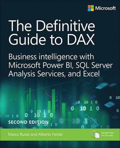
'Product'[Brand]Another example is the following MDX query generated by the pivot table in Excel as seen in Figure 20-2:
SELECT {
    [Measures].[Sales Amount],
    [Measures].[Total Cost],
    [Measures].[Margin],
    [Measures].[Margin %]
  } DIMENSION PROPERTIES PARENT_UNIQUE_NAME, HIERARCHY_UNIQUE_NAME ON COLUMNS,
NON EMPTY HIERARCHIZE(
    DRILLDOWNMEMBER(
        { { DRILLDOWNMEMBER(
                { { DRILLDOWNLEVEL(
                        { [Date].[Calendar].[All] },,, include_calc_members )
                } },
            { [Date].[Calendar].[Year].&[CY 2008] },,, include_calc_members )
        } },
        { [Date].[Calendar].[Quarter].&[Q4-2008] },,, include_calc_members
    )
)
DIMENSION PROPERTIES PARENT_UNIQUE_NAME,HIERARCHY_UNIQUE_NAME ON ROWS
FROM [Model]
CELL PROPERTIES VALUE, FORMAT_STRING, LANGUAGE, BACK_COLOR, FORE_COLOR, FONT_FLAGS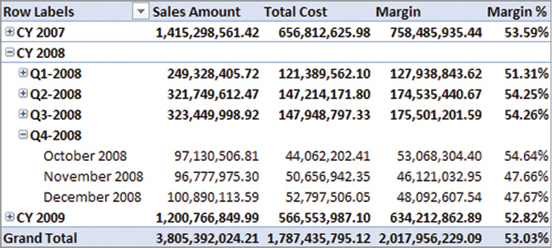
You can reduce the measures either in the pivot table or directly in the MDX code. You can manipulate the MDX code by reducing the list of measures in braces. For example, you reduce the code to only the Sales Amount measure by modifying the list, as in the following initial part of the query:
SELECT
{ [Measures].[Sales Amount] }
DIMENSION PROPERTIES PARENT_UNIQUE_NAME, HIERARCHY_UNIQUE_NAME ON COLUMNS,
...
Regardless of the technique you use, once you identify the DAX expression (or measure) that is responsible for a performance issue, you need a reproduction query to use in DAX Studio.
Creating a reproduction query
The optimization process requires a query that you can execute several times, possibly changing the definition of the measure in order to evaluate different levels of performance.
If you captured a query in DAX or MDX, you already have a good starting point for the reproduction (repro) query. You should try to simplify the query as much as you can, so that it becomes easier to find the bottleneck. You should only keep a complex query structure when it is fundamental in order to observe the performance issue.
Creating a reproduction query in DAX
When a measure is constantly slow, you should be able to create a repro query producing a single value as a result. Using CALCULATE or CALCULATETABLE, you can apply all the filters you need. For example, you can execute the Sales Amount measure for November 2008 using the following code, obtaining the same result ($96,777,975.30) you see in Figure 20-2 for that month:
EVALUATE
{
    CALCULATE (
        [Sales Amount],
        'Date'[Calendar Year] = "CY 2008",
        'Date'[Calendar Year Quarter] = "Q4-2008",
        'Date'[Calendar Year Month] = "November 2008"
    )
}
You can also write the previous query using CALCULATETABLE instead of CALCULATE:
EVALUATE
CALCULATETABLE (
    { [Sales Amount] },
    'Date'[Calendar Year] = "CY 2008",
    'Date'[Calendar Year Quarter] = "Q4-2008",
    'Date'[Calendar Year Month] = "November 2008"
)
The two approaches produce the same result. You should consider CALCULATETABLE when the query you use to test the measure is more complex than a simple table constructor.
Once you have a repro query for a specific measure defined in the data model, you should consider writing the DAX expression of the measure as local in the query, using the MEASURE syntax. For example, you can transform the previous repro query into the following one:
DEFINE
    MEASURE Sales[Sales Amount] =
        SUMX ( Sales, Sales[Quantity] * Sales[Net Price] )
EVALUATE
CALCULATETABLE (
    { [Sales Amount] },
    'Date'[Calendar Year] = "CY 2008",
    'Date'[Calendar Year Quarter] = "Q4-2008",
    'Date'[Calendar Year Month] = "November 2008"
)
At this point, you can apply changes to the DAX expression assigned to the measure directly into the query statement. This way, you do not have to deploy a change to the data model before executing the query again. You can change the query, clear the cache, and run the query in DAX Studio, immediately measuring the performance results of the modified expression.
Creating query measures with DAX Studio
DAX Studio can generate the MEASURE syntax for a measure defined in the model by using the Define Measure context menu item. The latter is available by selecting a measure in the Metadata pane, as shown in Figure 20-3.

If a measure references other measures, all of them should be included as query measures in order to consider any possible change to the repro query. The Define Dependent Measures feature includes the definition of all the measures that are referenced by the selected measure, whereas Define and Expand Measure replaces any measure reference with the corresponding measure expression. For example, consider the following query that just evaluates the Margin % measure:
EVALUATE
{ [Margin %] }
By clicking Define Measure on Margin %, you get the following code, where there are two other references to Sales Amount and Margin measures:
DEFINE
    MEASURE Sales[Margin %] =
        DIVIDE ( [Margin], [Sales Amount] )
EVALUATE
{ [Margin %] }
Instead of repeating the Define Measure action on all the other measures, you can click on Define Dependent Measures on Margin %, obtaining the definition of all the other measures required; this includes Total Cost, which is used in the Margin definition:
DEFINE
    MEASURE Sales[Margin] = [Sales Amount] - [Total Cost]
    MEASURE Sales[Sales Amount] =
        SUMX ( Sales, Sales[Quantity] * Sales[Net Price] )
    MEASURE Sales[Total Cost] =
        SUMX ( Sales, Sales[Quantity] * Sales[Unit Cost] )
    MEASURE Sales[Margin %] =
        DIVIDE ( [Margin], [Sales Amount] )
EVALUATE
{ [Margin %] }
You can also obtain a single DAX expression without measure references by clicking Define and Expand Measure on Margin %:
DEFINE
    MEASURE Sales[Margin %] =
        DIVIDE (
            CALCULATE (
                CALCULATE ( SUMX ( Sales, Sales[Quantity] * Sales[Net Price] ) )
                    - CALCULATE ( SUMX ( Sales, Sales[Quantity] * Sales[Unit Cost] ) )
            ),
            CALCULATE ( SUMX ( Sales, Sales[Quantity] * Sales[Net Price] ) )
        )
EVALUATE
{ [Margin %] }
This latter technique can be useful to quickly evaluate whether a measure includes nested iterators or not, though it could generate very verbose results.
Creating a reproduction query in MDX
In certain conditions, you have to use an MDX query to reproduce a problem that only happens in MDX and not in DAX. The same DAX measure, executed in a DAX or in an MDX query, generates different query plans; it might display a different behavior depending on the language of the query. However in this case too, you can define the DAX measure local to the query. That way, it is more efficient to edit and run again. For instance, you can define the Sales Amount measure local to the MDX query using the WITH MEASURE syntax:
WITH
     MEASURE Sales[Sales Amount] = SUMX ( Sales, Sales[Quantity] * Sales[Unit Price] )
SELECT {
    [Measures].[Sales Amount],
    [Measures].[Total Cost],
    [Measures].[Margin],
    [Measures].[Margin %]
  } DIMENSION PROPERTIES PARENT_UNIQUE_NAME, HIERARCHY_UNIQUE_NAME ON COLUMNS,
NON EMPTY HIERARCHIZE(
    DRILLDOWNMEMBER(
        { { DRILLDOWNMEMBER(
                { { DRILLDOWNLEVEL(
                        { [Date].[Calendar].[All] },,, include_calc_members )
                } },
            { [Date].[Calendar].[Year].&[CY 2008] },,, include_calc_members )
        } },
        { [Date].[Calendar].[Quarter].&[Q4-2008] },,, include_calc_members
    )
)
DIMENSION PROPERTIES PARENT_UNIQUE_NAME,HIERARCHY_UNIQUE_NAME ON ROWS
FROM [Model]
CELL PROPERTIES VALUE, FORMAT_STRING, LANGUAGE, BACK_COLOR, FORE_COLOR, FONT_FLAGS
As you see, in MDX you must use WITH instead of DEFINE, which is how you can rename the syntax generated by DAX Studio if you optimize an MDX query. The syntax after MEASURE is always DAX code, so you will follow the same optimization process for an MDX query. Regardless of the repro query language (either DAX or MDX), you always have a DAX expression to optimize, which you can define within a local MEASURE definition.
Analyzing server timings and query plan information
Once you have a repro query, you run it and collect information about execution time and query plan. You saw in Chapter 19 how to read the information provided by DAX Studio or SQL Server Profiler. In this section, we recap the steps required to analyze a simple query in DAX Studio.
For example, consider the following DAX query:
DEFINE
MEASURE Sales[Sales Amount] =
SUMX ( Sales, Sales[Quantity] * Sales[Unit Price] )
EVALUATE
ADDCOLUMNS (
VALUES ( 'Date'[Calendar Year] ),
"Result", [Sales Amount]
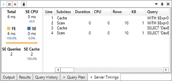
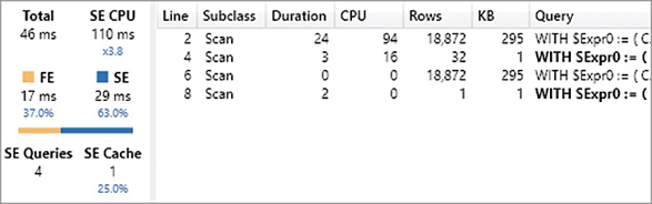
)If you execute this query in DAX Studio after clearing the cache and enabling Query Plan and Server Timings, you obtain a result with one row for each year in the Date table, and the total of Sales Amount for sales made in that year. The starting point for an analysis is always the Server Timings pane, which displays information about the entire query, as shown in Figure 20-4.
Our query returned the result in 25 ms (Total), and it spent 72 percent of this time in the storage engine (SE), whereas the formula engine (FE) only used up 7 ms of the total time. This pane does not provide much information about the formula engine internals, but it is rich in details on storage engine activity. For example, there were two storage engine queries (SE Queries) that consumed a total of 94 ms of processing time (SE CPU). The CPU time can be larger than Duration thanks to the parallelism of the storage engine. Indeed, the engine used 94 ms of logical processors working in parallel, so that the duration time is a fraction of that number. The hardware used in this test had 8 logical processors, and the parallelism degree of this query (ratio between SE CPU and SE) is 5.2. The parallelism cannot be higher than the number of logical processors you have.
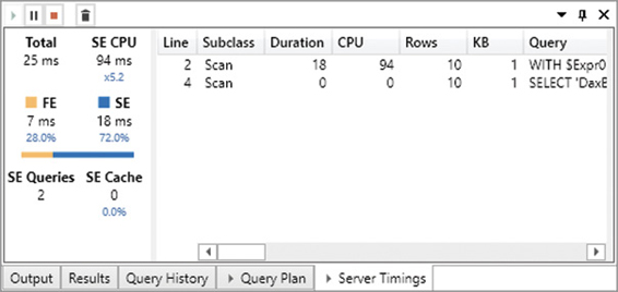
The storage engine queries are available in the list, and you can see that a single storage engine operation (the first one) consumes the entire duration and CPU time. By enabling the display of Internal and Cache subclass events, you can see in Figure 20-5 that the two storage engine queries were actually executed by the storage engine.
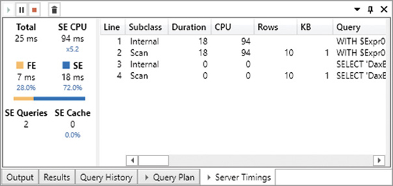
If you execute the same query again without clearing the cache, you see the results in Figure 20-6. Both storage engine queries retrieved the values from the cache (SE cache), and the storage engine queries resolved in the cache are visible in the Subclass column.
Usually, we will use the repro query with a cold cache (clearing the cache before the execution), but in some cases it is important to evaluate whether a given DAX expression can leverage the cache in an upcoming request or not. For this reason, the Cache visualization in DAX Studio is disabled by default, and you enable it on demand.
At this point, you can start looking at the query plans. In Figure 20-7 you see the physical and logical query plans of the query used in the previous example.
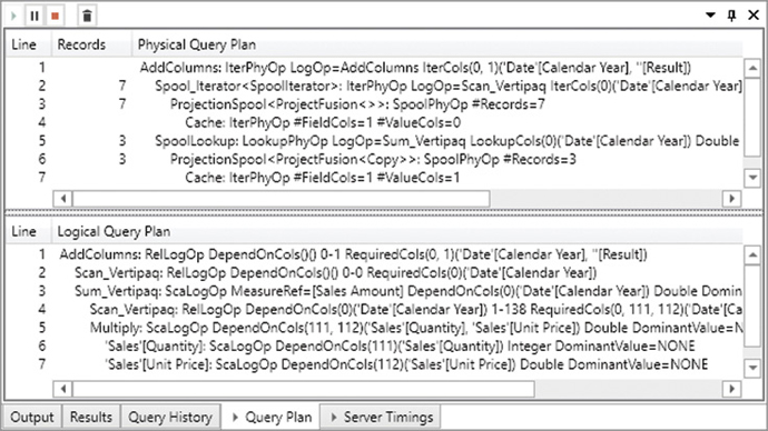
The physical query plan is the one you will use more often. In the query of the previous example, there are two datacaches—one for each storage engine query. Every Cache row in the physical query plan consumes one of the datacaches available. However, there is no simple way to match the correspondence between a query plan operation and a datacache. You can infer the datacache by looking at the columns used in the operations requiring a Cache result (the Spool_Iterator and SpoolLookup rows, in Figure 20-7).
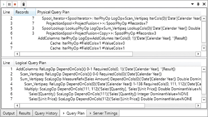
An important piece of information available in the physical query plan is the column showing the number of records processed. As you will see, when optimizing bottlenecks in the formula engine, it might be useful to identify the slowest operation in the formula engine by searching for the line with the largest number of records. You can sort the rows by clicking the Records column header, as you see in Figure 20-8. You restore the original sort order by clicking the Line column header.
Identifying bottlenecks in the storage engine or formula engine
There are many possible optimizations usually available for any query. The first and most important step is to identify whether a query spends most of the time in the formula engine or in the storage engine. A first indication is available in the percentages provided by DAX Studio for FE and SE. Usually, this is a good starting point, but you also have to identify the distribution of the workload in both the formula engine and the storage engine. In complex queries, a large amount of time spent in the storage engine might correspond to a large number of small storage engine queries or to a small number of storage engine queries that concentrate the most of the workload. As you will see, these differences require different approaches in your optimization strategy.
When you identify the execution bottleneck of a query, you should also prioritize the optimization areas. For example, there might be different inefficiencies in the query plan resulting in a large formula engine execution time. You should identify the most important inefficiency and concentrate on that first. If you do not follow this approach, you might end up spending time optimizing an expression that only marginally affects the execution time. Sometimes the more efficient optimizations are simple but hidden in counterintuitive context transitions or in other details of the DAX syntax. You should always measure the execution time before and after each optimization attempt, making sure that you obtain a real advantage and that you are not just applying some optimization pattern you found on the web or in this book without any real benefit.
Finally, remember that even if you have an issue in the formula engine, you should always start your analysis by looking at the storage engine queries. They provide valuable information about the content and size of the datacaches used by the formula engine. Reading the query plan that describes the operations made by the formula engine is a very complex process. It is easier to consider that the formula engine will use the content of datacaches and will have to do all the operations required to produce the result of a DAX query that has not already been produced by the storage engine. This approach is especially efficient for large and complex DAX queries. Indeed, these might generate thousands of lines in a query plan, but a relatively small number of datacaches produced by storage engine queries.
Implementing changes and rerunning the test query
Once the bottlenecks have been identified, the next step is to change the DAX expressions and/or the data model, so that the query plan is more efficient. Running the test query again, it is possible to verify that the improvement is effective, starting the search for the next bottleneck and continuing the loop restarting at the step “Analyzing server timings and query plan information.” This process will continue until the performance is optimal or there are no further possible improvements that are worth the effort.
Optimizing bottlenecks in DAX expressions
A longer execution time in the storage engine is usually the consequence of one or more of the following causes (explained in more detail in Chapter 19):
Longer scan time. Even for a simple aggregation, a DAX query must scan one or more columns. The cost for this scan depends on the size of the column, which depends on the number of unique values and on the data distribution. Different columns in the same table can have very different execution times.
Large cardinality. A large number of unique values in a column affects the DISTINCTCOUNT calculation and the filter arguments of the CALCULATE and CALCULATETABLE functions. A large cardinality can also affect the scan time of a column, but it could be an issue by itself regardless of the column data size.
High frequency of CallbackDataID. A large number of calls made by the storage engine to the formula engine can affect the overall performance of a query.
Large materialization. If a storage engine query produces a large datacache, its generation requires time (allocating and writing RAM). Moreover, its consumption (by the formula engine) is also another potential bottleneck.
In the following sections, you will see several examples of optimization. Starting with the concepts you learned in previous chapters, you will see a typical problem reproduced in a simpler query and optimized.
Optimizing filter conditions
Whenever possible, a filter argument of a CALCULATE/CALCULATETABLE function should always filter columns rather than tables. The DAX engine has improved over the years, and several simple table filters are relatively well optimized in 2019 or newer engine versions. However, expressing a filter condition by columns rather than by tables is always a best practice.
For example, consider the report in Figure 20-9 that compares the total of Sales Amount with the sum of the sales transactions larger than $1,000 (Big Sales Amount) for each product brand.
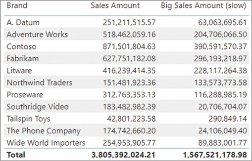
Because the filter condition in the Big Sales Amount measure requires two columns, a trivial way to define the filter is by using a filter over the Sales table. The following query computes just the Big Sales Amount measure in the previous report, generating the server timings results visible in Figure 20-10:
DEFINE
    MEASURE Sales[Big Sales Amount (slow)] =
        CALCULATE (
            [Sales Amount],
            FILTER (
                Sales,
                Sales[Quantity] * Sales[Net Price] > 1000
            )
        )
EVALUATE
SUMMARIZECOLUMNS (
    ROLLUPADDISSUBTOTAL ( 'Product'[Brand], "IsGrandTotalRowTotal" ),
    "Big_Sales_Amount", 'Sales'[Big Sales Amount (slow)]
)
Because FILTER is iterating a table, this query is generating a larger datacache than necessary. The result in Figure 20-9 only displays 11 brands and one additional row for the grand total. Nevertheless, the query plan estimates that the first two datacaches return 3,937 rows, which is the same number as reported also in the Query Plan pane visible in Figure 20-11.
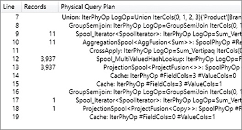
The formula engine receives a much larger datacache than the one required for the query result because there are two additional columns. Indeed, the xmSQL query at line 2 is the following:
WITH
    $Expr0 := ( CAST ( PFCAST ( 'DaxBook Sales'[Quantity] AS  INT ) AS  REAL )
                  * PFCAST ( 'DaxBook Sales'[Net Price] AS  REAL )  )
SELECT
    'DaxBook Product'[Brand],
    'DaxBook Sales'[Quantity],
    'DaxBook Sales'[Net Price],
    SUM ( @$Expr0 )
FROM 'DaxBook Sales'
    LEFT OUTER JOIN 'DaxBook Product'
        ON 'DaxBook Sales'[ProductKey]='DaxBook Product'[ProductKey]
WHERE
  ( COALESCE (  ( CAST ( PFCAST ( 'DaxBook Sales'[Quantity] AS  INT ) AS  REAL )
    * PFCAST ( 'DaxBook Sales'[Net Price] AS  REAL )  )  ) > COALESCE ( 1000.000000 ) );
The structure of the xmSQL query at line 4 in Figure 20-10 is similar to the previous one, just without the SUM aggregation. The presence of a table filter in CALCULATE results in this side effect in the query plan because the semantic of the filter includes all the columns of the Sales expanded table (expanded tables are described in Chapter 14, “Advanced DAX concepts”).
The optimization of the measure only requires a column filter. Because the filter expression uses two columns, a row context requires a table with just those two columns to produce a corresponding and more efficient filter argument to CALCULATE. The following query implements the columns filter adding KEEPFILTERS to keep the same semantic as the previous version, generating the server timings results visible in Figure 20-12:
DEFINE
    MEASURE Sales[Big Sales Amount (fast)] =
        CALCULATE (
            [Sales Amount],
            KEEPFILTERS (
                FILTER (
                    ALL (
                        Sales[Quantity],
                        Sales[Net Price]
                    ),
                    Sales[Quantity] * Sales[Net Price] > 1000
                )
            )
        )
EVALUATE
SUMMARIZECOLUMNS (
    ROLLUPADDISSUBTOTAL ( 'Product'[Brand], "IsGrandTotalRowTotal" ),
    "Big_Sales_Amount", 'Sales'[Big Sales Amount (fast)]
)
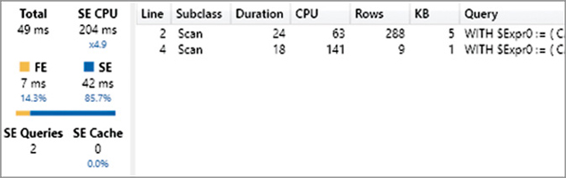
The DAX query runs faster, but what is more important is that there is only one datacache for the rows of the result, excluding the grand total, which still has a separate xmSQL query. The materialization of the datacache at line 2 in Figure 20-12 only returns 14 estimated rows, when there are only 11 in the actual count visible in the Query Plan pane in Figure 20-13.

The reason for this optimization is that the query plan can create a much more efficient calculation in the storage engine without returning additional data to the formula engine because of the semantic required by a table filter. The following is the xmSQL query at line 2 in Figure 20-12:
WITH
    $Expr0 := ( CAST ( PFCAST ( 'DaxBook Sales'[Quantity] AS  INT ) AS  REAL )
                  * PFCAST ( 'DaxBook Sales'[Net Price] AS  REAL )  )
SELECT
    'DaxBook Product'[Brand],
    SUM ( @$Expr0 )
FROM 'DaxBook Sales'
    LEFT OUTER JOIN 'DaxBook Product'
        ON 'DaxBook Sales'[ProductKey]='DaxBook Product'[ProductKey]
WHERE
  ( COALESCE (  ( CAST ( PFCAST ( 'DaxBook Sales'[Quantity] AS  INT ) AS  REAL )
    * PFCAST ( 'DaxBook Sales'[Net Price] AS  REAL )  )  ) > COALESCE ( 1000.000000 ) );
The datacache no longer includes the Quantity and Net Price columns, and its cardinality corresponds to the cardinality of the DAX result. This is an ideal condition for minimal materialization. Keeping the filter conditions using columns rather than tables is an important effort to achieve this goal.
The important takeaway of this section is that you should always pay attention to the rows returned by storage engine queries. When their number is much bigger than the rows included in the result of a DAX query, there might be some overhead caused by the additional work performed by the storage engine to materialize datacaches and by the formula engine to consume such datacaches. Table filters are one of the most common reasons for excessive materialization, though they are not always responsible for bad performance.
![]() Note
Note
When you write a DAX filter, consider the cardinality of the resulting filter. If the cardinality using a table filter is identical to a column filter and the table filter does not expand to other tables, then the table filter can be used safely. For example, there is not usually much difference between filtering a Date table versus the Date[Date] column.
Optimizing context transitions
The storage engine can only compute simple aggregations and simple grouping over columns of the model. Anything else must be computed by the formula engine. Every time there is an iteration and a corresponding context transition, the storage engine materializes a datacache at the granularity level of the iterated table. If the expression computed during the iteration is simple enough to be solved by the storage engine, the performance is typically good. Otherwise, if the expression is too complex, a large materialization and/or a CallbackDataID might occur as we demonstrate in the following example. In these scenarios, simplifying the code by reducing the number of context transitions and by reducing the granularity of the iterated table greatly helps in improving performance. For example, consider a Cashback measure that multiplies the Sales Amount by the Cashback % attribute assigned to each Customer based on an algorithm defined by the marketing department. The report in Figure 20-14 displays the Cashback amount for each country.

The easiest and most intuitive way to create the Cashback measure is also the slowest, which multiplies the Cashback % by the Sales Amount for each customer, summing the result. The following query computes the slowest Cashback measure in the previous report, generating the server timings results visible in Figure 20-15:
DEFINE
    MEASURE Sales[Cashback (slow)] =
        SUMX (
            Customer,
            [Sales Amount] * Customer[Cashback %]
        )
EVALUATE
SUMMARIZECOLUMNS (
    ROLLUPADDISSUBTOTAL ( 'Customer'[Country], "IsGrandTotalRowTotal" ),
    "Cashback", 'Sales'[Cashback (slow)]
)
The queries at lines 2 and 4 of Figure 20-15 compute the result at the Country level, whereas the queries at lines 6 and 8 run the same task for the grand total. We will focus exclusively on the first two storage engine queries. In order to check whether the estimation for the rows materialized is correct, you can look at the query plan in Figure 20-16. This could be surprising, because it seems that a few storage engine queries are not used at all.

The query plan in Figure 20-16 only reports two Cache nodes, which correspond to lines 4 and 8 of the Server Timings pane in Figure 20-15. This is another example of why looking at the query plan could be confusing. The formula engine is actually doing some other work, but the execution within a CallbackDataID is not always reported in the query plan, and this is one of those cases. This is the xmSQL query at line 4 of Figure 20-15, which returns 29 effective rows instead of the estimated 32:
WITH
    $Expr0 := ( [CallbackDataID ( SUMX ( Sales, Sales[Quantity]] * Sales[Net Price]] ) )
                   ] ( PFDATAID ( 'DaxBook Customer'[CustomerKey] ) )
                * PFCAST ( 'DaxBook Customer'[Cashback %] AS  REAL )  )
SELECT
    'DaxBook Customer'[Country],
    SUM ( @$Expr0 )
FROM 'DaxBook Customer';
The DAX code passed to CallbackDataID must be computed for each customer by the formula engine, which receives the CustomerKey as argument. You can see the additional storage engine queries, but the corresponding query plan is not visible in this case. Therefore, we can only imagine what the query plan does by looking at the other storage engine query at line 2 of Figure 20-15:
WITH
    $Expr0 := ( CAST ( PFCAST ( 'DaxBook Sales'[Quantity] AS  INT ) AS  REAL )
              * PFCAST ( 'DaxBook Sales'[Net Price] AS  REAL )  )
SELECT
    'DaxBook Customer'[CustomerKey],
    SUM ( @$Expr0 )
FROM 'DaxBook Sales'
    LEFT OUTER JOIN 'DaxBook Customer'
        ON 'DaxBook Sales'[CustomerKey]='DaxBook Customer'[CustomerKey];
The result of this xmSQL query only contains two columns: the CustomerKey and the result of the Sales Amount measure for that customer. Thus, the formula engine uses the result of this query to provide a result to the CallbackDataID request of the former query.
Once again, instead of trying to describe the exact sequence of operations performed by the engine, it is easier to analyze the result of the storage engine queries, checking whether the materialization is larger than what is required for the query result. In this case the answer is yes: the DAX query returns only 6 visible countries, whereas a total of 29 countries were computed by the formula engine. In any case, there is a huge difference with the materialization of 18,872 customers produced by the latter xmSQL query analyzed. Is it possible to push more workload to the storage engine, aggregating the data by country instead of by customer? The answer is yes, by reducing the number of context transitions. Consider the original Cashback measure: the expression executed in the row context depends on a single column of the Customer table (Cashback %):
Sales[Cashback (slow)] :=
SUMX (
    Customer,
    [Sales Amount] * Customer[Cashback %]
)
Because the Sales Amount measure can be computed for a group of customers that have the same Cashback %, the optimal cardinality for the SUMX iterator is defined by the unique values of the Cashback % column. The following optimized version just replaces the first argument of SUMX using the unique values of Cashback % visible in the filter context:
DEFINE
    MEASURE Sales[Cashback (fast)] =
        SUMX (
            VALUES ( Customer[Cashback %] ),
            [Sales Amount] * Customer[Cashback %]
        )
EVALUATE
SUMMARIZECOLUMNS (
    ROLLUPADDISSUBTOTAL ( 'Customer'[Country], "IsGrandTotalRowTotal" ),
    "Cashback", 'Sales'[Cashback (fast)]
)
This way, the materialization is much smaller, as visible in Figure 20-17. However, even though the number of rows materialized is significantly smaller, the overall execution time is similar if not larger; remember that a difference of a few milliseconds should not be considered relevant.
This time there is a single xmSQL query to compute the amount by country. This is the xmSQL query at line 2 of Figure 20-17:
WITH
$Expr0 := ( CAST ( PFCAST ( 'DaxBook Sales'[Quantity] AS INT ) AS REAL )
* PFCAST ( 'DaxBook Sales'[Net Price] AS REAL ) )
SELECT
'DaxBook Customer'[Country],
'DaxBook Customer'[Cashback %],
SUM ( @$Expr0 )
FROM 'DaxBook Sales'
LEFT OUTER JOIN 'DaxBook Customer'
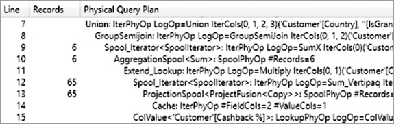
ON 'DaxBook Sales'[CustomerKey]='DaxBook Customer'[CustomerKey];The result of this query contains three columns: Country, Cashback %, and the corresponding Sales Amount value. Thus, the formula engine multiplies Cashback % by Sales Amount for each row, aggregating the rows belonging to the same country. The result presents an estimated count of 288 rows, whereas there are only 65 rows consumed by the formula engine. This is visible in the query plan in Figure 20-18.
Even though it is not evident, this measure is faster than the original measure. Having a smaller footprint in memory, it performs better in more complex reports. This is immediately visible by using a slightly different report like the one in Figure 20-19, grouping the Cashback measure by product brand instead of by customer country.

The following query computes the slowest Cashback measure in the report shown in Figure 20-19, generating the server timings results visible in Figure 20-20:
DEFINE
    MEASURE Sales[Cashback (slow)] =
        SUMX (
            Customer,
            [Sales Amount] * Customer[Cashback %]
        )
EVALUATE
SUMMARIZECOLUMNS (
    ROLLUPADDISSUBTOTAL ( Product[Brand], "IsGrandTotalRowTotal" ),
    "Cashback", 'Sales'[Cashback (slow)]
)
There are a few differences in this query plan, but we focus on the materialization of 192,514 rows produced by the following xmSQL query at line 2 of Figure 20-20:
WITH
    $Expr0 := ( CAST ( PFCAST ( 'DaxBook Sales'[Quantity] AS  INT ) AS  REAL )
              * PFCAST ( 'DaxBook Sales'[Net Price] AS  REAL )  )
SELECT
    'DaxBook Customer'[CustomerKey],
    'DaxBook Product'[Brand],
    SUM ( @$Expr0 )
FROM 'DaxBook Sales'
    LEFT OUTER JOIN 'DaxBook Customer'
        ON 'DaxBook Sales'[CustomerKey]='DaxBook Customer'[CustomerKey]
    LEFT OUTER JOIN 'DaxBook Product'
        ON 'DaxBook Sales'[ProductKey]='DaxBook Product'[ProductKey];
The reason for the larger materialization is that now, the inner calculation computes Sales Amount for each combination of CustomerKey and Brand. The estimated count of 192,514 rows is confirmed by the actual count visible in the query plan in Figure 20-21.
When the test query is using the faster measure, the materialization is much smaller and the query response time is also much faster. The execution of the following DAX query produces the server timings results visible in Figure 20-22:
DEFINE
    MEASURE Sales[Cashback (fast)] =
        SUMX (
            VALUES ( Customer[Cashback %] ),
            [Sales Amount] * Customer[Cashback %]
        )
EVALUATE
SUMMARIZECOLUMNS (
    ROLLUPADDISSUBTOTAL ( Product[Brand], "IsGrandTotalRowTotal" ),
    "Cashback", 'Sales'[Cashback (fast)]
)
The materialization is three orders of magnitude smaller (126 rows instead of 192,000), and the total execution time is 9 times faster than the slow version (it was 415 milliseconds and it is 48 milliseconds with the fast version). Because these differences depend on the cardinality of the report, you should focus on the formula that minimizes the work in the formula engine by computing most of the aggregations in the storage engine. Reducing the number of context transitions is an important step to achieve this goal.
![]() Note
Note
Excessive materialization generated by unnecessary context transitions is the most common performance issue in DAX measures. Using table filters instead of column filters is the second most common performance issue. Therefore, making sure that your DAX measures do not have these two problems should be your priority in an optimization effort. By inspecting the server timings, you should be able to quickly see the symptoms by looking at the materialization size.
Optimizing IF conditions
An IF function is always executed by the formula engine. When there is an IF function within an iteration, there could be a CallbackDataID involved in the execution. Moreover, the engine might evaluate the arguments of the IF regardless of the result of the condition in the first argument. Even though the result is correct, you might pay the full cost of processing all the possible solutions. As usual, there could be different behaviors depending on the version of the DAX engine used.
Optimizing IF in measures
Conditional statements in a measure could trigger a dangerous side effect in the query plan, generating the calculation of every conditional branch regardless of whether it is needed or not. In general, it is a good idea to avoid or at least reduce the number of conditional statements in expressions evaluated for measures, applying filters through the filter context whenever possible.
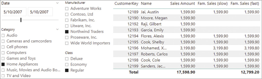
For example, the report in Figure 20-23 displays a Fam. Sales measure that only considers customers with at least one child at home. Because the goal is to display the value for individual customers, the first implementation (slow) does not work for aggregations of two or more customers (Total row is blank), whereas the alternative, faster implementation also works at aggregated levels.
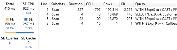
The following query computes the Fam. Sales (slow) measure in a report similar to the one in Figure 20-1. For each customer, an IF statement checks the number of children at home to filter customers classified as a family. The execution of the following DAX query produces the server timings results visible in Figure 20-22:
DEFINE
    MEASURE Sales[Fam. Sales (slow)] =
        VAR ChildrenAtHome = SELECTEDVALUE ( Customer[Children At Home] )
        VAR Result =
            IF (
                ChildrenAtHome > 0,
                [Sales Amount]
            )
        RETURN Result
EVALUATE
CALCULATETABLE (
    SUMMARIZECOLUMNS (
        ROLLUPADDISSUBTOTAL (
            ROLLUPGROUP (
                'Customer'[CustomerKey],
                'Customer'[Name]
            ), "IsGrandTotalRowTotal"
        ),
        "Fam__Sales__slow_", 'Sales'[Fam. Sales (slow)]
    ),
    'Product Category'[Category] = "Home Appliances",
    'Product'[Manufacturer] = "Northwind Traders",
    'Product'[Class] = "Regular",
    DATESBETWEEN (
        'Date'[Date],
        DATE ( 2007, 5, 10 ),
        DATE ( 2007, 5, 10 )
    )
)
ORDER BY
    [IsGrandTotalRowTotal] DESC,
    'Customer'[CustomerKey],
    'Customer'[Name]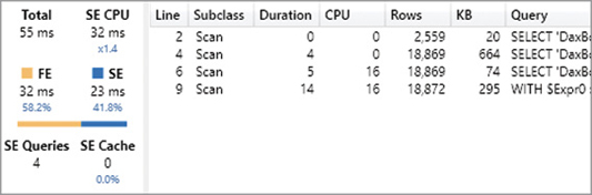
The query is not that slow, but we wanted a query result with a small number or rows because the focus is mainly on the materialization required. We can avoid looking at the query plan, which is already 62 lines long, because the information provided in the Server Timings pane already highlights several facts:
Even though the DAX result only has 7 rows, the rows materialized in three xmSQL queries have more than 18,000 rows, a number close to the number of customers.
The materialization produced by the storage engine query at line 4 in Figure 20-24 includes information about the number of children at home computed for each customer.
The materialization produced by the storage engine query at line 9 in Figure 20-24 includes the Sales Amount measure computed for each customer.
The grand total is not computed by any storage engine query, so it is the formula engine that aggregates the customers to obtain that number.
This is the storage engine query at line 4 in Figure 20-24. It provides the information required by the formula engine to filter customers based on the number of children at home:
SELECT
    'DaxBook Customer'[CustomerKey],
    SUM (  ( PFDATAID ( 'DaxBook Customer'[Children At Home] ) <> 2 )  ),
    MIN ( 'DaxBook Customer'[Children At Home] ),
    MAX ( 'DaxBook Customer'[Children At Home] ),
    COUNT (  )
FROM 'DaxBook Customer';
This result is used as an argument to the following storage engine query at line 9 in Figure 20-24 in order to filter an estimate of 7,368 customers that have at least one child at home:
WITH
$Expr0 := ( CAST ( PFCAST ( 'DaxBook Sales'[Quantity] AS INT ) AS REAL )
* PFCAST ( 'DaxBook Sales'[Net Price] AS REAL ) )
SELECT
'DaxBook Customer'[CustomerKey],
SUM ( @$Expr0 )
FROM 'DaxBook Sales'
LEFT OUTER JOIN 'DaxBook Customer'
ON 'DaxBook Sales'[CustomerKey]='DaxBook Customer'[CustomerKey]
LEFT OUTER JOIN 'DaxBook Date'
ON 'DaxBook Sales'[OrderDateKey]='DaxBook Date'[DateKey]
LEFT OUTER JOIN 'DaxBook Product'
ON 'DaxBook Sales'[ProductKey]='DaxBook Product'[ProductKey]
LEFT OUTER JOIN 'DaxBook Product Subcategory'
ON 'DaxBook Product'[ProductSubcategoryKey]
='DaxBook Product Subcategory'[ProductSubcategoryKey]
LEFT OUTER JOIN 'DaxBook Product Category'
ON 'DaxBook Product Subcategory'[ProductCategoryKey]
='DaxBook Product Category'[ProductCategoryKey]
WHERE
'DaxBook Customer'[CustomerKey]
IN ( 2241, 13407, 5544, 7787, 11090, 7368, 17055, 16636, 1329, 12914..
[7368 total values, not all displayed] )
VAND 'DaxBook Date'[Date] = 39212.000000
VAND 'DaxBook Product'[Manufacturer] = 'Northwind Traders'
VAND 'DaxBook Product'[Class] = 'Regular'
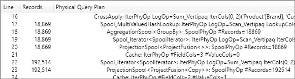
VAND 'DaxBook Product Category'[Category] = 'Home Appliances';The estimated number of rows in this result is wrong, because there are only 7 rows received in the previous storage engine query. This is visible in the query plan; however, it might not be trivial to find the corresponding xmSQL query for each Cache node in the query plan shown in Figure 20-25.

The previous storage engine query receives a filter over the CustomerKey column. The formula engine requires a materialization of such a list of values in CustomerKey in order to provide the corresponding filter in a storage engine query. However, the materialization of a large number of customers in the formula engine is likely to be the bigger cost for this query. The size of this materialization depends on the number of customers. Therefore, a model with hundreds of thousands or millions of customers would make the performance issue evident. In this case you should look at the size of the materialization rather than just the execution time. The latter is still relatively quick. Understanding whether the materialization is efficient is important to create a formula that scales up well with a growing number of rows in the model.
The IF statement in the measure can only be evaluated by the formula engine. This requires either materialization like in this example, or CallbackDataID calls, which we describe later. A better approach is to apply a filter to the filter context using CALCULATE. This removes the need to evaluate an IF condition for every cell of the query result.
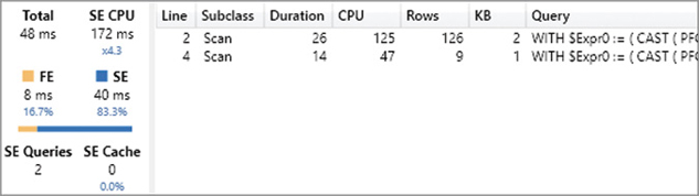
When the test query is using the faster measure, the materialization is much smaller and the query response time is also much shorter. The execution of the following DAX query produces the server timings results visible in Figure 20-26:
DEFINE
    MEASURE Sales[Fam. Sales (fast)] =
        CALCULATE (
            [Sales Amount],
            KEEPFILTERS ( Customer[Children At Home] > 0 )
        )
EVALUATE
CALCULATETABLE (
    SUMMARIZECOLUMNS (
        ROLLUPADDISSUBTOTAL (
            ROLLUPGROUP (
                'Customer'[CustomerKey],
                'Customer'[Name]
            ), "IsGrandTotalRowTotal"
        ),
        "Fam__Sales__fast_", 'Sales'[Fam. Sales (fast)]
    ),
    'Product Category'[Category] = "Home Appliances",
    'Product'[Manufacturer] = "Northwind Traders",
    'Product'[Class] = "Regular",
    DATESBETWEEN (
        'Date'[Date],
        DATE ( 2007, 5, 10 ),
        DATE ( 2007, 5, 10 )
    )
)
ORDER BY
    [IsGrandTotalRowTotal] DESC,
    'Customer'[CustomerKey],
    'Customer'[Name]
Even though there are still four storage engine queries, the query at line 4 in Figure 20-24 is no longer used. The query at line 4 in Figure 20-26 corresponds to the query at line 9 in Figure 20-24. It includes the filter over the number of children, highlighted in the last two lines of the following xmSQL query:
WITH
    $Expr0 := ( CAST ( PFCAST ( 'DaxBook Sales'[Quantity] AS  INT ) AS  REAL )
                 * PFCAST ( 'DaxBook Sales'[Net Price] AS  REAL )  )
SELECT
    'DaxBook Customer'[CustomerKey],
    SUM ( @$Expr0 )
FROM 'DaxBook Sales'
    LEFT OUTER JOIN 'DaxBook Customer'
        ON 'DaxBook Sales'[CustomerKey]='DaxBook Customer'[CustomerKey]
    LEFT OUTER JOIN 'DaxBook Date'
        ON 'DaxBook Sales'[OrderDateKey]='DaxBook Date'[DateKey]
    LEFT OUTER JOIN 'DaxBook Product'
        ON 'DaxBook Sales'[ProductKey]='DaxBook Product'[ProductKey]
    LEFT OUTER JOIN 'DaxBook Product Subcategory'
        ON 'DaxBook Product'[ProductSubcategoryKey]
               ='DaxBook Product Subcategory'[ProductSubcategoryKey]
    LEFT OUTER JOIN 'DaxBook Product Category'
        ON 'DaxBook Product Subcategory'[ProductCategoryKey]
               ='DaxBook Product Category'[ProductCategoryKey]
WHERE
     'DaxBook Date'[Date] = 39212.000000
VAND 'DaxBook Product'[Manufacturer] = 'Northwind Traders'
VAND 'DaxBook Product'[Class] = 'Regular'
VAND 'DaxBook Product Category'[Category] = 'Home Appliances'
VAND ( PFCASTCOALESCE ( 'DaxBook Customer'[Children At Home] AS  INT )
           > COALESCE ( 0 )  );
This different query plan has pros and cons. The advantage is that the formula engine bears a lower workload, not having to transfer the filter of customers back and forth between storage engine queries. The price to pay for this is that the execution of the filters is applied at the storage engine level, which results in an increased cost moving from a former 32 ms of SE CPU time to the current 94 ms of SE CPU time.
Another side effect of the new query plan is the additional storage engine query at line 8 in Figure 20-26; this query computes the aggregation at the grand total without having to perform such aggregation in the formula engine, as was the case in the slower measure. The code is similar to the previous xmSQL query, without the aggregation by CustomerKey.
As a rule of thumb, replacing a conditional statement with a filter argument in CALCULATE is usually a good idea, prioritizing a smaller materialization rather than looking at the execution time for small queries. This way, the expression is usually more scalable with larger data models. However, you should always evaluate the performance in specific conditions, analyzing the metrics provided by DAX Studio using different implementations; you might otherwise choose an implementation that, in a particular scenario, turns out to be slower and not faster.
Choosing between IF and DIVIDE
A very common use of the IF statement is to make sure that an expression is only evaluated with valid arguments. For example, an IF function can validate the denominator of a division to avoid a division by zero. For this specific condition, the DIVIDE function provides a faster alternative. It is interesting to consider why the code is faster by analyzing the different executions with DAX Studio.
The report in Figure 20-27 displays an Average Price measure by customer and brand.

The following query computes the Average Price (slow) measure in the report shown in Figure 20-27. For each combination of product brand and customer, it divides the sales amount by the sum of quantity—only if the latter is not equal to zero. The execution of this DAX query produces the server timings results visible in Figure 20-28:
DEFINE
    MEASURE Sales[Average Price (slow)] =
        VAR Quantity = SUM ( Sales[Quantity] )
        VAR SalesAmount = [Sales Amount]
        VAR Result =
            IF (
                Quantity <> 0,
                SalesAmount / Quantity
            )
        RETURN Result
EVALUATE
TOPN (
    502,
    SUMMARIZECOLUMNS (
        ROLLUPADDISSUBTOTAL (
            ROLLUPGROUP (
                'Customer'[CustomerKey],
                'Product'[Brand]
            ), "IsGrandTotalRowTotal"
        ),
        "Average_Price__slow_", 'Sales'[Average Price (slow)]
    ),
    [IsGrandTotalRowTotal], 0,
    'Customer'[CustomerKey], 1,
    'Product'[Brand], 1
)
ORDER BY
    [IsGrandTotalRowTotal] DESC,
    'Customer'[CustomerKey],
    'Product'[Brand]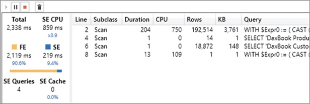
Though the result of the query is limited to 500 rows, the materialization of the datacaches returned by the storage engine queries is much larger. The following xmSQL query is executed at line 2 in Figure 20-28, and returns one row for each combination of customer and brand:
WITH
    $Expr0 := ( CAST ( PFCAST ( 'DaxBook Sales'[Quantity] AS  INT ) AS  REAL )
                  * PFCAST ( 'DaxBook Sales'[Net Price] AS  REAL )  )
SELECT
    'DaxBook Customer'[CustomerKey],
    'DaxBook Product'[Brand],
    SUM ( @$Expr0 ),
    SUM ( 'DaxBook Sales'[Quantity] )
FROM 'DaxBook Sales'
    LEFT OUTER JOIN 'DaxBook Customer'
        ON 'DaxBook Sales'[CustomerKey]='DaxBook Customer'[CustomerKey]
    LEFT OUTER JOIN 'DaxBook Product'
        ON 'DaxBook Sales'[ProductKey]='DaxBook Product'[ProductKey];
The query does not have any filter; therefore, the formula engine evaluates every row returned by this datacache, sorting the result and choosing the first 500 rows to return. This is certainly the most expensive part of the storage engine execution, which consumes 90% of the query duration time. The other three storage engine queries return the list of product brands (line 4), the list of customers (line 6), and the value of sales amount and quantity at the grand total level (line 8). However, these queries are less important in the optimization process. What matters is the formula engine cost required to execute the IF condition on more than 190,000 rows. The query plan resulting from the slow version of the measure has more than 80 lines (not reported here), and it consumes every datacache multiple times. This is a side effect of having different execution branches in an IF statement.
The optimization of the Average Price measure is based on replacing the IF function with DIVIDE. The execution of the following DAX query produces the server timings results visible in Figure 20-29:
DEFINE
    MEASURE Sales[Average Price (fast)] =
        VAR Quantity = SUM ( Sales[Quantity] )
        VAR SalesAmount = [Sales Amount]
        VAR Result =
            DIVIDE (
                SalesAmount,
                Quantity
            )
        RETURN Result
EVALUATE
TOPN (
    502,
    SUMMARIZECOLUMNS (
        ROLLUPADDISSUBTOTAL (
            ROLLUPGROUP (
                'Customer'[CustomerKey],
                'Product'[Brand]
            ), "IsGrandTotalRowTotal"
        ),
        "Average_Price__fast_", 'Sales'[Average Price (fast)]
    ),
    [IsGrandTotalRowTotal], 0,
    'Customer'[CustomerKey], 1,
    'Product'[Brand], 1
)
ORDER BY
    [IsGrandTotalRowTotal] DESC,
    'Customer'[CustomerKey],
    'Product'[Brand]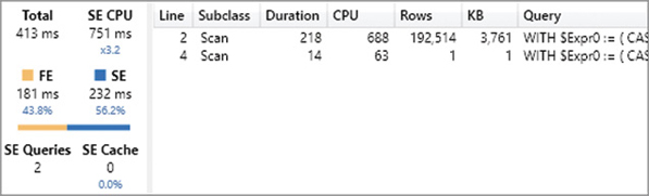
The query now runs in 413 milliseconds, saving more than 80% of the execution time. At first sight, there being only two storage engine queries instead of four might seem like a good reason for the improved performance. However, this is not really the case. Overall, the SE CPU time did not change significantly, and the larger materialization is still there. The optimization is obtained by a shorter and more efficient query plan, which has only 36 lines instead of more than 80 generated by the slower query. In other words, DIVIDE reduces the size and complexity of the query plan, saving time in the formula engine execution by almost one order of magnitude.
Optimizing IF in iterators
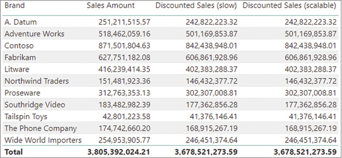
Using the IF statement within a large iterator might create expensive callbacks to the formula engine. For example, consider a Discounted Sales measure that applies a 10% discount to every transaction that has a quantity greater than or equal to 3. The report in Figure 20-30 displays the Discounted Sales amount for each product brand.
The following query computes the slower Discounted Sales measure in the previous report, generating the server timings results visible in Figure 20-31:
DEFINE
    MEASURE Sales[Discounted Sales (slow)] =
        SUMX (
            Sales,
            Sales[Quantity] * Sales[Net Price] * IF (
                    Sales[Quantity] >= 3,
                    .9,
                    1
                )
        )
EVALUATE
SUMMARIZECOLUMNS (
    ROLLUPADDISSUBTOTAL ( 'Product'[Brand], "IsGrandTotalRowTotal" ),
    "Sales_Amount", 'Sales'[Sales Amount],
    "Discounted_Sales__slow_", 'Sales'[Discounted Sales (slow)]
)
ORDER BY
    [IsGrandTotalRowTotal] DESC,
    'Product'[Brand]
The IF statement executed in the SUMX iterator produces two storage engine queries with a CallbackDataID call. The following is the xmSQL query at line 2 of Figure 20-31:
WITH
    $Expr0 := (  ( CAST ( PFCAST ( 'DaxBook Sales'[Quantity] AS  INT ) AS  REAL )
                     * PFCAST ( 'DaxBook Sales'[Net Price] AS  REAL )  )
                     * [CallbackDataID ( IF ( Sales[Quantity]] >= 3, .9, 1 )  ) ]
                         ( PFDATAID ( 'DaxBook Sales'[Quantity] )  )  ) ,
    $Expr1 := ( CAST ( PFCAST ( 'DaxBook Sales'[Quantity] AS  INT ) AS  REAL )
                  * PFCAST ( 'DaxBook Sales'[Net Price] AS  REAL )  )
SELECT
    'DaxBook Product'[Brand],
    SUM ( @$Expr0 ),
    SUM ( @$Expr1 )
FROM 'DaxBook Sales'
    LEFT OUTER JOIN 'DaxBook Product'
        ON 'DaxBook Sales'[ProductKey]='DaxBook Product'[ProductKey];
The presence of a CallbackDataID comes with two consequences: a slower execution time compared to the storage engine performance and the unavailability of the storage engine cache. The datacache must be computed every time and cannot be retrieved from the cache in subsequent requests. The second issue could be more important than the first one, as is the case for this example.
The CallbackDataID can be removed by rewriting the measure in a different way, summing the value of two CALCULATE statements with different filters. For example, the Discounted Sales measure can be rewritten using two CALCULATE functions, one for each percentage, filtering the transactions that share the same multiplicator. The following DAX query implements a version of Discounted Sales that does not rely on any CallbackDataID. The code is longer and requires KEEPFILTERS to provide the same semantic as in the original measure, producing the server timings results visible in Figure 20-32:
DEFINE
    MEASURE Sales[Discounted Sales (scalable)] =
        CALCULATE (
            SUMX (
                Sales,
                Sales[Quantity] * Sales[Net Price]
            ) * .9,
            KEEPFILTERS ( Sales[Quantity] >= 3 )
        ) + CALCULATE (
                SUMX (
                    Sales,
                    Sales[Quantity] * Sales[Net Price]
                ),
                KEEPFILTERS ( NOT ( Sales[Quantity] >= 3 ) )
            )
EVALUATE
SUMMARIZECOLUMNS (
    ROLLUPADDISSUBTOTAL ( 'Product'[Brand], "IsGrandTotalRowTotal" ),
    "Sales_Amount", 'Sales'[Sales Amount],
    "Discounted_Sales__slow_", 'Sales'[Discounted Sales (scalable)]
)
Actually, in this simple query the result is not faster at all. The query required 159 milliseconds instead of the 142 milliseconds of the “slow” version. However, we called this measure “scalable.” Indeed, the important advantage is that a second execution of the last query with a warm cache produces the results visible in Figure 20-33, whereas multiple executions of the query for the “slow” version always produce a result similar to the one shown in Figure 20-31.
The Server Timings in Figure 20-33 show that there is no SE CPU cost after the first execution of the query. This is important when a model is published on a server and many users open the same reports: Users experience a faster response time, and the memory and CPU workload on the server side is reduced. This optimization is particularly relevant in environments with a fixed reserved capacity, such as Power BI Premium and Power BI Report Server.
The rule of thumb is to carefully consider the IF function in the expression of an iterator with a large cardinality because of the possible presence of CallbackDataID in the storage engine queries. The next section includes a deeper discussion on the impact of CallbackDataID, which might be required by many other DAX functions used in iterators.
![]() Note
Note
The SWITCH function in DAX is similar to a series of nested IF functions and can be optimized in a similar way.
Reducing the impact of CallbackDataID
In Chapter 19, you saw that the CallbackDataID function in a storage engine query can have a huge performance impact. This is because it slows down the storage engine execution, and it disables the use of the storage engine cache for the datacache produced. Identifying the CallbackDataID is important because this is often the reason behind a bottleneck in the storage engine, especially for models that only have a few million rows in their largest table (scan time should typically be in the order of magnitude of 10–100 milliseconds).
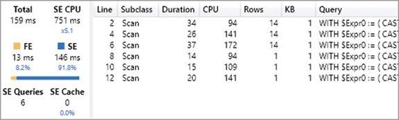
For example, consider the following query where the Rounded Sales measure computes its result rounding Unit Price to the nearest integer. The report in Figure 20-34 displays the Rounded Sales amount for each product brand.
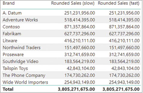
The simpler implementation of Rounded Sales applies the ROUND function to every row of the Sales table. This results in a CallbackDataID call, which slows down the execution, thus lowering performance. The following query computes the slowest Rounded Sales measure in the previous report, generating the server timings results visible in Figure 20-35:
DEFINE
    MEASURE Sales[Rounded Sales (slow)] =
        SUMX (
            Sales,
            Sales[Quantity] * ROUND ( Sales[Net Price], 0 )
        )
EVALUATE
TOPN (
    502,
    SUMMARIZECOLUMNS (
        ROLLUPADDISSUBTOTAL ( 'Product'[Brand], "IsGrandTotalRowTotal" ),
        "Rounded_Sales", 'Sales'[Rounded Sales (slow)]
    ),
    [IsGrandTotalRowTotal], 0,
    'Product'[Brand], 1
)
ORDER BY
    [IsGrandTotalRowTotal] DESC,
    'Product'[Brand]
The two storage engine queries at lines 2 and 4 compute the value for each brand and for the grand total, respectively. This is the xmSQL query at line 2 of Figure 20-35:
WITH
    $Expr0 := ( CAST ( PFCAST ( 'DaxBook Sales'[Quantity] AS  INT ) AS  REAL )
                * [CallbackDataID ( ROUND ( Sales[Net Price]], 0 )  ) ]
                        ( PFDATAID ( 'DaxBook Sales'[Net Price] )  )  )
SELECT
    'DaxBook Product'[Brand],
    SUM ( @$Expr0 )
FROM 'DaxBook Sales'
    LEFT OUTER JOIN 'DaxBook Product'
        ON 'DaxBook Sales'[ProductKey]='DaxBook Product'[ProductKey];
The Sales table contains more than 12 million rows, and each storage engine query computes an equivalent amount of CallbackDataID calls to execute the ROUND function. Indeed, the formula engine executes the ROUND operation to remove the decimal part of the Unit Price value. Based on the Server Timings report, we can estimate that the formula engine executes around 7,000 ROUND functions per millisecond. It is important to keep these numbers in mind, so that you can evaluate whether or not the cardinality of an iterator generating CallbackDataID calls would benefit from some amount of optimization. If the table contained 12,000 rows instead of 12 million rows, the priority would be to optimize something else. However, optimizing the measure in the current model requires reducing the number of CallbackDataID calls.
We aim to reduce the number of CallbackDataID calls by refactoring the measure. By looking at the information provided by VertiPaq Analyzer, we know that the Sales table has more than 12 million rows, whereas the Net Price column in the Sales table has less than 2,500 unique values. Accordingly, the formula can compute the same result by multiplying the rounded value of each unique Unit Price value by the sum of Quantity for all the Sales transaction with the same Unit Price.
![]() Note
Note
You should always use the statistics of your data model during DAX optimization. A quick way to obtain these numbers for a data model is by using VertiPaq Analyzer (http://www.sqlbi.com/tools/vertipaq-analyzer/).
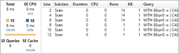
The following optimized version of Rounded Sales materializes up to 2,500 rows computing the sum of Quantity iterating the unique values of Unit Price:
DEFINE
    MEASURE Sales[Rounded Sales (fast)] =
        SUMX (
            VALUES ( Sales[Net Price] ),
            CALCULATE ( SUM ( Sales[Quantity] ) ) * ROUND ( Sales[Net Price], 0 )
        )
EVALUATE
TOPN (
    502,
    SUMMARIZECOLUMNS (
        ROLLUPADDISSUBTOTAL ( 'Product'[Brand], "IsGrandTotalRowTotal" ),
        "Rounded_Sales", 'Sales'[Rounded Sales (fast)]
    ),
    [IsGrandTotalRowTotal], 0,
    'Product'[Brand], 1
)
ORDER BY
    [IsGrandTotalRowTotal] DESC,
    'Product'[Brand]
This way, the formula engine executes the ROUND function using the result of the datacache returning the sum of Quantity for each Net Price. Despite a larger materialization compared to the slow version, the time required to obtain the solution is reduced by almost one order of magnitude. Moreover, the results provided by the storage engine queries can be reused in following executions because the storage engine cache will store the result of xmSQL queries that do not have any CallbackDataID calls.
The following is the xmSQL query at line 2 of Figure 20-36. This query returns the Net Price and the sum of the Quantity for each brand and does not have any CallbackDataID calls:
SELECT
    'DaxBook Product'[Brand],
    'DaxBook Sales'[Net Price],
    SUM ( 'DaxBook Sales'[Quantity] )
FROM 'DaxBook Sales'
    LEFT OUTER JOIN 'DaxBook Product'
        ON 'DaxBook Sales'[ProductKey]='DaxBook Product'[ProductKey];
In this latter version, the rounding is executed by the formula engine and not by the storage engine through the CallbackDataID. Be mindful that a very large number of unique values in Net Price would require a bigger materialization, up to the point where the previous version could be faster with a different data distribution. If Net Price had millions of unique values, a benchmark comparison between the two solutions would be required in order to determine the optimal solution. Moreover, the result could be different depending on the hardware. Rather than assuming that one technique is better than another, you should always evaluate the performance using a real database and not just a sample before making a decision.
Finally, remember that most of the scalar DAX functions that do not aggregate data require a CallbackDataID if executed in an iterator. For example, DATE, VALUE, most of the type conversions, IFERROR, DIVIDE, and all the rounding, mathematical, and date/time functions are only implemented in the formula engine. Most of the time, their presence in an iterator generates a CallbackDataID call. However, you always have to check the xmSQL query to verify whether a CallbackDataID is present or not.
Optimizing nested iterators
Nested iterators in DAX cannot be merged into a single storage engine query. Only the innermost iterator can be executed using a storage engine query, whereas the outer iterators typically require either a larger materialization or additional storage engine queries.
For example, consider another Cashback measure named “Cashback Sim.” that simulates a cashback for each customer using the current price of each product multiplied by the historical quantity and the cashback percentage of each customer. The report in Figure 20-37 displays the Cashback Sim. amount for each country.
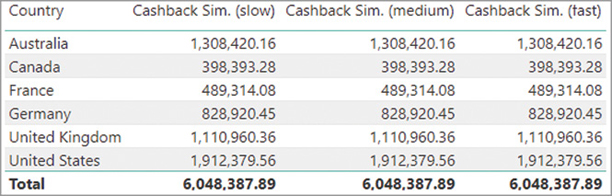
The first and slowest implementation iterates the Customer and Product tables in order to retrieve the cashback percentage of the customer and the current price of the product, respectively. The innermost iterators retrieve the quantity sold for each combination of customer and product, multiplying it by Unit Price and Cashback %. The following query computes the slowest Cashback Sim. measure in the previous report, generating the server timings results visible in Figure 20-38:
DEFINE
    MEASURE Sales[Cashback Sim. (slow)] =
        SUMX (
            Customer,
            SUMX (
                'Product',
                SUMX (
                    RELATEDTABLE ( Sales ),
                    Sales[Quantity] * 'Product'[Unit Price] * Customer[Cashback %]
                )
            )
        )
EVALUATE
TOPN (
    502,
    SUMMARIZECOLUMNS (
        ROLLUPADDISSUBTOTAL ( 'Customer'[Country], "IsGrandTotalRowTotal" ),
        "Cashback Sim. (slow)", 'Sales'[Cashback Sim. (slow)]
    ),
    [IsGrandTotalRowTotal], 0,
    'Customer'[Country], 1
)
ORDER BY
    [IsGrandTotalRowTotal] DESC,
    'Customer'[Country]
The execution cost is split between the storage engine and the formula engine. The former pays a big price to produce a large materialization, whereas the latter spends time consuming that large set of materialized data. The storage engine queries at lines 2 and 10 of Figure 20-38 are identical and materialize the following columns for the entire Sales table: CustomerKey, ProductKey, Quantity, and RowNumber:
SELECT
    'DaxBook Customer'[CustomerKey],
    'DaxBook Product'[ProductKey],
    'DaxBook Sales'[RowNumber],
    'DaxBook Sales'[Quantity]
FROM 'DaxBook Sales'
    LEFT OUTER JOIN 'DaxBook Customer'
        ON 'DaxBook Sales'[CustomerKey]='DaxBook Customer'[CustomerKey]
    LEFT OUTER JOIN 'DaxBook Product'
        ON 'DaxBook Sales'[ProductKey]='DaxBook Product'[ProductKey];
The RowNumber is a special column inaccessible to DAX that is used to uniquely identify a row in a table. These four columns are used in the formula engine to compute the formula in the innermost iterator, which considers the sales for each combination of Customer and Product. The query at line 2 creates the datacache that is also returned at line 10, hitting the cache. The presence of this second storage engine query is caused by the need to compute the grand total in SUMMARIZECOLUMNS. Without the two levels of granularity in the result, half the query plan and half the storage engine queries would not be necessary.
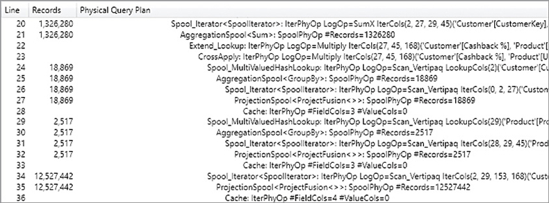
The DAX measure iterates two tables (Customer and Product) producing all the possible combinations. For each combination of customer and product, the innermost SUMX function iterates only the corresponding rows in Sales. The formula also considers the combinations of Customer and Product that do not have any rows in the Sales table, potentially wasting precious CPU time. The query plan shows that there are 2,517 products and 18,869 customers; these are the same numbers estimated for the storage engine queries at lines 4 and 6 in Figure 20-38, respectively. Therefore, the formula engine performs 1,326,280 aggregations of the rows materialized by the Sales table, as shown in the excerpt of the query plan in Figure 20-39. The Records column shows the number of rows iterated by consumed datacaches returned by storage engine queries (see the Cache nodes at lines 28, 33, and 36) or computed by other formula engine operations (see the CrossApply node at line 23).
Although the DAX code iterates the tables, the xmSQL code only retrieves the columns of the tables uniquely representing one row of each table. This reduces the number of columns materialized, even though the cardinality of the tables iterated is larger than necessary. At this point, there are two important considerations:
The cardinality of the iterators is larger than required. Thanks to the context transition, it is possible to reduce the cardinality of the outer iterators; that way, the query context considers all the rows in Sales for a given combination of Unit Price and Cashback %, instead of each combination of product and customer.
Removing nested iterators would produce a better query plan, also removing expensive materialization.
The first consideration should suggest applying the technique previously described to optimize the context transitions. Indeed, the RELATEDTABLE function is like a CALCULATETABLE without filter arguments that only performs a context transition. The first variation to the DAX measure is a “medium” version that iterates the Cashback % and Unit Price columns, instead of iterating by Customer and Product. The semantic of the query is still the same because the innermost expression only depends on these columns:
DEFINE
MEASURE Sales[Cashback Sim. (medium)] =
SUMX (
VALUES ( Customer[Cashback %] ),
SUMX (
VALUES ( 'Product'[Unit Price] ),
SUMX (
RELATEDTABLE ( Sales ),
Sales[Quantity] * 'Product'[Unit Price] * Customer[Cashback %]
)
)
)
EVALUATE
TOPN (
502,
SUMMARIZECOLUMNS (
ROLLUPADDISSUBTOTAL ( 'Customer'[Country], "IsGrandTotalRowTotal" ),
"Cashback Sim. (medium)", 'Sales'[Cashback Sim. (medium)]
),
[IsGrandTotalRowTotal], 0,
'Customer'[Country], 1
)
ORDER BY
[IsGrandTotalRowTotal] DESC,
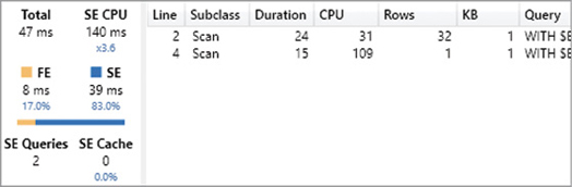
'Customer'[Country]Figure 20-40 shows that the execution of the “medium” version is orders of magnitude faster than the “slow” version, thanks to a smaller granularity and a simpler dependency between tables iterated and columns referenced.

The two storage engine queries provide a result for each of the cardinalities of the result. The following is the storage query at line 2, whereas the similar query at line 4 does not include the Country column and is used for the grand total:
WITH
    $Expr0 := (  ( CAST ( PFCAST ( 'DaxBook Sales'[Quantity] AS  INT ) AS  REAL )
                      * PFCAST ( 'DaxBook Product'[Unit Price] AS  REAL )  )
                      * PFCAST ( 'DaxBook Customer'[Cashback] AS  REAL )  )
SELECT
    'DaxBook Customer'[Country],
    'DaxBook Customer'[Cashback],
    'DaxBook Product'[Unit Price],
    SUM ( @$Expr0 )
FROM 'DaxBook Sales'
    LEFT OUTER JOIN 'DaxBook Customer'
        ON 'DaxBook Sales'[CustomerKey]='DaxBook Customer'[CustomerKey]
    LEFT OUTER JOIN 'DaxBook Product'
        ON 'DaxBook Sales'[ProductKey]='DaxBook Product'[ProductKey];
The “medium” version of the Cashback Sim. measure still contains the same number of nested iterators, potentially considering all the possible combinations between the values of the Unit Price and Cashback % columns. In this simple measure, the query plan is able to establish the dependencies on the Sales table, reducing the calculation to the existing combinations. However, there is an alternative DAX syntax to explicitly instruct the engine to only consider the existing combinations. Instead of using nested iterators, a single iterator over the result of a SUMMARIZE enforces a query plan that does not compute calculations over non-existing combinations. The following version named “improved” could produce a more efficient query plan in complex scenarios, even though in this example it generates the same result and query plan:
MEASURE Sales[Cashback Sim. (improved)] =
    SUMX (
        SUMMARIZE (
            Sales,
            'Product'[Unit Price],
            Customer[Cashback %]
        ),
        CALCULATE ( SUM ( Sales[Quantity] ) )
            * 'Product'[Unit Price] * Customer[Cashback %]
    )
The “medium” and “improved” versions of the Cashback Sim. measure can easily be adapted to use existing measures in the innermost calculations. Indeed, the “improved” version uses a CALCULATE function to compute the sum of Sales[Quantity] for a given combination of Unit Price and Cashback %, just like a measure reference would. You should consider this approach to write efficient code that is easier to maintain. However, a more efficient version is possible by removing any nested iterators.
![]() Note
Note
Note A measure definition often includes aggregation functions such as SUM. With the exception of DISTINCTCOUNT, simple aggregation functions are just a shorter syntax for an iterator. For example, SUM internally invokes SUMX. Hence, a measure reference in an iterator often implies the execution of another nested iterator with a context transition in the middle. When this is required by the nature of the calculation, this is a necessary computational cost. When the nested iterators are additive like the two nested SUMX/SUM of the Cashback Sim. (improved) measure, then a consolidation of the calculation may be considered to optimize the performance; however, this could affect the readability and reusability of the measure.
The following “fast” version of the Cashback Sim. measure optimizes the performance, at the cost of reducing the ability to reuse the business logic of existing measures:
DEFINE
    MEASURE Sales[Cashback Sim. (fast)] =
        SUMX (
            Sales,
            Sales[Quantity]
                * RELATED ( 'Product'[Unit Price] )
                * RELATED ( Customer[Cashback %] )
        )
EVALUATE
TOPN (
    502,
    SUMMARIZECOLUMNS (
        ROLLUPADDISSUBTOTAL ( 'Customer'[Country], "IsGrandTotalRowTotal" ),
        "Cashback Sim. (fast)", 'Sales'[Cashback Sim. (fast)]
    ),
    [IsGrandTotalRowTotal], 0,
    'Customer'[Country], 1
)
ORDER BY
    [IsGrandTotalRowTotal] DESC,
    'Customer'[Country]
Figure 20-41 shows the server timings information of the “fast” version, which saves more than 50% of the execution time compared to the “medium” and “improved” versions.
The measure with a single iterator without context transitions generates the following simple storage engine query, reported at line 2 of Figure 20-41:
WITH
    $Expr0 := (  ( CAST ( PFCAST ( 'DaxBook Sales'[Quantity] AS  INT ) AS  REAL )
                            * PFCAST ( 'DaxBook Product'[Unit Price] AS  REAL )  )
                            * PFCAST ( 'DaxBook Customer'[Cashback] AS  REAL )  )
SELECT
    'DaxBook Customer'[Country],
    SUM ( @$Expr0 )
FROM 'DaxBook Sales'
    LEFT OUTER JOIN 'DaxBook Customer'
        ON 'DaxBook Sales'[CustomerKey]='DaxBook Customer'[CustomerKey]
    LEFT OUTER JOIN 'DaxBook Product'
        ON 'DaxBook Sales'[ProductKey]='DaxBook Product'[ProductKey];
Using the RELATED function does not require any CallbackDataID. Indeed, the only consequence of RELATED is that it enforces a join in the storage engine to enable the access to the related column, which typically has a smaller performance impact compared to a CallbackDataID. However, the “fast” version of the measure is not suggested unless it is critical to obtain the last additional performance improvement and to keep the materialization at a minimal level.
Avoiding table filters for DISTINCTCOUNT
We already mentioned that filter arguments in CALCULATE/CALCULATETABLE functions should be applied to columns instead of tables. The goal of this example on the same topic is to show you an additional query plan pattern that you might find in server timings. A side effect of a table filter is that it requires a large materialization to the storage engine, to enable the formula engine to compute the result. However, for non-additive expressions, the query plan might generate one storage engine query for each element included in the granularity of the result. The DISTINCTCOUNT aggregation is a simple and common example of a non-additive expression.
For example, consider the report in Figure 20-42 that shows the number of customers that made purchases over $1,000 (Customers 1k) for each product name.
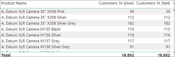
The filter condition in the Customers 1k measure requires two columns. The less efficient way to implement such a condition is by using a filter over the Sales table. The following query computes the Customers 1k measure in the previous report, generating the server timings results visible in Figure 20-43:
DEFINE
    MEASURE Sales[Customers 1k (slow)] =
        CALCULATE (
            DISTINCTCOUNT ( Sales[CustomerKey] ),
            FILTER (
                Sales,
                Sales[Quantity] * Sales[Net Price] > 1000
            )
        )
EVALUATE
TOPN (
    502,
    SUMMARIZECOLUMNS (
        ROLLUPADDISSUBTOTAL ( 'Product'[Product Name], "IsGrandTotalRowTotal" ),
        "Customers_1k__slow_", 'Sales'[Customers 1k (slow)]
    ),
    [IsGrandTotalRowTotal], 0,
    'Product'[Product Name], 1
)
ORDER BY
    [IsGrandTotalRowTotal] DESC,
    'Product'[Product Name]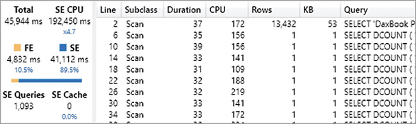
This query generates a large number of storage engine queries—one query for each product included in the result. Because each storage engine query requires 100 to 200 milliseconds, there are a total of several minutes of CPU cost, and the latency is below one minute just because of the parallelism of the storage engine.
The first xmSQL query at line 2 of Figure 20-43 returns the list of product names, including Quantity and Net Price for the sales transactions of that product. Indeed, even though there are only 1,091 products used at least once in the Sales table in transactions with an amount greater than $1,000, the granularity of the datacache is larger because it also includes additional details other than the product name, returning more rows for the same product:
SELECT
    'DaxBook Product'[Product Name],
    'DaxBook Sales'[Quantity],
    'DaxBook Sales'[Net Price]
FROM 'DaxBook Sales'
    LEFT OUTER JOIN 'DaxBook Product'
        ON 'DaxBook Sales'[ProductKey]='DaxBook Product'[ProductKey]
WHERE
    ( COALESCE (  ( CAST ( PFCAST ( 'DaxBook Sales'[Quantity] AS  INT ) AS  REAL )
                             * PFCAST ( 'DaxBook Sales'[Net Price] AS  REAL )  )  )
      > COALESCE ( 1000.000000 )
    );
There are 1,091 xmSQL queries that are very similar to the one at line 6 of Figure 20-43 and return a single value obtained with a distinct count aggregation. In this case, the filter condition has all the combinations of Quantity and Net Price that return a value greater than 1,000 for the Adventure Works 52″ LCD HDTV X790W Silver product:
SELECT
    DCOUNT ( 'DaxBook Sales'[CustomerKey] )
FROM 'DaxBook Sales'
    LEFT OUTER JOIN 'DaxBook Product'
        ON 'DaxBook Sales'[ProductKey]='DaxBook Product'[ProductKey]
WHERE
    ( COALESCE (  ( CAST ( PFCAST ( 'DaxBook Sales'[Quantity] AS  INT ) AS  REAL )
                             * PFCAST ( 'DaxBook Sales'[Net Price] AS  REAL )  )  )
       > COALESCE ( 1000.000000 )
    )
VAND (
        'DaxBook Product'[Product Name],
        'DaxBook Sales'[Quantity],
        'DaxBook Sales'[Net Price] )
    IN {
        ( 'Adventure Works 52" LCD HDTV X790W Silver', 2, 1592.200000 ) ,
        ( 'Adventure Works 52" LCD HDTV X790W Silver', 4, 1432.980000 ) ,
        ( 'Adventure Works 52" LCD HDTV X790W Silver', 1, 1273.760000 ) ,
        ( 'Adventure Works 52" LCD HDTV X790W Silver', 3, 1480.746000 ) ,
        ( 'Adventure Works 52" LCD HDTV X790W Silver', 4, 1512.590000 ) ,
        ( 'Adventure Works 52" LCD HDTV X790W Silver', 3, 1592.200000 ) ,
        ( 'Adventure Works 52" LCD HDTV X790W Silver', 3, 1353.370000 ) ,
        ( 'Adventure Works 52" LCD HDTV X790W Silver', 4, 1273.760000 ) ,
        ( 'Adventure Works 52" LCD HDTV X790W Silver', 1, 1480.746000 ) ,
        ( 'Adventure Works 52" LCD HDTV X790W Silver', 1, 1592.200000 )
    ..[24 total tuples, not all displayed]};
Indeed, the following xmSQL query at line 10 of Figure 20-43 only differs from the latter in the final filter condition, which includes valid combinations of Quantity and Net Price for the Contoso Washer & Dryer 21in E210 Blue product:
SELECT
    DCOUNT ( 'DaxBook Sales'[CustomerKey] )
FROM 'DaxBook Sales'
    LEFT OUTER JOIN 'DaxBook Product'
        ON 'DaxBook Sales'[ProductKey]='DaxBook Product'[ProductKey]
WHERE
    ( COALESCE (  ( CAST ( PFCAST ( 'DaxBook Sales'[Quantity] AS  INT ) AS  REAL )
                             * PFCAST ( 'DaxBook Sales'[Net Price] AS  REAL )  )  )
       > COALESCE ( 1000.000000 )
    )
VAND (
        'DaxBook Product'[Product Name],
        'DaxBook Sales'[Quantity],
        'DaxBook Sales'[Net Price] )
    IN {
         ( 'Contoso Washer & Dryer 21in E210 Blue', 2, 1519.050000 ) ,
         ( 'Contoso Washer & Dryer 21in E210 Blue', 2, 1279.200000 ) ,
         ( 'Contoso Washer & Dryer 21in E210 Blue', 2, 1359.150000 ) ,
         ( 'Contoso Washer & Dryer 21in E210 Blue', 4, 1487.070000 ) ,
         ( 'Contoso Washer & Dryer 21in E210 Blue', 3, 1439.100000 ) ,
         ( 'Contoso Washer & Dryer 21in E210 Blue', 3, 1519.050000 ) ,
         ( 'Contoso Washer & Dryer 21in E210 Blue', 3, 1359.150000 ) ,
         ( 'Contoso Washer & Dryer 21in E210 Blue', 2, 1599.000000 ) ,
         ( 'Contoso Washer & Dryer 21in E210 Blue', 1, 1439.100000 ) ,
         ( 'Contoso Washer & Dryer 21in E210 Blue', 3, 1279.200000 )
    ..[24 total tuples, not all displayed]};
The presence of multiple similar storage engine queries is also visible in the Query Plan pane shown in Figure 20-44. Each row starting at line 15 corresponds to a single datacache with just one column produced by one of the storage engine queries described before.
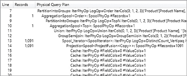
The presence of the table filter applied to the filter context forces a query plan that is not efficient. In this case, a table filter produces multiple storage engine queries instead of a single large materialization. However, the optimization required is always the same: Column filters are better than table filters in CALCULATE and CALCULATETABLE. The optimized version of the Customer 1k measure applies a filter over the two columns Quantity and Net Price, using KEEPFILTERS in order to use the filter semantic of the original measure. The following query produces the Server Timings results visible in Figure 20-45:
DEFINE
    MEASURE Sales[Customers 1k (fast)] =
        CALCULATE (
            DISTINCTCOUNT ( Sales[CustomerKey] ),
            KEEPFILTERS (
                FILTER (
                    ALL (
                        Sales[Quantity],
                        Sales[Net Price]
                    ),
                    Sales[Quantity] * Sales[Net Price] > 1000
                )
            )
        )
EVALUATE
TOPN (
    502,
    SUMMARIZECOLUMNS (
        ROLLUPADDISSUBTOTAL ( 'Product'[Product Name], "IsGrandTotalRowTotal" ),
        "Customers_1k__fast_", 'Sales'[Customers 1k (fast)]
    ),
    [IsGrandTotalRowTotal], 0,
    'Product'[Product Name], 1
)
ORDER BY
    [IsGrandTotalRowTotal] DESC,
    'Product'[Product Name]
The column filter in CALCULATE simplifies the query plan, which now only requires two storage engine queries—one for each granularity level of the result (one product versus total of all products). The following is the xmSQL query at line 4 in Figure 20-45:
SELECT
    'DaxBook Product'[Product Name],
    DCOUNT ( 'DaxBook Sales'[CustomerKey] )
FROM 'DaxBook Sales'
    LEFT OUTER JOIN 'DaxBook Product'
        ON 'DaxBook Sales'[ProductKey]='DaxBook Product'[ProductKey]
WHERE
    ( COALESCE (  ( CAST ( PFCAST ( 'DaxBook Sales'[Quantity] AS  INT ) AS  REAL )
                             * PFCAST ( 'DaxBook Sales'[Net Price] AS  REAL )  )  )
      > COALESCE ( 1000.000000 )
    );
The datacache obtained corresponds to the result of the DAX query. The formula engine does not have to do any further processing. This is an optimal condition for the performance of this query. The lesson here is that the number of storage engine queries can also matter. A large number of storage engine queries might be the result of a bad query plan. Non-additive measures combined with table filters or bidirectional filters could be one of the reasons for this behavior, impacting performance in a negative way.
Avoiding multiple evaluations by using variables
When a DAX expression evaluates the same subexpression multiple times, it is usually a good idea to store the result of the subexpression in a variable, referencing the variable name in following parts of the original DAX expression. The use of variables is a best practice which improves code readability and can provide a better and more efficient query plan—with just some exceptions described later in this section.
For example, the report in Figure 20-46 shows a Sales YOY % measure computing the percentage difference between the value of Sales Amount displayed in the row of the report and the corresponding value in the previous year.
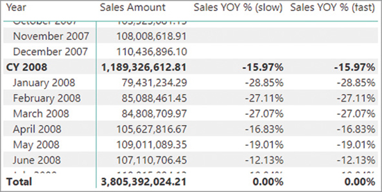
The Sales YOY % measure uses other measures internally. In order to be able to modify each part of the calculation, it is useful to include all the underlying measures using the Define Dependent Measure feature in DAX Studio. The following query computes the original Sales YOY % (slow) measure in the previous report, generating the server timings results visible in Figure 20-47:
DEFINE
    MEASURE Sales[Sales PY] =
        CALCULATE (
            [Sales Amount],
            SAMEPERIODLASTYEAR ( 'Date'[Date] )
        )
    MEASURE Sales[Sales YOY (slow)] =
        IF (
            NOT ISBLANK ( [Sales Amount] ) && NOT ISBLANK ( [Sales PY] ),
            [Sales Amount] - [Sales PY]
        )
    MEASURE Sales[Sales Amount] =
        SUMX (
            Sales,
            Sales[Quantity] * Sales[Net Price]
        )
    MEASURE Sales[Sales YOY % (slow)] =
        DIVIDE (
            [Sales YOY (slow)],
            [Sales PY]
        )
EVALUATE
TOPN (
    502,
    SUMMARIZECOLUMNS (
        ROLLUPADDISSUBTOTAL (
            ROLLUPGROUP (
                'Date'[Calendar Year Month],
                'Date'[Calendar Year Month Number]
            ), "IsGrandTotalRowTotal"
        ),
        "Sales_YOY____slow_", 'Sales'[Sales YOY % (slow)]
    ),
    [IsGrandTotalRowTotal], 0,
    'Date'[Calendar Year Month Number], 1,
    'Date'[Calendar Year Month], 1
)
ORDER BY
    [IsGrandTotalRowTotal] DESC,
    'Date'[Calendar Year Month Number],
    'Date'[Calendar Year Month]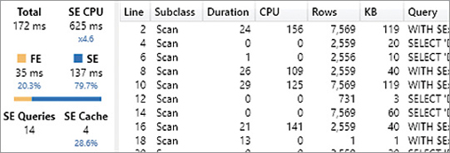
The description of the query plan includes 1,819 rows, not reported here. Moreover, there are four storage engine queries retrieved by the storage engine cache (SE Cache), even though we executed a clear cache command before running the query. This indicates that different parts of the query plan generate different requests for the same storage engine query. Although the cache improves the performance of the storage engine request, the presence of such redundancy in the query plan is an indicator that there is room for further improvements.
When a query plan is so complex and there are many storage engine queries, it is a good idea to review the DAX code and reduce redundant evaluations by using variables. Indeed, redundant evaluations could be responsible for these duplicated requests. In general, the DAX engine should be able to locate similar subexpressions executed within the same filter context, and reuse their results without multiple evaluations. However, the presence of logical conditions such as IF and SWITCH creating different branches of execution can easily stop this internal optimization.
For example, consider the Sales YOY (slow) measure implementation: the Sales Amount and Sales PY measures are executed in different branches of the evaluation. The first argument of the IF function must always be evaluated, whereas the second argument should only be evaluated whenever the first argument evaluates to TRUE. A DAX expression that is present in both the first and the second argument might be evaluated twice in the query plan, which might not consider the result obtained for the first argument as something that can be reused when evaluating the second argument. The technical reasons why this happens and when it turns out to be preferable are outside the scope of this book.
The following excerpt of the previous query highlights the measure references that might be evaluated twice because they are in both the first and the second argument:
MEASURE Sales[Sales YOY (slow)] =
    IF (
        NOT ISBLANK ( [Sales Amount] ) && NOT ISBLANK ( [Sales PY] ),
        [Sales Amount] - [Sales PY]
    )
By storing the values returned by the two measures Sales Amount and Sales PY in two variables, it is possible to instruct the DAX engine to enforce a single evaluation of the two measures before the IF condition, reusing the result in both the first and the second argument. The following excerpt of the Sales YOY (fast) measure shows how to implement this technique in the DAX code:
MEASURE Sales[Sales YOY (fast)] =
    VAR SalesPY = [Sales PY]
    VAR SalesAmount = [Sales Amount]
    RETURN
        IF (
            NOT ISBLANK ( SalesAmount ) && NOT ISBLANK ( SalesPY ),
            SalesAmount - SalesPY
        )
The following query includes a full implementation of the Sales YOY (fast) % measure, which internally relies on Sales YOY (fast) instead of Sales YOY (slow). The execution of the query produces the server timings results visible in Figure 20-48:
DEFINE
    MEASURE Sales[Sales PY] =
        CALCULATE (
            [Sales Amount],
            SAMEPERIODLASTYEAR ( 'Date'[Date] )
        )
    MEASURE Sales[Sales YOY (fast)] =
        VAR SalesPY = [Sales PY]
        VAR SalesAmount = [Sales Amount]
        RETURN
            IF (
                NOT ISBLANK ( SalesAmount ) && NOT ISBLANK ( SalesPY ),
                SalesAmount - SalesPY
            )
    MEASURE Sales[Sales Amount] =
        SUMX (
            Sales,
            Sales[Quantity] * Sales[Net Price]
        )
    MEASURE Sales[Sales YOY % (fast)] =
        DIVIDE (
            [Sales YOY (fast)],
            [Sales PY]
        )
EVALUATE
TOPN (
    502,
    SUMMARIZECOLUMNS (
        ROLLUPADDISSUBTOTAL (
            ROLLUPGROUP (
                'Date'[Calendar Year Month],
                'Date'[Calendar Year Month Number]
            ), "IsGrandTotalRowTotal"
        ),
        "Sales_YOY____fast_", 'Sales'[Sales YOY % (fast)]
    ),
    [IsGrandTotalRowTotal], 0,
    'Date'[Calendar Year Month Number], 1,
    'Date'[Calendar Year Month], 1
)
ORDER BY
    [IsGrandTotalRowTotal] DESC,
    'Date'[Calendar Year Month Number],
    'Date'[Calendar Year Month]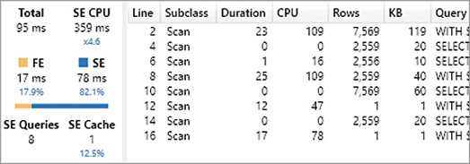
The description of the query plan includes 488 rows (not reported here), reducing the complexity of the query plan by 73%; the previous query plan was 1,819 rows long. The new query plan reduces the cost for the storage engine in terms of both execution time and number of queries, and it also reduces the execution time in the formula engine. Overall, the optimized measure reduces the execution time by about 50%, but the optimization could be even bigger in more complex models and expressions. If the same optimization were applied to nested measures, the improvement might be exponential.
However, pay attention to possible side effects of assigning variables before conditional statements. Only the subexpressions used in the first argument can be assigned to variables defined before an IF or SWITCH statement; otherwise, the effect could be the opposite, enforcing the evaluation of expressions that would otherwise be ignored. You should follow these guidelines:
When the same DAX expression is evaluated multiple times within the same filter context, assign it to a variable and reference the variable instead of the DAX expression.
When a DAX expression is evaluated within the branches of an IF or SWITCH, whenever necessary assign the expression to a variable within the conditional branch.
Do not assign a variable outside an IF or SWITCH statement if the variable is only used within the conditional branch.
The first argument of IF and SWITCH can use variables defined before IF and SWITCH without it affecting performance.
More examples about these guidelines are included in this article: https://www.sqlbi.com/articles/optimizing-if-and-switch-expressions-using-variables/
Conclusions
The lesson in this last chapter (to be honest, in the entire book) is that you must consider all the factors that affect a query plan in order to find the real bottleneck. Looking at the percentages of FE and SE shown in server timings is a good starting point, but you should always investigate the reason behind the numbers. Tools like DAX Studio and VertiPaq Analyzer provide you with the ability to measure the effects of a bad query plan, but these are only clues and pieces of evidence pointing to the reasons for a slow query.
Welcome to the DAX world!