Chapter 3
Using basic table functions
In this chapter, you learn the basic table functions available in DAX. Table functions are regular DAX functions that—instead of returning a single value—return a table. Table functions are useful when writing both DAX queries and many advanced calculations that require iterating over tables. The chapter includes several examples of such calculations.
The goal of this chapter is to introduce the notion of table functions, but not to provide a detailed explanation of all the table functions in DAX. A larger number of table functions is included in Chapter 12, “Working with tables,” and in Chapter 13, “Authoring queries.” Here, we explain the role of most common and important table functions in DAX, and how to use them in common scenarios, including in scalar DAX expressions.
Introducing table functions
Until now, you have seen that a DAX expression usually returns a single value, such as a string or a number. An expression that results in a single value is called a scalar expression. When defining a measure or a calculated column, you always write scalar expressions, as in the following examples:
= 4 + 3
= "DAX is a beautiful language"
= SUM ( Sales[Quantity] )
Indeed, the primary goal of a measure is to produce results that are rendered in a report, in a pivot table, or in a chart. At the end of the day, the source of all these reports is a number—in other words, a scalar expression. Nevertheless, as part of the calculation of a scalar value, you are likely to use tables. For example, a simple iteration like the following uses a table as part of the calculation of the sales amount:
Sales Amount := SUMX ( Sales, Sales[Quantity] * Sales[Net Price] )
In this example, SUMX iterates over the Sales table. Thus, though the result of the full calculation is a scalar value, during the computation the formula scans the Sales table. The same code could iterate the result of a table function, like the following code. This code computes the sales amount only for rows greater than one:
Sales Amount Multiple Items :=
SUMX (
    FILTER (
        Sales,
        Sales[Quantity] > 1
    ),
    Sales[Quantity] * Sales[Net Price]
)
In the example, we use a FILTER function in place of the reference to Sales. Intuitively, FILTER is a function that filters the content of a table based on a condition. We will describe FILTER in full later. For now, it is important to note that whenever you reference the content of a table, you can replace the reference with the result of a table function.
![]() Important
Important
In the previous code you see a filter applied to a sum aggregation. This is not a best practice. In the next chapters, you will learn how to use CALCULATE to implement more flexible and efficient filters. The purpose of the examples in this chapter is not to provide best practices for DAX measures, but rather to explain how table functions work using simple expressions. We will apply these concepts later in more complex scenarios.
Moreover, in Chapter 2, “Introducing DAX,” you learned that you can define variables as part of a DAX expression. There, we used variables to store scalar values. However, variables can store tables too. For example, the previous code could be written this way by using a variable:
Sales Amount Multiple Items :=
VAR
    MultipleItemSales = FILTER ( Sales, Sales[Quantity] > 1 )
RETURN
    SUMX (
        MultipleItemSales,
        Sales[Quantity] * Sales[Unit Price]
    )
MultipleItemSales is a variable that stores a whole table because its expression is a table function. We strongly encourage using variables whenever possible because they make the code easier to read. By simply assigning a name to an expression, you already are documenting your code extremely well.
In a calculated column or inside an iteration, one can also use the RELATEDTABLE function to retrieve all the rows of a related table. For example, the following calculated column in the Product table computes the sales amount of the corresponding product:
'Product'[Product Sales Amount] =
SUMX (
    RELATEDTABLE ( Sales ),
    Sales[Quantity] * Sales[Unit Price]
)
Table functions can be nested too. For example, the following calculated column in the Product table computes the product sales amount considering only sales with a quantity greater than one:
'Product'[Product Sales Amount Multiple Items] =
SUMX (
    FILTER (
        RELATEDTABLE ( Sales ),
        Sales[Quantity] > 1
    ),
    Sales[Quantity] * Sales[Unit Price]
)
In the sample code, RELATEDTABLE is nested inside FILTER. As a rule, when there are nested calls, DAX evaluates the innermost function first and then evaluates the others up to the outermost function.
![]() Note
Note
As you will see later, the execution order of nested calls can be a source of confusion because CALCULATE and CALCULATETABLE have a different order of evaluation from FILTER. In the next section, you learn the behavior of FILTER. You will find the description for CALCULATE and CALCULATETABLE in Chapter 5, “Understanding CALCULATE and CALCULATETABLE.”
In general, we cannot use the result of a table function as the value of a measure or of a calculated column. Both measures and calculated columns require the expression to be a scalar value. Instead, we can assign the result of a table expression to a calculated table. A calculated table is a table whose value is determined by a DAX expression rather than loaded from a data source.
For example, we can create a calculated table containing all the products with a unit price greater than 3,000 by using a table expression like the following:
ExpensiveProducts =
FILTER (
    'Product',
    'Product'[Unit Price] > 3000
)
Calculated tables are available in Power BI and Analysis Services, but not in Power Pivot for Excel (as of 2019). The more you use table functions, the more you will use them to create more complex data models by using calculated tables and/or complex table expressions inside your measures.
Introducing EVALUATE syntax
Query tools such as DAX Studio are useful to author complex table expressions. In that case, a common statement used to inspect the result of a table expression is EVALUATE:
EVALUATE
FILTER (
    'Product',
    'Product'[Unit Price] > 3000
)
One can execute the preceding DAX query in any tool that executes DAX queries (DAX Studio, Microsoft Excel, SQL Server Management Studio, Reporting Services, and so on). A DAX query is a DAX expression that returns a table, used with the EVALUATE statement. EVALUATE has a complex syntax, which we fully cover in Chapter 13. Here we only introduce the more commonly used EVALUATE syntax, which is as follows:
[DEFINE { MEASURE <tableName>[<name>] = <expression> }]
EVALUATE <table>
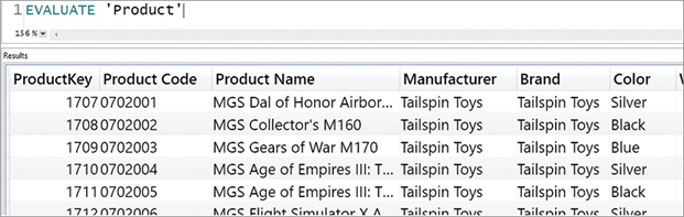
[ORDER BY {<expression> [{ASC | DESC}]} [, ...]]The initial DEFINE MEASURE part can be useful to define measures that are local to the query. It becomes useful when we are debugging formulas because we can define a local measure, test it, and then deploy the code in the model once it behaves as expected. Most of the syntax is optional. Indeed, the simplest query one can author retrieves all the rows and columns from an existing table, as shown in Figure 3-1:
EVALUATE 'Product'
The ORDER BY clause controls the sort order:
EVALUATE
FILTER (
    'Product',
    'Product'[Unit Price] > 3000
)
ORDER BY
    'Product'[Color],
    'Product'[Brand] ASC,
'Product'[Class] DESC![]() Note
Note
Please note that the Sort By Column property defined in a model does not affect the sort order in a DAX query. The sort order specified by EVALUATE can only use columns included in the result. Thus, a client that generates a dynamic DAX query should read the Sort By Column property in a model’s metadata, include the column for the sort order in the query, and then generate a corresponding ORDER BY condition.
EVALUATE is not a powerful statement by itself. The power of querying with DAX comes from the power of using the many DAX table functions that are available in the language. In the next sections, you learn how to create advanced calculations by using and combining different table functions.
Understanding FILTER
Now that we have introduced what table functions are, it is time to describe in full the basic table functions. Indeed, by combining and nesting the basic functions, you can already compute many powerful expressions. The first function you learn is FILTER. The syntax of FILTER is the following:
FILTER ( <table>, <condition> )
FILTER receives a table and a logical condition as parameters. As a result, FILTER returns all the rows satisfying the condition. FILTER is both a table function and an iterator at the same time. In order to return a result, it scans the table evaluating the condition on a row-by-row basis. In other words, it iterates the table.
For example, the following calculated table returns the Fabrikam products (Fabrikam being a brand).
FabrikamProducts =
FILTER (
    'Product',
    'Product'[Brand] = "Fabrikam"
)
FILTER is often used to reduce the number of rows in iterations. For example, if a developer wants to compute the sales of red products, they can author a measure like the following one:
RedSales :=
SUMX (
    FILTER (
        Sales,
        RELATED ( 'Product'[Color] ) = "Red"
    ),
    Sales[Quantity] * Sales[Net Price]
)
You can see the result in Figure 3-2, along with the total sales.
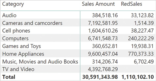
The RedSales measure iterated over a subset of the Sales table—namely the set of sales that are related to a red product. FILTER adds a condition to the existing conditions. For example, RedSales in the Audio row shows the sales of products that are both of Audio category and of Red color.
It is possible to nest FILTER in another FILTER function. In general, nesting two filters produces the same result as combining the conditions of the two FILTER functions with an AND function. In other words, the following two queries produce the same result:
FabrikamHighMarginProducts =
FILTER (
    FILTER (
        'Product',
        'Product'[Brand] = "Fabrikam"
    ),
    'Product'[Unit Price] > 'Product'[Unit Cost] * 3
)

FabrikamHighMarginProducts =
FILTER (
    'Product',
    AND (
        'Product'[Brand] = "Fabrikam",
        'Product'[Unit Price] > 'Product'[Unit Cost] * 3
    )
)
However, performance might be different on large tables depending on the selectivity of the conditions. If one condition is more selective than the other, applying the most selective condition first by using a nested FILTER function is considered best practice.
For example, if there are many products with the Fabrikam brand, but few products priced at three times their cost, then the following query applies the filter over Unit Price and Unit Cost in the innermost FILTER. By doing so, the formula applies the most restrictive filter first, in order to reduce the number of iterations needed to check for the brand:
FabrikamHighMarginProducts =
FILTER (
    FILTER (
        'Product',
        'Product'[Unit Price] > 'Product'[Unit Cost] * 3
    ),
    'Product'[Brand] = "Fabrikam"
)
Using FILTER, a developer can often produce code that is easier to read and to maintain over time. For example, imagine you need to compute the number of red products. Without using table functions, one possible implementation might be the following:
NumOfRedProducts :=
SUMX (
    'Product',
    IF ( 'Product'[Color] = "Red", 1, 0 )
)
The inner IF returns either 1 or 0 depending on the color of the product, and summing this expression returns the number of red products. Although it works, this code is somewhat tricky. A better implementation of the same measure is the following:
NumOfRedProducts :=
COUNTROWS (
    FILTER ( 'Product', 'Product'[Color] = "Red" )
)
This latter expression better shows what the developer wanted to obtain. Moreover, not only is the code easier to read for a human being, but the DAX optimizer is also better able to understand the developer’s intention. Therefore, the optimizer produces a better query plan, leading in turn to better performance.
Introducing ALL and ALLEXCEPT
In the previous section you learned FILTER, which is a useful function whenever we want to restrict the number of rows in a table. Sometimes we want to do the opposite; that is, we want to extend the number of rows to consider for a certain calculation. In that case, DAX offers a set of functions designed for that purpose: ALL, ALLEXCEPT, ALLCROSSFILTERED, ALLNOBLANKROW, and ALLSELECTED. In this section, you learn ALL and ALLEXCEPT, whereas the latter two are described later in this chapter and ALLCROSSFILTERD is introduced in Chapter 14, “Advanced DAX concepts.”
ALL returns all the rows of a table or all the values of one or more columns, depending on the parameters used. For example, the following DAX expression returns a ProductCopy calculated table with a copy of all the rows in the Product table:
ProductCopy = ALL ( 'Product' )
![]() Note
Note
ALL is not necessary in a calculated table because there are no report filters influencing it. However, ALL is useful in measures, as shown in the next examples.
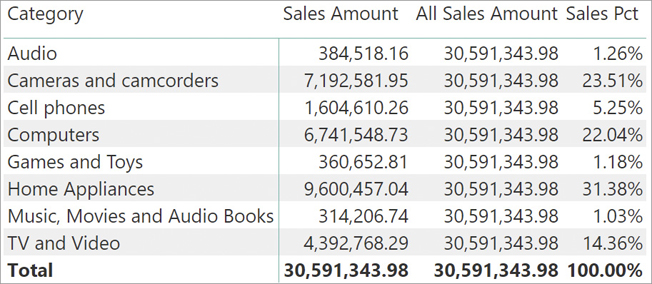
ALL is extremely useful whenever we need to compute percentages or ratios because it ignores the filters automatically introduced by a report. Imagine we need a report like the one in Figure 3-3, which shows on the same row both the sales amount and the percentage of the given amount against the grand total.
The Sales Amount measure computes a value by iterating over the Sales table and performing the multiplication of Sales[Quantity] by Sales[Net Price]:
Sales Amount :=
SUMX (
    Sales,
    Sales[Quantity] * Sales[Net Price]
)
To compute the percentage, we divide the sales amount by the grand total. Thus, the formula must compute the grand total of sales even when the report is deliberately filtering one given category. This can be obtained by using the ALL function. Indeed, the following measure produces the total of all sales, no matter what filter is being applied to the report:
All Sales Amount :=
SUMX (
    ALL ( Sales ),
    Sales[Quantity] * Sales[Net Price]
)
In the formula we replaced the reference to Sales with ALL ( Sales ), making good use of the ALL function. At this point, we can compute the percentage by performing a simple division:
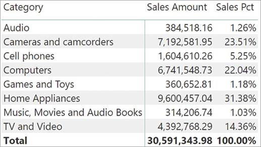
Sales Pct := DIVIDE ( [Sales Amount], [All Sales Amount] )
Figure 3-4 shows the result of the three measures together.
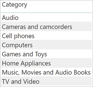
The parameter of ALL cannot be a table expression. It needs to be either a table name or a list of column names. You have already learned what ALL does with a table. What is its result if we use a column instead? In that case, ALL returns all the distinct values of the column in the entire table. The Categories calculated table is obtained from the Category column of the Product table:
Categories = ALL ( 'Product'[Category] )
Figure 3-5 shows the result of the Categories calculated table.
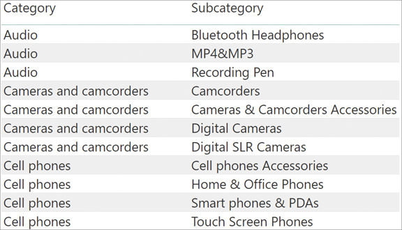
We can specify multiple columns from the same table in the parameters of the ALL function. In that case, ALL returns all the existing combinations of values in those columns. For example, we can obtain the list of all categories and subcategories by adding the Product[Subcategory] column to the list of values, obtaining the result shown in Figure 3-6:
Categories =
ALL (
    'Product'[Category],
    'Product'[Subcategory]
)
Throughout all its variations, ALL ignores any existing filter in order to produce a result. We can use ALL as an argument of an iteration function, such as SUMX and FILTER, or as a filter argument in a CALCULATE function. You learn the CALCULATE function in Chapter 5.
If we want to include most, but not all the columns of a table in an ALL function call, we can use ALLEXCEPT instead. The syntax of ALLEXCEPT requires a table followed by the columns we want to exclude. As a result, ALLEXCEPT returns a table with a unique list of existing combinations of values in the other columns of the table.
ALLEXCEPT is a way to write a DAX expression that will automatically include in the result any additional columns that could appear in the table in the future. For example, if we have a Product table with five columns (ProductKey, Product Name, Brand, Class, Color), the following two expressions produce the same result:
ALL ( 'Product'[Product Name], 'Product'[Brand], 'Product'[Class] )
ALLEXCEPT ( 'Product', 'Product'[ProductKey], 'Product'[Color] )
However, if we later add the two columns Product[Unit Cost] and Product[Unit Price], then the result of ALL will ignore them, whereas ALLEXCEPT will return the equivalent of:
ALL (
    'Product'[Product Name],
    'Product'[Brand],
    'Product'[Class],
    'Product'[Unit Cost],
    'Product'[Unit Price]
)
In other words, with ALL we declare the columns we want, whereas with ALLEXCEPT we declare the columns that we want to remove from the result. ALLEXCEPT is mainly useful as a parameter of CALCULATE in advanced calculations, and it is seldomly adopted with simpler formulas. Thus, even if we included its description here for completeness, it will become useful only later in the learning path.
BestCategories =
VAR Subcategories =
    ALL ( 'Product'[Category], 'Product'[Subcategory] )
VAR AverageSales =
    AVERAGEX (
        Subcategories,
        SUMX ( RELATEDTABLE ( Sales ), Sales[Quantity] * Sales[Net Price] )
    )
VAR TopCategories =
    FILTER (
        Subcategories,
        VAR SalesOfCategory =
            SUMX ( RELATEDTABLE ( Sales ), Sales[Quantity] * Sales[Net Price] )
        RETURN
            SalesOfCategory >= AverageSales * 2
    )
RETURN
    TopCategories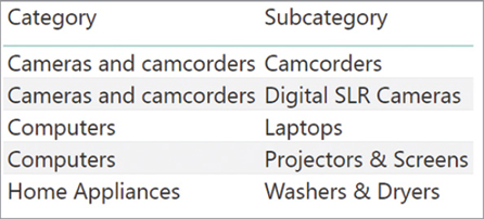
Understanding VALUES, DISTINCT, and the blank row
In the previous section, you saw that ALL used with one column returns a table with all its unique values. DAX provides two other similar functions that return a list of unique values for a column: VALUES and DISTINCT. These two functions look almost identical, the only difference being in how they handle the blank row that might exist in a table. You will learn about the optional blank row later in this section; for now let us focus on what these two functions perform.
ALL always returns all the distinct values of a column. On the other hand, VALUES returns only the distinct visible values. You can appreciate the difference between the two behaviors by looking at the two following measures:
NumOfAllColors := COUNTROWS ( ALL ( 'Product'[Color] ) )
NumOfColors := COUNTROWS ( VALUES ( 'Product'[Color] ) )
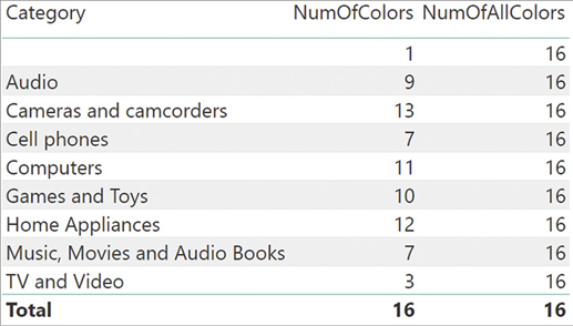
NumOfAllColors counts all the colors of the Product table, whereas NumOfColors counts only the ones that—given the filter in the report—are visible. The result of these two measures, sliced by category, is visible in Figure 3-8.

Because the report slices by category, each given category contains products with some, but not all, the colors. VALUES returns the distinct values of a column evaluated in the current filter. If we use VALUES or DISTINCT in a calculated column or in a calculated table, then their behavior is identical to that of ALL because there is no active filter. On the other hand, when used in a measure, these two functions compute their result considering the existing filters, whereas ALL ignores any filter.
As you read earlier, the two functions are nearly identical. It is now important to understand why VALUES and DISTINCT are two variations of the same behavior. The difference is the way they consider the presence of a blank row in the table. First, we need to understand how come a blank row might appear in our table if we did not explicitly create a blank row.
The fact is that the engine automatically creates a blank row in any table that is on the one-side of a relationship in case the relationship is invalid. To demonstrate the behavior, we removed all the silver-colored products from the Product table. Since there were 16 distinct colors initially and we removed one color, one would expect the total number of colors to be 15. Instead, the report in Figure 3-9 shows something unexpected: NumOfAllColors is still 16 and the report shows a new row at the top, with no name.
Because Product is on the one-side of a relationship with Sales, for each row in the Sales table there is a related row in the Product table. Nevertheless, because we deliberately removed all the products with one color, there are now many rows in Sales that no longer have a valid relationship with the Product table. Be mindful, we did not remove any row from Sales; we removed a color with the intent of breaking the relationship.
To guarantee that these rows are considered in all the calculations, the engine automatically added to the Product table a row containing blank in all its columns. All the orphaned rows in Sales are linked to this newly introduced blank row.
![]() Important
Important
Only one blank row is added to the Product table, despite the fact that multiple different products referenced in the Sales table no longer have a corresponding ProductKey in the Product table.
Indeed, in Figure 3-9 you can see that the first row shows a blank for the Category and accounts for one color. The number comes from a row containing blank in the category, blank in the color, and blank in all the columns of the table. You will not see the row if you inspect the table because it is an automatic row created during the loading of the data model. If, at some point, the relationship becomes valid again—if you were to add the silver products back—then the blank row will disappear from the table.
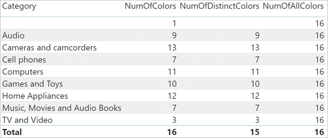
Certain functions in DAX consider the blank row as part of their result, whereas others do not. Specifically, VALUES considers the blank row as a valid row, and it returns it. On the other hand, DISTINCT does not return it. You can appreciate the difference by looking at the following new measure, which counts the DISTINCT colors instead of VALUES:
NumOfDistinctColors := COUNTROWS ( DISTINCT ( 'Product'[Color] ) )
The result is visible in Figure 3-10.
A well-designed model should not present any invalid relationships. Thus, if your model is perfect, then the two functions always return the same values. Nevertheless, when dealing with invalid relationships, you need to be aware of this behavior because otherwise you might end up writing incorrect calculations. For example, imagine that we want to compute the average sales per product. A possible solution is to compute the total sales and divide that by the number of products, by using this code:
AvgSalesPerProduct :=
DIVIDE (
    SUMX (
        Sales,
        Sales[Quantity] * Sales[Net Price]
    ),
    COUNTROWS (
        VALUES ( 'Product'[Product Code] )
    )
)
The result is visible in Figure 3-11. It is obviously wrong because the first row is a huge, meaningless number.

The number shown in the first row, where Category is blank, corresponds to the sales of all the silver products—which no longer exist in the Product table. This blank row associates all the products that were silver and are no longer in the Product table. The numerator of DIVIDE considers all the sales of silver products. The denominator of DIVIDE counts a single blank row returned by VALUES. Thus, a single non-existing product (the blank row) is cumulating the sales of many other products referenced in Sales and not available in the Product table, leading to a huge number. Here, the problem is the invalid relationship, not the formula by itself. Indeed, no matter what formula we create, there are many sales of products in the Sales table for which the database has no information. Nevertheless, it is useful to look at how different formulations of the same calculation return different results. Consider these two other variations:
AvgSalesPerDistinctProduct :=
DIVIDE (
    SUMX ( Sales, Sales[Quantity] * Sales[Net Price] ),
    COUNTROWS ( DISTINCT ( 'Product'[Product Code] ) )
)

AvgSalesPerDistinctKey :=
DIVIDE (
    SUMX ( Sales, Sales[Quantity] * Sales[Net Price] ),
    COUNTROWS ( VALUES ( Sales[ProductKey] ) )
)
In the first variation, we used DISTINCT instead of VALUES. As a result, COUNTROWS returns a blank and the result will be a blank. In the second variation, we still used VALUES, but this time we are counting the number of Sales[ProductKey]. Keep in mind that there are many different Sales[ProductKey] values, all related to the same blank row. The result is visible in Figure 3-12.
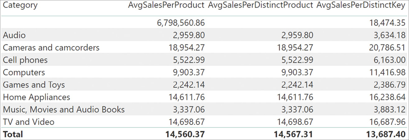
It is interesting to note that AvgSalesPerDistinctKey is the only correct calculation. Since we sliced by Category, each category had a different number of invalid product keys—all of which collapsed to the single blank row.
However, the correct approach should be to fix the relationship so that no sale is orphaned of its product. The golden rule is to not have any invalid relationships in the model. If, for any reason, you have invalid relationships, then you need to be extremely cautious in how you handle the blank row, as well as how its presence might affect your calculations.
As a final note, consider that the ALL function always returns the blank row, if present. In case you need to remove the blank row from the result, then ALLNOBLANKROW is the function you will want to use.
Later, you will see that VALUES and DISTINCT are often used as a parameter of iterator functions. There are no differences in their results whenever the relationships are valid. In such a case, when you iterate over the values of a column, you need to consider the blank row as a valid row, in order to make sure that you iterate all the possible values. As a rule of thumb, VALUES should be your default choice, only leaving DISTINCT to cases when you want to explicitly exclude the possible blank value. Later in this book, you will also learn how to leverage DISTINCT instead of VALUES to avoid circular dependencies. We will cover it in Chapter 15, “Advanced relationships handling.”
VALUES and DISTINCT also accept a table as an argument. In that case, they exhibit different behaviors:
DISTINCT returns the distinct values of the table, not considering the blank row. Thus, duplicated rows are removed from the result.
VALUES returns all the rows of the table, without removing duplicates, plus the additional blank row if present. Duplicated rows, in this case, are kept untouched.
Using tables as scalar values
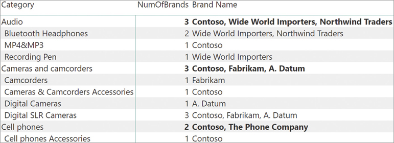
Although VALUES is a table function, we will often use it to compute scalar values because of a special feature in DAX: a table with a single row and a single column can be used as if it were a scalar value. Imagine we produce a report like the one in Figure 3-13, reporting the number of brands sliced by category and subcategory.

One might also want to see the names of the brands beside their number. One possible solution is to use VALUES to retrieve the different brands and, instead of counting them, return their value. This is possible only in the special case when there is only one value for the brand. Indeed, in that case it is possible to return the result of VALUES and DAX automatically converts it into a scalar value. To make sure that there is only one brand, one needs to protect the code with an IF statement:
Brand Name :=
IF (
    COUNTROWS ( VALUES ( Product[Brand] ) ) = 1,
    VALUES ( Product[Brand] )
)
The result is visible in Figure 3-14. When the Brand Name column contains a blank, it means that there are two or more different brands.

The Brand Name measure uses COUNTROWS to check whether the Color column of the Products table only has one value selected. Because this pattern is frequently used in DAX code, there is a simpler function that checks whether a column only has one visible value: HASONEVALUE. The following is a better implementation of the Brand Name measure, based on HASONEVALUE:
Brand Name :=
IF (
    HASONEVALUE ( 'Product'[Brand] ),
    VALUES ( 'Product'[Brand] )
)
Moreover, to make the lives of developers easier, DAX also offers a function that automatically checks if a column contains a single value and, if so, it returns the value as a scalar. In case there are multiple values, it is also possible to define a default value to be returned. That function is SELECTEDVALUE. The previous measure can also be defined as
Brand Name := SELECTEDVALUE ( 'Product'[Brand] )
By including the second optional argument, one can provide a message stating that the result contains multiple results:
Brand Name := SELECTEDVALUE ( 'Product'[Brand], "Multiple brands" )
The result of this latest measure is visible in Figure 3-15.

What if, instead of returning a message like “Multiple brands,” one wants to list all the brands? In that case, an option is to iterate over the VALUES of Product[Brand] and use the CONCATENATEX function, which produces a good result even if there are multiple values:
[Brand Name] :=
CONCATENATEX (
    VALUES ( 'Product'[Brand] ),
    'Product'[Brand],
    ", "
)
Now the result contains the different brands separated by a comma instead of the generic message, as shown in Figure 3-16.
Introducing ALLSELECTED
The last table function that belongs to the set of basic table functions is ALLSELECTED. Actually, ALLSELECTED is a very complex table function—probably the most complex table function in DAX. In Chapter 14, we will uncover all the secrets of ALLSELECTED. Nevertheless, ALLSELECTED is useful even in its basic implementation. For that reason, it is worth mentioning in this introductory chapter.
ALLSELECTED is useful when retrieving the list of values of a table, or a column, as visible in the current report and considering all and only the filters outside of the current visual. To see when ALLSELECTED becomes useful, look at the report in Figure 3-17.
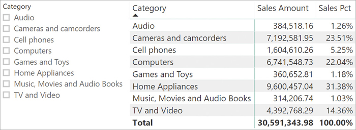
The value of Sales Pct is computed by the following measure:
Sales Pct :=
DIVIDE (
SUMX ( Sales, Sales[Quantity] * Sales[Net Price] ),
SUMX ( ALL ( Sales ), Sales[Quantity] * Sales[Net Price] )
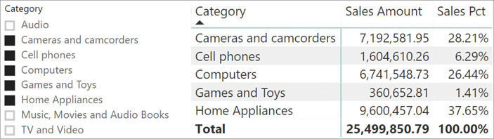
)Because the denominator uses the ALL function, it always computes the grand total of all sales, regardless of any filter. As such, if one uses the slicer to reduce the number of categories shown, the report still computes the percentage against all the sales. For example, Figure 3-18 shows what happens if one selects some categories with the slicer.

Some rows disappeared as expected, but the amounts reported in the remaining rows are unchanged. Moreover, the grand total of the matrix no longer accounts for 100%. If this is not the expected result, meaning that you want the percentage to be computed not against the grand total of sales but rather only on the selected values, then ALLSELECTED becomes useful.
Indeed, by writing the code of Sales Pct using ALLSELECTED instead of ALL, the denominator computes the sales of all categories considering all and only the filters outside of the matrix. In other words, it returns the sales of all categories except Audio, Music, and TV.
Sales Pct :=
DIVIDE (
    SUMX ( Sales, Sales[Quantity] * Sales[Net Price] ),
    SUMX ( ALLSELECTED ( Sales ), Sales[Quantity] * Sales[Net Price] )
)
The result of this latter version is visible in Figure 3-19.
The total is now 100% and the numbers reported reflect the percentage against the visible total, not against the grand total of all sales. ALLSELECTED is a powerful and useful function. Unfortunately, to achieve this purpose, it ends up being an extraordinarily complex function too. Only much later in the book will we be able to explain it in full. Because of its complexity, ALLSELECTED sometimes returns unexpected results. By unexpected we do not mean wrong, but rather, ridiculously hard to understand even for seasoned DAX developers.
When used in simple formulas like the one we have shown here, ALLSELECTED proves to be particularly useful, anyway.
Conclusions
As you have seen in this chapter, basic table functions are already immensely powerful, and they allow you to start creating many useful calculations. FILTER, ALL, VALUES and ALLSELECTED are extremely common functions that appear in many DAX formulas.
Learning how to mix table functions to produce the result you want is particularly important because it will allow you to seamlessly achieve advanced calculations. Moreover, when mixed with the power of CALCULATE and of context transition, table functions produce compact, neat, and powerful calculations. In the next chapters, we introduce evaluation contexts and the CALCULATE function. After having learned CALCULATE, you will probably revisit this chapter to use table functions as parameters of CALCULATE, thus leveraging their full potential.