Gathering information about the data model

The first step for optimizing a data model is gathering information about the cost of the objects in the database. This section describes the tools and the techniques to collect all the data that help in prioritizing the possible optimizations of the physical structure.

Table 18-1 shows the pieces of information to collect from each object in a database.

Table 18-1 Information to collect for each object in a database

In general, object size strongly depends on the number of unique values in the columns being used or referenced. For this reason, the number of unique values in a column, also known as column cardinality, is the single most important piece of information to gather from a database.

In Chapter 17, “The DAX engines,” we introduced the Dynamic Management Views (DMVs) to retrieve information about the objects in the VertiPaq storage engine. The following sections describe how to interpret the relevant information through VertiPaq Analyzer, which simplifies the collection of data from DMVs.

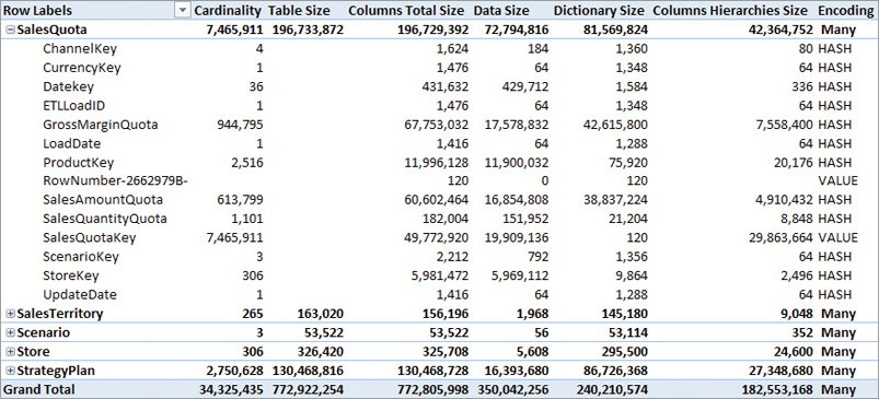
The first piece of information to consider in a data model is the size of each table, in terms of cardinality (number of rows) and size in memory. Figure 18-1 shows the Table section of VertiPaq Analyzer executed on a Contoso data model in Power BI. The model used in this example contains more tables and data than the simplified data model previously used throughout the book.

The Table Size column represents the amount of memory used to store the compressed data in VertiPaq, whereas the Cardinality column shows the number of rows of each table. By drilling down a table name, it is possible to see the details of each column. At the column level, Cardinality shows the number of unique values in the entire table; however, the Table Size value is not available because each column only has the cost shown in Columns Total Size. For example, Figure 18-2 shows the columns available in the largest table of the data model, SalesQuota; note that the total size of each column is extremely variable within the same table.

Each column reported by VertiPaq Analyzer carries a specific meaning described in the following list:

• Cardinality: Object cardinality; the number of rows in a table or the number of unique values in a column, depending on the level of detail in the report.

• Rows: Number of rows in the table. This metric is shown in the columns report (visible later in Figure 18-3) and not in the table report (in Figure 18-2), where the same information is available in the Cardinality metric, at the table detail level of the report.

• Table Size: Size of the table in bytes. This metric contains the sum of Columns Total Size, User Hierarchies Size, and Relationships Size.

• Columns Total Size: Size in bytes of a column. This metric contains the sum of Data Size, Dictionary Size, and Columns Hierarchies Size.

• Data Size: Size in bytes of all the compressed data in segments and partitions. It does not include dictionary and column hierarchies. This number depends on the compression of the column, which, in turn, depends on the number of unique values and the distribution of the data across the table.

• Dictionary Size: Size in bytes of dictionary structures. This number is only relevant for columns with hash encoding; it is a small fixed number for columns with value encoding. The dictionary size depends on the number of unique values in the column and on the average length of the strings in case of a text column.

• Columns Hierarchies Size: Size in bytes of the automatically generated attribute hierarchies for columns. These hierarchies are necessary to access a column in MDX, and they are also used by DAX to optimize filter and sort operations.

• Encoding: Type of encoding (hash or value) used for the column. The encoding of a column is selected automatically by the VertiPaq compression algorithm.

• User Hierarchies Size: Bytes of user-defined hierarchies. This structure is computed at the table level, and its values are only visible at the table level detail in a VertiPaq Analyzer report. The user hierarchy size depends on the number of unique values and on the average length of the strings of the columns used in the hierarchy itself.

• Relationship Size: Bytes of relationships between tables. The relationship size is related to the table on the many-side of a relationship. The size of a relationship depends on the cardinality of the columns involved in the relationship, although this is usually a tiny fraction of the cost of the table.

• Table Size %: Ratio of Columns Total Size versus Table Size.

• Database Size %: Ratio of Table Size versus Database Size, which is the sum of Table Size for all the tables.

• Segments #: Number of segments. All the columns of a table have the same number of segments of the table.

• Partitions #: Number of partitions. All the columns of a table have the same number of partitions of the table.

• Columns #: Number of columns.

The first possible optimization using VertiPaq Analyzer reports is removing any columns that are not useful for the reports and that are expensive in memory. For example, the data shown in Figure 18-2 highlights that one of the most expensive columns of the SalesQuota table is SalesQuotaKey. SalesQuotaKey is not used in any report, and it is not required by the data model structure—as it happens for columns used in relationships. Indeed, the SalesQuotaKey column could be removed from the model without affecting any report and calculation, saving both refresh time and precious memory.

The process of identifying the most expensive columns is made simpler by using another report available in VertiPaq Analyzer shown in Figure 18-3. This Columns report shows all the columns in a flattened list where the reported name is the concatenation of the table and column names, sorting the list by descending Columns Total Size.

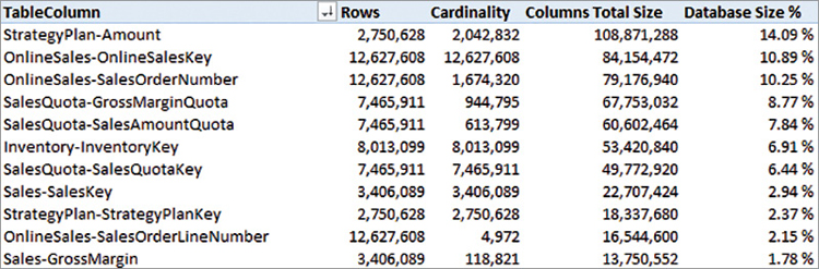
Two of the three most expensive columns of the entire Contoso data model, OnlineSalesKey and SalesOrderNumber in the OnlineSales table, are seldom used in a report at the aggregated level. Each of these two columns imported in VertiPaq requires 10% of the data size of the entire data model. By removing these two columns, it is possible to save 20% of the database size. Being aware of the cost of every column helps one choose what to keep in the data model and what is too expensive relative to its analytical value.

The reason why the report in Figure 18-3 shows Rows and Cardinality side-by-side is to help recognize columns that are unique in a table. When the two numbers are close or identical, it is not useful to create summarized results over a column unless it is the target of an aggregation, such as the Amount column in the StrategyPlan table.

Another important piece of information available in VertiPaq Analyzer is included in the Relationships report shown in Figure 18-4. This report makes it easy to identify expensive relationships present in a data model, even though there are no critical situations in this specific example.

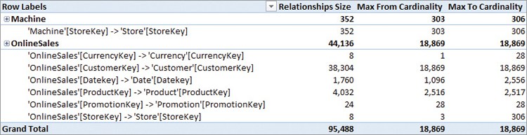
In VertiPaq, relationships with a cardinality larger than 1 million unique values are particularly expensive, impacting the storage engine cost of any request involving that relationship. A common rule of thumb is to start paying attention to a relationship whenever its cardinality exceeds 100,000. Such relationships usually do not produce visible performance issues, but their presence starts to be measurable in hundreds of milliseconds and could create problems with any future growth of the database. While a single large relationship does not necessarily slow down a report visibly, its presence can undermine the performance of more complex calculations and reports.

An awareness of the cardinality of tables and columns is important in any further analyses of a DAX query’s performance. While this information could be retrieved by running simple DAX queries, it is faster and more efficient to use a tool like VertiPaq Analyzer to collect this data automatically—spending more time evaluating the metrics obtained rather than manually running trivial queries on the data model.

Denormalization

The first optimization that can be applied to a data model is to denormalize data. Every relationship has a memory cost and an additional overhead when the engine transfers the filter from one table to another. Purely from a performance point of view, an optimal model would be one made of a single table. However, such an approach would be less than usable and would force a single granularity for all the measures. Thus, an optimal data model is organized as a star schema around each table defined for measures sharing the same granularity. For this reason, one should denormalize unnecessary related tables, thus reducing the number of columns and relationships in the data model.

The denormalization required in a data model for DAX is usually counterintuitive for anyone with some experience in data modeling for a relational database. For instance, consider a simple data model where a Payment table has two columns, Payment Code and Payment Description. In a relational database, a table with Code and Description is commonly used to avoid duplicating the description content in each row of a Transactions table. It is common practice to only store the Payment Code in Transactions to save space in a relational model.

Table 18-2 shows a denormalized version of the Transactions table. There are many rows with duplicated values of Credit Card and Cash in the Payment Type Description column.

Table 18-2 Transactions table with Payment Type denormalized in the Code and Description columns

By using a separate table containing all the payment types, it is possible to only store the Payment Type Code in the Transactions table, as shown in Table 18-3.

Table 18-3 Transactions table normalized, with Payment Type Code only

By storing the description of payment types in a separate table (see Table 18-4), there is only one row for each payment type code and description. That table in a relational database reduces the total amount of space required, by avoiding the duplication of a long string in the Transactions table.

Table 18-4 Payment Type table that normalizes Code and Description

However, this optimization, which works perfectly fine for a relational database, might be a bad choice in a data model for DAX. The VertiPaq engine automatically creates a dictionary for each column, which means that the Transactions table will not pay a cost for duplicated descriptions as would be the case in a relational model.

In terms of space saving, the denormalization is always better by denormalizing a single column in a separate table; on the other hand, the denormalization of many columns in a single table—as is the case for the attributes of a Product—might be more expensive than using a normalized model. For example, we can compare the memory cost between a normalized and a denormalized model:

• Memory cost for normalized model:

  • Column Transactions[Type Code]

  • Column Payments[Type Code]

  • Column Payments[Type Description]

  • Relationship Transactions[Type Code] – Payments[Type Code]

• Memory cost for denormalized model:

  • Column Transactions[Type Code]

  • Column Transactions[Type Description]

The denormalized model removes the cost of the Payments[Type Code] column and the cost of the relationship on Transactions[Type Code]. However, the cost of the Type Description column is different between Transactions and Payments tables, and in a very large table, the difference might be in favor of the normalized model. However, usually the aggregation of a column performs better when a filter is applied to another column of the same table, rather than a filter on a column in another table connected through a relationship. Does this justify a complete denormalization of the data model into a single table? Absolutely not! In terms of usability, the star schema should be always the preferred choice because it is a good trade-off in terms of resource usage and performance.

A star schema contains a table for each business entity such as Customer and Product, and all the attributes related to an entity are completely denormalized in such tables. For example, the Product table should have attributes such as Category, Subcategory, Model, and Color. This model works well whenever the cardinality of the relationship is not too large. As mentioned before, 1 million unique values is the threshold to define a large cardinality for a relationship, although 100,000 unique values already classifies a relationship as a potential risk for the performance of the queries.

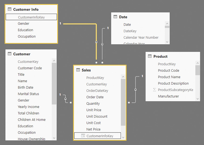
In order to understand why the cardinality of a relationship is important for performance, it is useful to know what happens by applying a filter on a column. Consider the schema in Figure 18-5, where there are relationships between the Sales table and Product, Customer, and Date. By querying the data model filtering customers by gender, the engine transfers the filter from Customer to Sales by specifying the list of customer keys that belong to each gender type included in the query. If there are 10,000 customers, any list generated by a filter cannot be larger than this number. However, if there are 6 million customers, a filter by a single gender type might generate a list of unique keys, resulting in around 3 million unique values for each gender. A large number of keys involved in a relationship always has an impact in performance, even though in absolute terms said impact also depends on the version of the engine and on the hardware being used (CPU clock, cache size, RAM speed).

What can be done to optimize the data model when a relationship involves millions of unique values? If the measured performance degradation is not compatible with the query latency requirements, one might consider other forms of denormalization that reduce the cardinality of the relationship or that remove entirely the need for a relationship in certain queries. In the previous example, one might consider denormalizing the Gender column in the Sales table, in the event it is the only case where they need to optimize performance. If there are more columns to optimize, consider creating another table with the columns of Customer table that users query often and that have a low cardinality (and a low selectivity).

For instance, consider a table called Customer Info with Gender, Occupation, and Education columns. If the cardinality of these columns is 2, 5, and 5 values, respectively, a table with all the possible combinations has 50 rows (2 × 5 × 5). A query on any of these columns will be much faster because the filter applied to Sales will have a very short list of values. In terms of usability, the user will see two groups of attributes for the same entity, corresponding to the two tables, Customer and Customer Info. This is not an ideal situation. For this reason, this optimization should only be considered when strictly necessary, unless the same result can be obtained by using the Aggregations feature in the Tabular model.

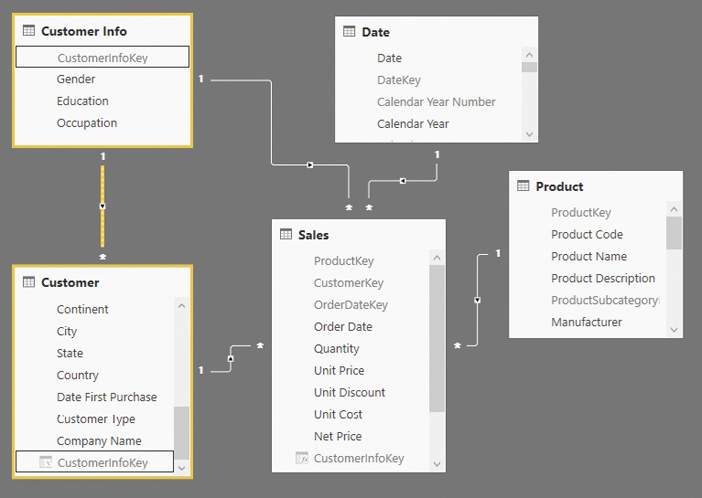
It is important that both tables have a direct relationship with the Sales table, as shown in Figure 18-6.

The CustomerInfoKey column should be added to the Sales table before any data is imported into it so that it is a native column. As discussed in Chapter 17, native columns are better compressed than calculated columns. However, a calculated column could also be created with the following DAX expression:

Click here to view code image

Sales[CustomerInfoKey] =
LOOKUPVALUE (
    'Customer Info'[CustomerInfoKey],
    'Customer Info'[Gender], RELATED ( Customer[Gender] ),
    'Customer Info'[Occupation], RELATED ( Customer[Occupation] ),
    'Customer Info'[Education], RELATED ( Customer[Education] )
)

From a user experience perspective, the columns that are denormalized in the Customer Info table should be hidden from the Customer table. Showing the same attributes (Gender, Occupation, and Education) in two tables would generate confusion. However, by hiding these attributes from the Customer table, it is not possible to create a report with the list of customers with a certain Occupation without looking at the transactions in the Sales table. In order to avoid losing such features, the model should be enhanced including an inactive relationship, which can be activated if needed. We need specific measures to activate that relationship, as we will see later in the optimized Sales Amount measure. Figure 18-7 shows that there is an active relationship between the Customer Info table and the Sales table, and an inactive relationship between the Customer Info table and the Customer table.

The relationship between Customer Info and Customer can be activated whenever there is any other filter active in the Customer table. For example, consider the following definition of the Sales Amount measure:

Click here to view code image

Sales Amount :=
IF (
    ISCROSSFILTERED ( Customer[CustomerKey] ),
    CALCULATE (
        [Sales Internal],
        USERELATIONSHIP ( Customer[CustomerInfoKey], 'Customer Info'[CustomerInfoKey] ),
        CROSSFILTER ( Sales[CustomerInfoKey], 'Customer Info'[CustomerInfoKey], NONE )
    ),
    [Sales Internal]
)

The cross filter is only active in the Customer table when there is a filter on any column of the Customer table, unless the relationship between Sales and Customer is bidirectional. Indeed, when the cross filter is active, the relationship between Customer and Customer Info is enabled by using USERELATIONSHIP, automatically disabling the other relationship between Customer Info and Sales. Furthermore, the CROSSFILTER in the function is not necessary, but it is a good idea to keep it there; it highlights the intention to disable the filter propagation in the relationship between Customer Info and Sales. The idea is that, since the engine must process a list of CustomerKey values in any case, it is better to reduce such a filter by also including the attributes moved into Customer Info. However, when the user filters columns in Customer Info and not in Customer, the default active relationship uses a better relationship made with a lower number of unique values. Unfortunately, in order to optimize the use of the Customer-Sales relationship in a data model, this DAX pattern must be applied to all the measures that might involve Customer Info attributes. This is not necessary using Aggregations in the data model because the pattern is implemented automatically by the engine without requiring any effort in the DAX code.

Another very common scenario where a high cardinality in a relationship should be denormalized is that of a relationship between two large tables. For example, consider the Sales Header and Sales Detail tables in the data model in Figure 18-8.

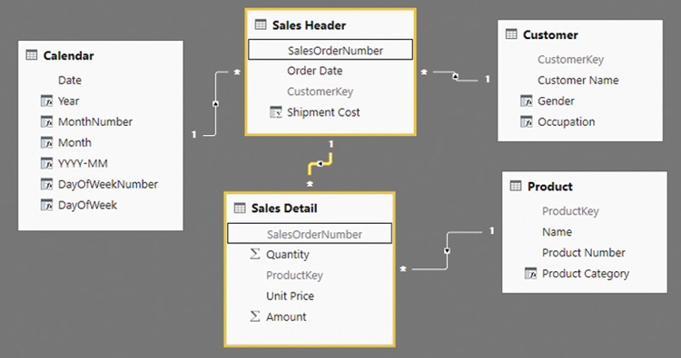
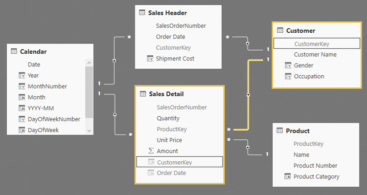
This situation is common because many normalized relational databases are composed of this same design. However, the relationship between Sales Header and Sales Detail is particularly dangerous for a DAX query because of the high number of unique values. Any query grouping the Quantity column (from Sales Detail) by Customer[Gender] transfers a filter from Sales Header to Sales Detail through the SalesOrderNumber column. A better design is possible by denormalizing in Sales Detail all the relationships stored in Sales Header. In practice, there should be two star schemas sharing the same dimensions. The only purpose of the denormalization is to avoid passing a filter through the relationship between Sales Header and Sales Detail, which no longer exists in the new design shown in Figure 18-9.

Use the right degree of denormalization in a data model for DAX, especially for performance reasons. The best practices described in this section provide a good balance between usability and performance.

Columns cardinality

The cardinality of a column is the number of unique values that the column contains. This number is important to reduce the size of the column, which has a direct impact on VertiPaq scan performance. Another reason to reduce the cardinality of a column to a necessary minimum is that many DAX operations, such as iterations and filters, have an execution time that directly depends on this number. Often, the cardinality of a column is more important than the number of rows of the table containing the column.

The data model designer should identify the cardinality of a column and consider possible optimizations if the column is to be used in relationships, filters, or calculations. There are several common scenarios to consider:

• Key of a relationship: The cardinality of the column cannot be changed unless the cardinality of the related table is changed, too. See the “Denormalization” section, earlier in this chapter.

• Numeric value aggregated in a measure: Do not change the precision of a number if that number represents a quantity or the amount of a monetary transaction. However, if a number represents a measure with a floating-point value, one might consider removing the decimals that are not relevant. For example, when collecting temperatures, the value could be rounded down to the closest decimal digit; the removed part is probably lower than the precision of the measuring tool.

• Low cardinality text description: The only impact is on dictionary size in case the column has many unique values. There are no advantages in moving the column into a separate table because the dictionary would be the same. Keep this column if users need it.

• High cardinality text notes: Potentially different for every row of the table, but it is not a big issue if most of the rows have a blank value.

• Pictures: This column is required to display graphics in a client tool—for example, a picture of a product. This data type is not available in Power BI; storing the URL of an image that is loaded dynamically is a better alternative that saves memory.

• Transaction ID: This column has a high cardinality in a large table. Consider removing it if it is not necessary in DAX queries. If used in drill-through operations—for example, to see the transactions that form a particular aggregation—consider splitting the number/string into two or more parts, each with a smaller number of unique values.

• Date and time: Consider splitting the column into two parts. More on this in the following section in this chapter, “Handling date and time.”

• Audit columns: A table in a relational database often has standard columns used for auditing purposes—for instance, timestamp and user of last update. These columns should not be imported in a model stored by VertiPaq, unless required for drill-through. In that case, consider splitting the timestamp following the same rules applied to date and time.

As a rule of thumb, consider that reducing the cardinality of a column saves memory and improves performance. Because reducing cardinality might imply losing information and/or accuracy, be careful in considering the implications of these optimizations.

Handling date and time

Almost any data model has one or more date columns. Every so often, the time is also an interesting dimension of analysis. Usually, these columns come from original Datetime columns in the data source. There are several best practices to optimize these types of columns.

First and foremost, date and time should be always split into two separate columns, without using calculated columns to do so. The split should take place by reading the original column in two different columns of the data model: one for the date, the other for the time. For example, reading a TransactionExecution column from a table in SQL Server, one should use the following syntax in a T-SQL query to create two columns, TransactionDate and TransactionTime:

Click here to view code image

 ...
CAST ( TransactionExecution AS DATE ) AS TransactionDate,
CAST ( TransactionExecution AS TIME ) AS TransactionTime,
...

It is very important to do this split operation; otherwise, the model would have a column in which dictionary and cardinality would increase every day. Moreover, analyzing a timestamp in Tabular is very hard. A Date table needs an exact match with the date, and the Datetime column would not work correctly in a relationship with the Date column of a Date table.

A Date column usually has a good granularity: 10 years correspond to less than 3,700 unique values, and even 100 years still fall within a manageable order of magnitude. Moreover, time intelligence functions require a complete calendar for each year considered, so removing days (for example, keeping only one day per month) is not an optimization to consider.

The Time column, on the other hand, should be subject to more considerations. With a Time column, one should consider creating a Time table, which contains one row for each point in the chosen granularity. The time should be rounded to the same granularity as the one chosen for the Time table. The Time table will make it easy to consider different time periods: for example, morning and evening, or 15-minute intervals. Depending on the data and the analysis required, the time could be rounded down to the closest hour or millisecond—even though the latter is very unlikely. Table 18-5 shows the different cardinality corresponding to different precision levels.

Table 18-5 Cardinality corresponding to different precision levels for a Time column

Choosing the millisecond precision is usually the worst choice, and a precision down to the second still has a relatively high number of unique values. Most of the times the precision choice will be in a range between hours and minutes. At this point, one might think that the minute precision is a safe choice because it has a relatively low cardinality. However, remember that the compression of a column depends on the presence of duplicated values in contiguous rows. Thus, moving from a minute to 15-minute precision can have a big impact on the compression of large tables.

The choice between rounding to the closest second/minute or truncating the detail not needed for the analysis depends on analytical requirements. Here is an example of the T-SQL code that truncates a time to different precision levels:

Click here to view code image

-- Truncate to the second
DATEADD (
    MILLISECOND,
    - DATEPART ( MILLISECOND, CAST ( TransactionExecution AS TIME(3) ) ),
    CAST ( TransactionExecution AS TIME(3) )
)
-- Truncate to the minute
DATEADD (
    SECOND,
    - DATEPART (SECOND, CAST ( TransactionExecution AS TIME(0) ) ),
    CAST ( TransactionExecution AS TIME(0) )
)

-- Truncate to 5 minutes
--   change 5 to 15 to truncate to 15 minutes
--   change 5 to 60 to truncate to the hour
CAST (
    DATEADD (
        MINUTE,
        ( DATEDIFF (
              MINUTE,
              0,
              DATEADD (
                  SECOND,
                  - DATEPART ( SECOND, CAST ( TransactionExecution AS TIME(0) ) ),
                  CAST ( TransactionExecution AS TIME(0) )
              )
          ) / 5 ) * 5,
        0
    ) AS TIME(0)
)

The following T-SQL code shows examples for rounding time instead of truncating it:

Click here to view code image

-- Round to the second
CAST ( TransactionExecution AS TIME(0) )

-- Round to the minute
CAST ( DATEADD (
    MINUTE,
    DATEDIFF (
        MINUTE,
        0,
        DATEADD ( SECOND, 30, CAST ( TransactionExecution AS TIME(0) ) )
    ),
    0
) AS TIME ( 0 ) )

-- Round to 5 minutes
--   change 5 to 15 to truncate to 15 minutes
--   change 5 to 60 to truncate to the hour
CAST ( DATEADD (
    MINUTE,
    ( DATEDIFF (
        MINUTE,
        0,
        DATEADD ( SECOND, 5 * 30, CAST ( TransactionExecution AS TIME(0) ) )
      ) / 5 ) * 5,
    0
) AS TIME ( 0 ) )

Similar transformations can be applied in Power Query when importing data, though for tables with millions of rows a transformation made in the original data source may provide better performance.

When storing millions of new rows every day in a single table, these details can make a big difference in memory usage and performance. At the same time, do not spend too much time optimizing a data model that does not require very high a level of compression; after all, reducing the precision means removing some information that will no longer be available for deeper insights if needed.

Calculated columns

A calculated column stores the result of a DAX expression evaluated row-by-row during a table refresh. For this reason, calculated columns might be considered as a possible way to optimize query execution time. However, a calculated column has hidden costs, and it is only a good optimization technique under specific conditions.

Calculated columns should be considered as viable options only in these two situations:

• Group or filter data: If a calculated column returns a value used to group or filter data, there is no alternative other than creating the same value before importing data into the data model. For example, the price of a product might be classified into Low, Medium, and High categories. This value is usually a string, especially when the user makes it available as a selection.

• Precalculate complex formulas: A calculated column can store the result of a complex calculation that is not sensitive to filters made at query time. However, it is very hard to establish when this produces a real computational advantage, and it is necessary to measure the presence of a real advantage at query time in order to justify its use.

Do not make the wrong assumption that any calculated column is faster than doing the same computation at query time. This is often inaccurate. Other times, the advantage is barely measurable and does not balance out the cost of the calculated column. There should be a relevant performance improvement at query time to justify a calculated column for optimization reasons. There are also many factors to consider when evaluating the cost/benefit ratio of a calculated column against an equivalent calculation made at runtime in a measure.

A calculated column is not as optimized as a native column. It might have a lower compression rate compared to native columns of the table because it does not take part in the heuristic that VertiPaq executes to find the optimal sort order of the data in each segment. Only a column storing a very low number of unique values might benefit from a good compression, but this is usually the result of logical conditions and not of numeric expressions.

For example, consider the case of a simple calculated column:

Click here to view code image

Sales[Amount] = Sales[Quantity] * Sales[Price]

If there are 100 unique values in Quantity and 1,000 unique values in Price, the resulting Amount column might have a cardinality between 1 and 100,000 unique values, depending on the actual values in the columns and on their distribution across table rows. Usually, the larger the number of rows in the table, the higher the number of unique values found in the Amount column—because of statistical distribution. With a dictionary that is one or two orders of magnitude larger than the original columns, the compression is usually worse. What about query performance? It depends, and it should be measured case-by-case in order to get a correct answer, considering the two possible calculations: one based on a calculated column and the other completely dynamic and based on measures.

A simple measure can sum the Amount calculated column:

Click here to view code image

TotalAmountCC := SUM ( Sales[Amount] )

The alternative dynamic implementation transfers the expressions of the calculated column in an iterator over the table:

Click here to view code image

TotalAmountM := SUMX ( Sales, Sales[Quantity] * Sales[Price] )

Is the cost of scanning the single Sales[Amount] column smaller than scanning the two original Sales[Quantity] and Sales[Price] columns? It is impossible to estimate this in advance, so it must be measured. Usually, the difference between these two options is only visible in very large tables. In small tables the performance might be very close, so the calculated column is not worth its memory footprint.

Most of the time, calculated columns used to compute aggregated values can be replaced by using the same expressions in iterators such as SUMX and AVERAGEX. In the previous example, TotalAmountM is a measure that dynamically executes the same expression defined in the calculated Amount column, used by the simple aggregation in TotalAmountCC.

A different evaluation is necessary when a context transition is present in an iterator. For example, consider the following DAX measure in a model where the Sales Header and Sales Detail tables are connected through a relationship:

Click here to view code image

AverageOrder :=
AVERAGEX (
    'Sales Header',
    CALCULATE (
        SUMX (
            'Sales Detail',
            'Sales Detail'[Quantity] * 'Sales Detail'[Unit Price]
        ),
        ALLEXCEPT ( 'Sales Detail', 'Sales Header' )
    )
)

In this case, the context transition within the loop can be very expensive, especially if the Sales Header table contains millions of rows or more. Storing the value in a calculated column will probably save a lot of execution time.

Click here to view code image

'Sales Header'[Amount] =
CALCULATE (
    SUMX (
        'Sales Detail',
        'Sales Detail'[Quantity] * 'Sales Detail'[Unit Price]
    )
)

AverageOrder :=
AVERAGEX (
    'Sales Header',
    'Sales Header'[Amount]
)

We will never grow tired of repeating that these examples are guidelines. One should measure the performance improvements of a calculated column and its related memory cost in order to decide whether to use it or not.

Consider that a calculated column can be avoided by creating the same value for a native column in the data source when populating the table—for example, using an SQL statement or a Power Query transformation. A useful calculated column should leverage the VertiPaq engine, providing a faster and more flexible way to compute a column than reading the entire table again from the data source. Usually, this happens when the calculated column expression aggregates rows from tables other than the one it belongs to; the previous Amount calculated column in the Sales Header table is an example of such condition.

Finally, a calculated column increases the time to refresh a data model especially because it is an operation that cannot scale on multiple threads, as explained in more detail in a following section, “Processing of calculated columns.”

At this point, it should be clear that calculated columns are expensive for two reasons:

• Memory: The values are persisted using a nonoptimal compression.

• Duration of Refresh: The process of calculated columns is a sequential operation using a single thread, which results in a nonscalable operation also in large servers.

With that said, calculated columns prove useful in many scenarios. We do not want to pass on the message that calculated columns are always to be avoided. Instead, be aware of their cost and make an educated decision on whether to use them or not. In the next section we describe a good example where calculated columns really shine in improving performance.

ExpensiveTransactions :=
COUNTROWS (
    FILTER (
        Sales,
        VAR UnitPrice =
            IF (
                Sales[Unit Discount] > 0,
                RELATED ( 'Product'[Unit Price] ),
                Sales[Net Price]
            )
        VAR IsLargeTransaction = UnitPrice * Sales[Quantity] > 100
        VAR IsLargePrice = UnitPrice > 70
        VAR IsExpensive = IsLargeTransaction || IsLargePrice
        RETURN
            IsExpensive
    )
)

Sales[IsExpensive] =
VAR UnitPrice =
    IF (
        Sales[Unit Discount] > 0,
        RELATED ( 'Product'[Unit Price] ),
        Sales[Net Price]
    )
VAR IsLargeTransaction = UnitPrice * Sales[Quantity] > 100
VAR IsLargePrice = UnitPrice > 70
VAR IsExpensive = IsLargeTransaction || IsLargePrice
RETURN
    IsExpensive

ExpensiveTransactions :=
CALCULATE (
    COUNTROWS ( Sales ),
    Sales[IsExpensive] = TRUE
)

Choosing the right columns to store

The previous section about calculated columns explained that storing a column that can be computed row-by-row using other columns of the same table is not always an advantage. The same consideration is also valid for native columns of the table. When choosing the columns to store in a table, consider the memory size and the query performance. Good optimizations of resource allocation (and memory in particular) are possible by doing the right evaluation in this area.

We consider the following types of columns in a table:

• Primary or alternate keys: The column contains a unique value for each row of the table.

• Qualitative attributes: The column can be text or number, used to group and/or filter rows in a table; for instance, name, color, city, country.

• Quantitative attributes: The number is a value used both as a filter (for example, less than a certain value) and as an argument in a calculation, such as price, amount, quantity.

• Descriptive attributes: The column contains text providing additional information about a row, but its content is never used to filter or to aggregate rows—for example, notes, comments.

• Technical attributes: Information recorded in the database for technical reasons, without a business value, such as username of last update, timestamp, GUID for replication.

The general principle is to try to minimize the cardinality of the columns imported into a table, not importing columns that have a high cardinality and that are not relevant for the analysis. However, every type of column deserves additional considerations.

The columns for primary or alternate keys are necessary if there are one or more one-to-many relationships with other tables. For instance, the product code and the product key columns of a table of products are certainly required columns. However, a table should not include a primary or alternate key column not used in a relationship with other tables. For example, the Sales table might have a unique identifier for each row in the original table. Such a column has a cardinality that corresponds to the number of rows of the Sales table. Moreover, a unique identifier is not necessary for relationships because no tables target Sales for a relationship. For these reasons, it is a very expensive column in terms of memory, and it should not be imported in memory. In a composite data model, a similar high-granularity column could be accessed only through DirectQuery without being stored in memory, as described later in the “Optimizing column storage” section of this chapter.

A table should always include qualitative attributes that have a low cardinality because they have a good compression and might be useful for the analysis. For example, the product category is a column that has a low cardinality, related to the Product table. In case there is a high cardinality, we should consider carefully whether to import the column or not because its storage memory cost can be high. The high selectivity might justify the cost, but we should check that filters in queries usually select a low number of values in that column. For instance, the production lot number might be a piece of information included in the Sales table that users want to filter at query time. Its high cost might be justified by a business need to apply this filter in certain queries.

All the quantitative attributes are generally imported to guarantee any calculation, although we might consider skipping columns providing redundant information. Consider the Quantity, Price, and Amount columns of a Sales table, where the Amount column contains the result of the product between Quantity and Price. We probably want to create measures that aggregate each of these columns; yet we will probably calculate the price as a weighted average considering the sum of amount and quantity, instead of a simple average of the price considering each transaction at the same level. This is an example of the measure we want to define:

Click here to view code image

Sum of Quantity := SUM ( Sales[Quantity] )

Sum of Amount   := SUM ( Sales[Amount] )

Average Price   := DIVIDE ( [Sum of Amount], [Sum of Quantity] )

By looking at these measures, we might say that we only need to import Quantity and Amount in the data model, without importing the Price column, which is not used by these measures. However, if we consider the cardinality of the columns, we start to have doubts. If there are 100 unique values in the Quantity column, and there are 10,000 unique values in the Price column, we might have up to 1,000,000 unique values in the Amount column. At this point, we might consider importing only the Quantity and Price columns, using the following definition of the measures in the data model; only Sum of Amount changes, the other two measures did not change:

Click here to view code image

Sum of Quantity := SUM ( Sales[Quantity] )

Sum of Amount   := SUMX ( Sales, Sales[Quantity] * Sales[Price] )

Average Price   := DIVIDE ( [Sum of Amount], [Sum of Quantity] )

The new definition of the Sum of Amount measure might be slower because it has to scan two columns instead of one. However, these columns might be smaller than the original Amount. Trying to predict the faster option is very hard because we should also consider the distribution of the values in the table, and not only the cardinality of the column. We suggest measuring the memory used and the performance in both scenarios before making a final decision. Based on our experience, removing the Amount column in a small data model can be more important for Power BI and Power Pivot. Indeed, the available memory in personal computers is usually more limited than that of a server, and a smaller memory footprint also produces a faster loading time opening the smaller file. At any rate, in a large table with billions of rows stored in an Analysis Services Tabular model, the performance penalty of the multiplication between two columns (Quantity and Price) could be larger than the increased memory scan time for the Amount column. In this case, the better response time for the queries justifies the higher memory cost to store the Amount column. Regardless, we should measure size and performance in each specific case because the distribution of data plays a key role in compression and affects any decision pertaining to it.

We should consider whether to import descriptive attributes or not. In general, they have a high storage cost for the dictionary of the column when imported in memory. A few examples of descriptive attributes are the Notes field in an invoice and the Description column in the Product table. Usually, these attributes are mainly used to provide additional information about a specific entity. Users hardly use this type of column to group or filter data; the typical use case is to get detailed drill-through information. The only issue with including these columns in the data model is their memory storage cost, mainly related to the column dictionary. If the column has many blank values and a low number of unique nonblank values in the table, then its dictionary will be small and the column cost will be more acceptable. Nevertheless, a column containing the transcription of conversations made in a call center is probably too expensive for a Service Calls table containing date, time, duration, and operator who managed the call. When the cost of storing descriptive attributes in memory is too expensive, we can consider only accessing them through DirectQuery in a composite data model.

A particular type of descriptive attribute is the information provided as detail for transactions in a drill-through operation. For example, the invoice number or the order number of a transaction is an attribute that has a high cardinality, but that could be important for some reports. In this case, we should consider the particular optimizations for drill-through attributes described in the next section, “Optimizing column storage.”

Most of the time, there is no reason to import columns for technical attributes, such as timestamp, date, time, and operator of the last update. This information is mainly for auditing and forensic requirements. Unless we have a data model specifically built for auditing requirements, the need for this information is usually low in an analytical solution. However, technical attributes are good candidates for columns accessed only through DirectQuery in a composite data model.

Optimizing column storage

The best optimization for a column is to remove the column from a table entirely. In the previous section, we described when this decision makes sense based on the type of columns in a table. Once we define the set of columns that are part of the data model, we can still use optimization techniques in order to reduce the amount of memory used, even though each optimization comes with side effects. In case the composite data model feature is available, an additional option is that of keeping a column in the data source, only making it accessible through DirectQuery.

SELECT
    LEFT ( TransactionID, 5 ) AS TransactionID_High,
    SUBSTRING ( TransactionID, 6, LEN ( TransactionID ) - 5 ) AS TransactionID_Low,
    ...

SELECT
    TransactionID / 10000 AS TransactionID_High,
    TransactionID % 10000 AS TransactionID_Low,
    ...

SELECT
    FLOOR ( UnitPrice ) AS UnitPrice_Integer,
    UnitPrice - FLOOR ( UnitPrice ) AS UnitPrice_Decimal,
    ...

Sum of Amount :=
SUMX (
    Sales,
    Sales[Quantity] * ( Sales[UnitPrice_Integer] + Sales[UnitPrice_Decimal] )
)

Managing VertiPaq Aggregations

The VertiPaq storage engine can be used for managing aggregations over DirectQuery data sources—and in the future, also over large VertiPaq tables. Aggregations were initially introduced in late 2018 as a Power BI feature. That same feature could later be adopted by other products. The purpose of Aggregations is to reduce the cost of a storage engine request, removing the need for an expensive DirectQuery request in case the data is available in a smaller table containing aggregated data.

The Aggregations feature is not necessarily related to VertiPaq: it is possible to define aggregations in a DirectQuery model so that different tables are queried on the data source, depending on the granularity of a client request. However, the typical use case for Aggregations is defining them in a composite data model, where each table has three possible storage modes:

• Import: The table is stored in memory and managed by the VertiPaq storage engine.

• DirectQuery: The data is kept in the data source; at runtime, every DAX query might generate one or more requests to the data source, typically sending SQL queries.

• Dual: The table is stored in memory by VertiPaq and can also be used in DirectQuery, typically joining other tables stored in DirectQuery or Dual mode.

The principle of aggregations is to provide different options to solve a storage engine request. For example, a Sales table can store the details of each transaction, such as product, customer, and date. When one creates an aggregation by product and month, the aggregated table has a much smaller number of rows. The Sales table could also have more than one aggregation, each one with a precedence used in case of multiple aggregations compatible with the same request. Consider a case where the following aggregations are available in a model with Sales, Product, Date, and Store:

• Product and Date—precedence 50

• Store and Date—precedence 20

If a query required the total of sales by product brand and year, it would use the first aggregation. The same aggregation would be used when drilling down at the month or day level. Indeed, the aggregation that has the Sales data at the Product and Date granularity can solve any query that groups rows by using attributes included in these tables. With the same logic, a query aggregating data by store country and year will use the second aggregation created at the granularity of Store and Date. However, a query aggregating data by store country and product brand cannot use any existing aggregation. Such queries must use the Sales table that has all the details because none of the aggregations available have a granularity compatible with the request. If two or more aggregations are compatible with the request, the choice is made based on the precedence setting defined for each aggregation: The engine chooses the aggregation with the highest precedence. Table 18-6 recaps the aggregations used based on the query request in the examples described.

Table 18-6 Examples of aggregation used, based on query request

The engine chooses the aggregation to use only considering the precedence order, regardless of the aggregation storage mode. Indeed, every aggregation has an underlying table that can be stored either in VertiPaq or in DirectQuery. Common sense would suggest that a VertiPaq aggregation should be preferred over a DirectQuery aggregation. Nevertheless, the DAX engine only follows precedence rules. If a DirectQuery aggregation has a higher precedence over a VertiPaq aggregation, and both are candidates to speed up a request, the engine chooses the DirectQuery aggregation. It is up to the developer to define a good set of precedence rules.

An aggregation can match a storage engine request depending on several conditions:

• Granularity of the relationships involved in the storage engine request.

• Matching of columns defined as GroupBy in the summarization type of the aggregation.

• Summarization corresponding to a simple aggregation of a single column.

• Presence of a Count summarization of the detail table.

These conditions might have an impact on the data model design. A model that imports all the tables in VertiPaq usually is designed to minimize the memory requirements. As described in the previous section, “Choosing the right columns to store,” storing the Quantity and Price columns allows the developer to compute the Amount at query time using a measure such as:

Click here to view code image

Sales Amount := SUMX ( Sales, Sales[Quantity] * Sales[Price] )

This version of the Sales Amount measure might not use an aggregation with a Sum summarization type because the Sum summarization only references a single column. However, an aggregation could match the request if Sales[Quantity] and Sales[Price] have the GroupBy summarization and if there is a Count summarization of the Sales table. For complex expressions it could be hard to define an efficient aggregation, and this could impact the model and aggregation design.

Consider the following code as an educational example. If there are two Sum aggregations for the Sales[Amount] and Sales[Cost] columns, then a Margin measure should be implemented using the difference between two aggregations (Margin1 and Margin2), instead of aggregating the difference computed row-by-row (Margin3).

Click here to view code image

Sales Amount := SUM ( Sales[Amount] )                         -- Can use Sum aggregations
Total Cost   := SUM ( Sales[Cost] )                           -- Can use Sum aggregations
Margin1      := [Sales Amount] - [Total Cost]                 -- Can use Sum aggregations
Margin2      := SUM ( Sales[Amount] ) - SUM ( Sales[Cost] )   -- Can use Sum aggregations

Margin3 := SUMX ( Sales, Sales[Amount] - Sales[Cost] )   -- CANNOT use Sum aggregations

However, the Margin3 measure could match an aggregation that defines the GroupBy summarization for the Sales[Amount] and Sales[Cost] columns and that also includes a Count summarization of the Sales table. Such aggregation would potentially also be useful for the previous definitions of the Sales Amount and Total Cost measures, even though it would be less efficient than a Sum aggregation on the specific column.

As of April 2019, the Aggregations feature is available for DirectQuery tables. While it is not possible to define aggregations for a table imported in memory, that feature might be implemented in the near future. At that point, all these combinations will become possible:

• DirectQuery aggregation over a DirectQuery table

• VertiPaq aggregation over a DirectQuery table

• VertiPaq aggregation over a VertiPaq table (not available as of April 2019)

The ability to create a VertiPaq aggregation over VertiPaq tables will provide a tool to optimize two scenarios for models imported in memory: very large tables (billions of rows) and relationships with a high cardinality (millions of unique values). These two scenarios can be managed by manually modifying the data model and the DAX code as described in the “Denormalization” section earlier in this chapter. The aggregations over VertiPaq tables will automate this process, resulting in better performance, reduced maintenance, and decreased development costs.

Conclusions

In this chapter we focused on how to optimize a data model imported in memory using the VertiPaq storage engine. The goal is to reduce the memory required for a data model, obtaining as a side effect an improvement in query performance. VertiPaq can also be used to store aggregations in composite models, combining the use of the DirectQuery and VertiPaq storage engines in a single model.

The main takeaways of this chapter are:

• Only import in memory the columns required for the analysis.

• Control columns cardinality, as a low cardinality column has better compression.

• Manage date and time in separate tables and store them at the proper granularity level for the analysis. Storing a precision higher than required (e.g., milliseconds) consumes memory and lowers query performance.

• Consider using VertiPaq to store in-memory aggregations for DirectQuery data sources in composite models.