Chapter 2. Time Travel with Delta Lake
Introduction
Data engineering pipelines often go awry, especially when ingesting “dirty” data from external systems. However, in a traditional data lake design, it is hard to undo updates that added objects into a table. In addition, it is challenging to audit data changes which are critical, both in terms of data compliance as well as simple debugging, to understand how data has changed over time. Other data workloads, such as machine learning training, require faithfully reproducing an old version of the data (e.g., to compare a new and old training algorithm on the same data). For example, if some upstream pipeline modifies the source data, data scientists are often caught unaware by such upstream data changes and hence struggle to reproduce their experiments.
All of these issues created significant challenges for data engineers and data scientists before Delta Lake, requiring them to design complex remediations to data pipeline errors or to haphazardly duplicate datasets. Through this chapter, we will explore the capabilities of Delta Lakes that allow data practitioners to go back in time and solve for these challenges. It is uncertain if time travel to the past is physically possible but data practitioners can time travel programmatically with Delta Lake. Delta Lake allows automatic versioning of all data stored in the data lake and we can time travel to any version. It also allows us to create a copy of an existing Delta table at a specific version using the clone command to help with a few time travel use cases. To understand these functionalities and how time travel works, we first need to unpack the file structure of Delta tables and deep dive into each of the components.
Under the hood of a Delta Table
In chapter 2, one of our sections was to focus on unpacking the transaction log. But recall that the transaction log is just one part of the Delta table. In this section, we will focus on the components that make up the Delta table.
The Delta Directory
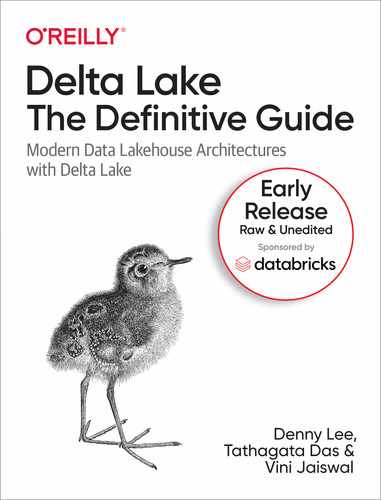
A Delta table is stored within a directory and is composed of the file types shown in Figure 2-1.
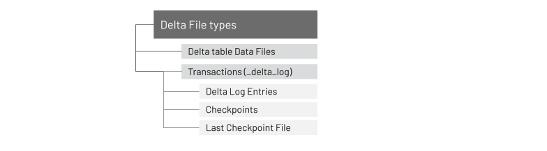
Figure 2-1. Delta Directory structure
As an example, we have a delta table named customer_data located in the filePath: dbfs:/user/hive/warehouse/deltaguide.db
To visualize the delta file system, see below a snippet from our example. You can also follow along with us by using the notebooks present here.
Root of the Delta directory : This is the hive warehouse location where we created a delta table and using the command below, we can explore the contents within the delta directory. For the full output, please refer to this location.
%fs ls dbfs:/user/hive/warehouse/deltaguide.db/customer_data
| path | name | size |
| dbfs:/dbfs:/..filePath../customer_data/_delta_log/ | _delta_log/ | 0 |
| dbfs:/dbfs:/..filePath../customer_data/part-00000-41…-c001.snappy.parquet | part-00000-41...-c001.snappy.parquet | 542929260 |
| dbfs:/dbfs:/..filePath../customer_data/part-00000-45...-c002.snappy.parquet | part-00000-45...-c002.snappy.parquet | 461126371 |
| dbfs:/dbfs:/..filePath../customer_data/part-00000-62...-c000.snappy.parquet | part-00000-62...-c000.snappy.parquet | 540468009 |
| dbfs:/dbfs:/..filePath../customer_data/part-00001-40...-c002.snappy.parquet | part-00001-40...-c002.snappy.parquet | 541858629 |
| dbfs:/dbfs:/..filePath../customer_data/part-00001-a7...-c001.snappy.parquet | part-00001-a7...-c001.snappy.parquet | 542859315 |
| dbfs:/dbfs:/..filePath../customer_data/part-00001-c3...-c000.snappy.parquet | part-00001-c3...-c000.snappy.parquet | 541186721 |
Delta Logs Directory
When a user creates a Delta Lake table, that table’s transaction log is automatically created in the _delta_log subdirectory. As he or she makes changes to that table, those changes are recorded as ordered, atomic commits in the transaction log. Each commit is written out as a JSON file, starting with 000000.json. Additional changes to the table generate subsequent JSON files in ascending numerical order so that the next commit is written out as 000001.json, the following as 000002.json, and so on.
Figure 2-2 shows the logical diagram of Delta Transaction Log Protocol.
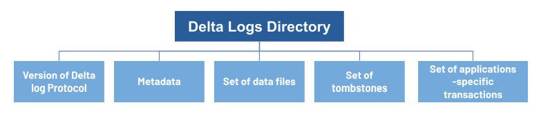
Figure 2-2. Delta Transaction Log Protocol
The state of a table at a given version is called a snapshot and includes the following properties:
-
Version of the Delta log protocol : This is required to correctly read or write the table
-
Metadata of the table (e.g., the schema, a unique identifier, partition columns, and other configuration properties)
-
Set of files present in the table, along with metadata about those files
-
Set of tombstones for files that were recently deleted
-
Set of applications-specific transactions that have been successfully committed to the table
We will explore each of the properties in the upcoming sections and to provide you a mental mapping of how this actually looks from a file system perspective, here is a snippet.
%fs ls dbfs:/fil
ePath/customer_t2/_delta_log
| path | name | size |
| dbfs:/.../customer_t2/_delta_log/.s3-optimization-0 | .s3-optimization-0 | 0 |
| dbfs:/.../customer_t2/_delta_log/.s3-optimization-1 | .s3-optimization-1 | 0 |
| dbfs:/.../customer_t2/_delta_log/.s3-optimization-2 | .s3-optimization-2 | 0 |
| dbfs:/.../customer_t2/_delta_log/00000000000000000010.checkpoint.parquet | 00000000000000000010.checkpoint.parquet | 120950 |
| : : : |
: : : |
: : : |
| dbfs:/.../customer_t2/_delta_log/00000000000000000020.checkpoint.parquet | 00000000000000000020.checkpoint.parquet | 94341 |
| dbfs:/.../customer_t2/_delta_log/00000000000000000020.crc | 00000000000000000020.crc | 97 |
| dbfs:/.../customer_t2/_delta_log/00000000000000000020.json | 00000000000000000020.json | 347291 |
| dbfs:/.../customer_t2/_delta_log/00000000000000000021.crc | 00000000000000000021.crc | 95 |
| dbfs:/.../customer_t2/_delta_log/00000000000000000021.json | 00000000000000000021.json | 41461 |
| dbfs:/.../customer_t2/_delta_log/_last_checkpoint | _last_checkpoint | 26 |
As previously noted, Delta Lake is an open-source storage layer that runs on top of your existing data lake and is fully compatible with Apache Spark APIs. Delta Lake uses versioned Parquet files to store data in your cloud storage, enabling Delta Lake to leverage the efficient compression and encoding schemes that are native to Parquet. Apart from the versions, Delta Lake also stores a transaction log to keep track of all the commits made to the table or blob store directory to provide ACID transactions.
You can use your favorite Apache Spark APIs to read and write data with Delta Lake. As noted in the previous chapter, to create a Delta table, write a DataFrame out in the delta format.
%python# Generate Spark DataFramedata=spark.range(0,5)# Write the table in parquet formatdata.write.format("parquet").save("/table_pq")# Write the table in delta formatdata.write.format("delta").save("/table_delta")
%scala// Generate Spark DataFramevaldata=spark.range(0,5)// Write the table in parquet formatdata.write.format("parquet").save("/table_pq")// Write the table in delta formatdata.write.format("delta").save("/table_delta")
Once you write the files in delta, you will notice that a number of files are created under a folder in the format recognized by Spark as a Parquet table and/or stored in a metastore (e.g. Hive, Glue, etc.).
Note
Note, the files of a metastore-defined table are stored under the default hive/warehouse location though you have an option to specify a location of your choice at the time of writing delta files as noted in the previous example.
To review the underlying file structure, run the following command from your
-table>
The following is the shell command for the parquet table previously generated.
%sh ls -R /dbfs/table_pq//dbfs/table_pq/:part-00000-775edc03-7c05-4190-a964-fcdfc0428014-c000.snappy.parquetpart-00001-94940738-a4e6-4b4b-b30f-797a76b32087-c000.snappy.parquetpart-00003-0e5d49e6-4dd0-4746-8944-f64cba9df97c-c000.snappy.parquetpart-00004-bed772f9-1045-4e3a-8048-e179096e3c25-c000.snappy.parquetpart-00006-e28f9fa4-516b-4cf6-acdd-22d70e8841f2-c000.snappy.parquetpart-00007-5276d994-b9ca-4da8-b594-4bbfafbd7dcb-c000.snappy.parquet
The following is the shell command for the Delta table previously generated.
%sh ls -R /dbfs/table_delta//dbfs/table_delta/:_delta_logpart-00000-775edc03-7c05-4190-a964-fcdfc0428014-c000.snappy.parquetpart-00001-94940738-a4e6-4b4b-b30f-797a76b32087-c000.snappy.parquetpart-00003-0e5d49e6-4dd0-4746-8944-f64cba9df97c-c000.snappy.parquetpart-00004-bed772f9-1045-4e3a-8048-e179096e3c25-c000.snappy.parquetpart-00006-e28f9fa4-516b-4cf6-acdd-22d70e8841f2-c000.snappy.parquetpart-00007-5276d994-b9ca-4da8-b594-4bbfafbd7dcb-c000.snappy.parquet/dbfs/table_delta/_delta_log:00000000000000000000.crc00000000000000000000.json
Majority of Data Practitioners are familiar with Parquet and its structure, let’s simplify the understanding of Delta by comparing it to Parquet.
What is the difference between the Parquet and Delta tables?
The only difference between the Parquet and Delta tables is the _delta_log folder which is the Delta transaction log (more on this in Chapter 2).
What is the same between the Parquet and Delta tables?
In both Parquet and Delta tables, the data itself is in the form of snappy compressed Parquet part files, which is the common format of Spark tables.
-
Apache Parquet is a columnar storage format that is optimized for BI-type queries (group by, aggregates, joins, etc.). Because of this, it is the default storage format for Apache Spark when it writes its data files to storage.
-
Snappy compression was developed by Google to provide high compression/decompression speeds with reasonable compression. By default, Spark tables are snappy compressed Parquet files.
-
By default, the reference implementation of Delta lake stores data files in directories named after partition values for data in that file (i.e.
part1=value1/part2=value2/...) that is why we see part files and a suffix in the name as a globally unique identifier to ensure uniqueness of each file. This is especially important because each directory in cloud object stores are not actual folders but logical representations of folders. For more information on the implications, read more at How to list and delete files faster in Databricks.
The files of a Delta table
ny time data is modified in a Delta table, new files are created as a Version which is a snapshot of the delta table at that specific time and is a result of a set of actions that were performed by the user.
Version 0: Table creation
Let’s start by looking at the Delta table created in the previous section by running the following commands to review the path column of the add metadata.
%python# Read first transactionj0=spark.read.json("/table_delta/_delta_log/00000000000000000000.json")# Review Add Informationj0.select("add.path").where("add is not null").show(20,False)
%scala// Read first transactionvalj0=spark.read.json("/table_delta/_delta_log/00000000000000000000.json")// Review Add Informationj0.select("add.path").where("add is not null").show(20,False)
Metadata in the transaction log include all of the files that make up the table version (version 0). The output of the preceding commands is:
+-------------------------------------------------------------------+|path|+-------------------------------------------------------------------+|part-00000-775edc03-7c05-4190-a964-fcdfc0428014-c000.snappy.parquet||part-00001-94940738-a4e6-4b4b-b30f-797a76b32087-c000.snappy.parquet||part-00003-0e5d49e6-4dd0-4746-8944-f64cba9df97c-c000.snappy.parquet||part-00004-bed772f9-1045-4e3a-8048-e179096e3c25-c000.snappy.parquet||part-00006-e28f9fa4-516b-4cf6-acdd-22d70e8841f2-c000.snappy.parquet||part-00007-5276d994-b9ca-4da8-b594-4bbfafbd7dcb-c000.snappy.parquet|+-------------------------------------------------------------------+
Notice how this matches the file listing you see when you run the ls command. While this file listing is pretty fast for small amounts of data, as noted in Chapter 2, listFrom can be quite slow on cloud object storage especially for petabyte-scale data lakes.
When reviewing the table history (see Table 3-2), let’s focus on the operationMetrics for version 0 (table creation).
%sql-- Describe table history using file pathDESCRIBEHISTORYdelta.`/table_delta`
Table 3-x transposes the values of the preceding figure.
| Column Name | Value |
| version | 0 |
| timestamp | userID |
| userName | vini[dot]jaiswal[at]databricks.com |
| operation | WRITE |
| operationParameters | {"mode”: “ErrorIfExists”, “partitionBy”: “[]"} |
| job | null |
| notebook | {"notebookId”: “9342327"} |
| clusterId | |
| readVersion | null |
| isolationLevel | WriteSerializable |
| isBlindAppend | true |
| operationMetrics | {"numFiles”: “6”, “numOutputBytes”: “2713”, “numOutputRows”: “5"} |
| userMetadata | null |
Of particular interest in Table 3-x is the operationMetrics column for table version 0.
{"numFiles": "6", "numOutputBytes": "2713", "numOutputRows": "5"}
Notice how numFiles corresponds to the six files listed in the previous add.path query as well as the file listing (ls).
Version 1: Appending data
What happens when we add new data to this table? The following command will add 4 new rows to our table.
%python# Add 4 new rows of data to our Delta tabledata=spark.range(6,10)data.write.format("delta").mode("append").save("/table_delta")
%scala// Add 4 new rows of data to our Delta tablevaldata=spark.range(6,10)data.write.format("delta").mode("append").save("/table_delta")
We’re now going to go over how to review data, file system, added files, etc.
Review data
You can confirm there are a total number of 9 rows in the table by running the following command.
%pythonspark.read.format("delta").load("/table_delta").count()
%scalaspark.read.format("delta").load("/table_delta").count()
Review file system
But what does the underlying file system look like? When we re-run our file listing, as expected, there are more files and a new JSON and CRC file within _delta_log corresponding to a new version of the table.
%sh ls -R /dbfs/table_delta//dbfs/table_delta/:_delta_logpart-00000-0267038a-f818-4823-8261-364fd7401501-c000.snappy.parquetpart-00000-775edc03-7c05-4190-a964-fcdfc0428014-c000.snappy.parquetpart-00001-94940738-a4e6-4b4b-b30f-797a76b32087-c000.snappy.parquetpart-00001-cd3a1a49-0a0a-4284-8a1b-283d83590dff-c000.snappy.parquetpart-00003-0e5d49e6-4dd0-4746-8944-f64cba9df97c-c000.snappy.parquetpart-00003-56bc7589-6266-4ce3-9515-62caf9af9109-c000.snappy.parquetpart-00004-bed772f9-1045-4e3a-8048-e179096e3c25-c000.snappy.parquetpart-00005-3d298fe6-8795-4558-92c7-70e0520a3d47-c000.snappy.parquetpart-00006-e28f9fa4-516b-4cf6-acdd-22d70e8841f2-c000.snappy.parquetpart-00007-5276d994-b9ca-4da8-b594-4bbfafbd7dcb-c000.snappy.parquetpart-00007-60de290b-7147-4ec4-b535-ca9abf4ce2d1-c000.snappy.parquet/dbfs/table_delta/_delta_log:00000000000000000000.crc00000000000000000000.json00000000000000000001.crc00000000000000000001.json
Review added files
Let’s follow up by looking at the Delta table version 1 by running the following commands to review the path column of the add metadata.
%python# Read version 1j1=spark.read.json("/table_delta/_delta_log/00000000000000000001.json")# Review Add Informationj1.select("add.path").where("add is not null").show(20,False)
%scala// Read version 1j1=spark.read.json("/table_delta/_delta_log/00000000000000000001.json")// Review Add Informationj1.select("add.path").where("add is not null").show(20,False)
Metadata in the transaction log include all of the files that make up table version 1. The output of the preceding commands is:
+-------------------------------------------------------------------+|path|+-------------------------------------------------------------------+|part-00000-0267038a-f818-4823-8261-364fd7401501-c000.snappy.parquet||part-00001-cd3a1a49-0a0a-4284-8a1b-283d83590dff-c000.snappy.parquet||part-00003-56bc7589-6266-4ce3-9515-62caf9af9109-c000.snappy.parquet||part-00005-3d298fe6-8795-4558-92c7-70e0520a3d47-c000.snappy.parquet||part-00007-60de290b-7147-4ec4-b535-ca9abf4ce2d1-c000.snappy.parquet|+-------------------------------------------------------------------+
Interestingly, this output notes that only 5 files were needed to hold the 4 new rows of data; recall there were 6 files for the initial 5 rows of data.
Review table history
This can be confirmed by reviewing the table history, let’s focus on the operationMetrics for version 1 (table creation).
%sql-- Describe table history using file pathDESCRIBEHISTORYdelta.`/table_delta`
Below is the value of the operationMetrics column of version 1 which confirmed in fact there are only 5 files with the number of output rows being 4.
{"numFiles": "5", "numOutputBytes": "2232", "numOutputRows": "4"}
Notice how numFiles corresponds to the five files listed in the previous add.path query as well as the file listing (ls).
Query added files
You can further validate this by running the following query
%sql-- Run this statement first as Delta will do a format checkSETspark.databricks.delta.formatCheck.enabled=false
%pythondelta_path="/table_delta/"
# Files listed in add.path metadatafiles = [delta_path + "part-00000-0267038a-f818-4823-8261-364fd7401501-c000.snappy.parquet",delta_path + "part-00001-cd3a1a49-0a0a-4284-8a1b-283d83590dff-c000.snappy.parquet",delta_path + "part-00003-56bc7589-6266-4ce3-9515-62caf9af9109-c000.snappy.parquet",delta_path + "part-00005-3d298fe6-8795-4558-92c7-70e0520a3d47-c000.snappy.parquet",delta_path + "part-00007-60de290b-7147-4ec4-b535-ca9abf4ce2d1-c000.snappy.parquet"]# Show values stored in these filesspark.read.format("parquet").load(files).show()# Results+---+| id|+---+| 8|| 6|| 7|| 9|+---+
As noted, these five files correspond to the four rows (id values 6, 7, 8, and 9) added to our Delta table.
Version 2: Deleting data
What happens when we remove data from this table? The following command will DELETE some of the values from our Delta table. Note, we will dive deeper into data modifications such as delete, update, and merge in Chapter 5: Data Modifications in Delta tables. But this example is an interesting showcase of what is happening in the file system.
%sql-- Delete from Delta table where id <= 2DELETE FROM delta.`/table_delta` WHERE id <= 2
Review data
You can confirm there are a total number of 6 rows (the 3 values of 0, 1, and 2 were removed) in the table by running the following command.
%pythonspark.read.format("delta").load("/table_delta").count()%scalaspark.read.format("delta").load("/table_delta").count()
Review file system
But what does the underlying file system look like? Let’s re-run our file listing and as expected, there are more files and a new JSON and CRC file within _delta_log corresponding to a new version of the table.
%sh ls -R /dbfs/table_delta//dbfs/table_delta/:_delta_logpart-00000-0267038a-f818-4823-8261-364fd7401501-c000.snappy.parquetpart-00000-74e6c7ea-7321-44f0-9fb6-55257677cb1f-c000.snappy.parquetpart-00000-775edc03-7c05-4190-a964-fcdfc0428014-c000.snappy.parquetpart-00001-94940738-a4e6-4b4b-b30f-797a76b32087-c000.snappy.parquetpart-00001-cd3a1a49-0a0a-4284-8a1b-283d83590dff-c000.snappy.parquetpart-00003-0e5d49e6-4dd0-4746-8944-f64cba9df97c-c000.snappy.parquetpart-00003-56bc7589-6266-4ce3-9515-62caf9af9109-c000.snappy.parquetpart-00004-bed772f9-1045-4e3a-8048-e179096e3c25-c000.snappy.parquetpart-00005-3d298fe6-8795-4558-92c7-70e0520a3d47-c000.snappy.parquetpart-00006-e28f9fa4-516b-4cf6-acdd-22d70e8841f2-c000.snappy.parquetpart-00007-5276d994-b9ca-4da8-b594-4bbfafbd7dcb-c000.snappy.parquetpart-00007-60de290b-7147-4ec4-b535-ca9abf4ce2d1-c000.snappy.parquet/dbfs/table_delta/_delta_log:00000000000000000000.crc00000000000000000000.json00000000000000000001.crc00000000000000000001.json00000000000000000002.crc00000000000000000002.json
As expected, there is a new transaction log file (000...00002.json) but now there are 12 files in our Delta table folder after we deleted three rows (previously there were 11 files). Let’s review Delta table version 2 by running the following commands to review the path column of the add and remove metadata.
Review removed files
There were three files removed from our table; the following query reads the version 2 transaction log and specifically extracts the path of removed files.
%python# Remove informationj2.select("remove.path").where("remove is not null").show(20,False)
%scala// Remove informationj2.select("remove.path").where("remove is not null").show(20,False)
# Result+-------------------------------------------------------------------+|path |+-------------------------------------------------------------------+|part-00004-bed772f9-1045-4e3a-8048-e179096e3c25-c000.snappy.parquet||part-00003-0e5d49e6-4dd0-4746-8944-f64cba9df97c-c000.snappy.parquet||part-00001-94940738-a4e6-4b4b-b30f-797a76b32087-c000.snappy.parquet|+-------------------------------------------------------------------+
It is important to note that in the transaction log the deletion is a tombstone, i.e. we have not deleted the files. That is, these files are identified as removed so that when you query the table, Delta will not include the remove files.
Review table history
This can be confirmed by reviewing the table history, let’s focus on the operationMetrics for version 2 (table creation).
%sql-- Describe table history using file pathDESCRIBEHISTORYdelta.`/table_delta`
Below is the value of the operationMetrics column of version 2 which confirmed in fact that 3 files were removed, 1 file was added, and 3 rows were deleted.
{"numRemovedFiles": "3", "numDeletedRows": "3", "numAddedFiles": "1", "numCopiedRows": "0"}
Query removed files
As stated earlier, the files may be removed in the transaction log, but they are not removed from the file system. The Delta data files are created in this fashion to correspond to the concept of multi-version concurrency control (MVCC). For example, as seen in Figure 3-x, if user 1 is querying version 1 of the table while user 2 is deleting values (0, 1, 2) that creates table version 2. if the data files that represent version 1 (that contained the values 0, 1, and 2), user 1’s query would irrevocably fail.

Figure 2-3. Concurrent queries against different versions of the data
This is especially important for long-running queries on data lakes where the queries and operations may take a long time. It is important to note that by default user 1 had executed the read query before the version 2 of the table was committed. If at a later time, as seen in Figure 3-x, another user (user 3) queries the same table, then by default when they read the data, the three files representing values {0, 1, 2} would not be included and they would only be returned six rows.
Figure 2-4. Another user querying the data after the delete has completed
To further validate the data is still there, run the following query; the three files (files) correspond to the three removed files in the previous section.
%sql-- Run this statement first as Delta will do a format checkSETspark.databricks.delta.formatCheck.enabled=false
%pythondelta_path="/table_delta/"
# Files listed in add.path metadatafiles = [delta_path + "part-00004-bed772f9-1045-4e3a-8048-e179096e3c25-c000.snappy.parquet",delta_path + "part-00003-0e5d49e6-4dd0-4746-8944-f64cba9df97c-c000.snappy.parquet",delta_path + "part-00001-94940738-a4e6-4b4b-b30f-797a76b32087-c000.snappy.parquet"]# Show values stored in these filesspark.read.format("parquet").load(files).show()# Results+---+| id|+---+| 2|| 1|| 0|+---+
Review added files
Even though we had deleted three rows, we’ve also added a file in the file system as recorded in the transaction log.
%python# Read version 2j2=spark.read.json("/table_delta/_delta_log/00000000000000000002.json")># Review Add Informationj2.select("add.path").where("add is not null").show(20,False)
%scala// Read version 2j2=spark.read.json("/table_delta/_delta_log/00000000000000000002.json")// Review Add Informationj2.select("add.path").where("add is not null").show(20,False)
To reiterate, even though we deleted three rows, as noted in Add Information there is an additional file!
+-------------------------------------------------------------------+|path |+-------------------------------------------------------------------+|part-00000-74e6c7ea-7321-44f0-9fb6-55257677cb1f-c000.snappy.parquet|+-------------------------------------------------------------------+
In fact, there is nothing in this file if you were to read it using the query below as the description of this column is apt.
%python# Read the add file from version 2spark.read.format("parquet").load("/table_delta/part-00000-74e6c7ea-7321-44f0-9fb6-55257677cb1f-c000.snappy.parquet").show()
%scala// Read the add file from version 2spark.read.format("parquet").load("/table_delta/part-00000-74e6c7ea-7321-44f0-9fb6-55257677cb1f-c000.snappy.parquet").show()
# Result+---+| id|+---++---+
During our delete operation, no new rows or files were added to the table as was expected for this small example.
Why are files added during a delete?
For larger datasets, it is common that not all the rows will be removed from a file.

Figure 2-5. Deleting data can result in adding files
Extending the current scenario, let’s say that the values {3-8} are stored in 1.parquet and you run a DELETE statement to remove the values id = 4. In this example:
-
Within the transaction log, the
1.parquetfile is added to theremovecolumn. -
But if we stop here, we would be removing not only
{4}but also{3,5-8}. -
Therefore, a new file will be created - in this case the
2.parquetfile - that contains the values that were not deleted{3,5-8}.
To demonstrate this with this scenario, let’s compact our current Delta table. If you’re running this on Databricks, you can use the OPTIMIZE command; more on this command in Chapter 12: Performance Tuning.
%sql-- Optimize our Delta tableOPTIMIZEdelta.`/table_delta/`
This command is used to tune the performance of your Delta tables and it also has the benefit of compacting your files. In this case, this means that instead of 11 separate files, representing our 9 values, now we only have one file. The optimize operation itself is the third operation per the table history.
%sql-- Table historyDESCRIBEHISTORYdelta.`/table_delta/`
-- Abridged results+-------+---------+----------------------------+|version|operation|operationMetrics |+-------+---------+----------------------------+|3 |OPTIMIZE |[numRemovedFiles -> 9, ... ||2 |DELETE |[numRemovedFiles -> 3, ... ||1 |WRITE |[numFiles -> 5, ... ||0 |WRITE|[numFiles -> 6, ... |+-------+---------+----------------------------+
The results from running the OPTIMIZE command can be seen below (which is also recorded in the operationMetrics column within table history.
path: /table_delta/Metrics:{"numFilesAdded": 1, "numFilesRemoved": 9, "filesAdded": {"min": 507, "max": 507, "avg": 507, "totalFiles": 1, "totalSize": 507}, "filesRemoved": {"min": 308, "max": 481, "avg": 423, "totalFiles": 9, "totalSize": 3810}, "partitionsOptimized": 0, "zOrderStats": null, "numBatches": 1}
The two metrics most interesting for this scenario are numFilesAdded and numFilesRemoved which denote that now there is only 1 file that contains all the values and 9 files were removed.
The following query to validate the files that were removed.
%python# Read version 3j3=spark.read.json("/table_delta/_delta_log/00000000000000000003.json")# Remove Informationj3.select("remove.path").where("add is not null").show(20,False)
%scala// Read version 3valj3=spark.read.json("/table_delta/_delta_log/00000000000000000003.json")// Remove Informationj3.select("remove.path").where("add is not null").show(20,False)
-- Results+-------------------------------------------------------------------+|path |+-------------------------------------------------------------------+|part-00000-775edc03-7c05-4190-a964-fcdfc0428014-c000.snappy.parquet||part-00000-0267038a-f818-4823-8261-364fd7401501-c000.snappy.parquet||part-00000-74e6c7ea-7321-44f0-9fb6-55257677cb1f-c000.snappy.parquet||part-00006-e28f9fa4-516b-4cf6-acdd-22d70e8841f2-c000.snappy.parquet||part-00007-5276d994-b9ca-4da8-b594-4bbfafbd7dcb-c000.snappy.parquet||part-00001-cd3a1a49-0a0a-4284-8a1b-283d83590dff-c000.snappy.parquet||part-00003-56bc7589-6266-4ce3-9515-62caf9af9109-c000.snappy.parquet||part-00005-3d298fe6-8795-4558-92c7-70e0520a3d47-c000.snappy.parquet||part-00007-60de290b-7147-4ec4-b535-ca9abf4ce2d1-c000.snappy.parquet|+-------------------------------------------------------------------+
The following query allows you to validate the files that were added.
%python# Add Informationj3.select("add.path").where("add is not null").show(20,False)
%scala// Add Informationj3.select("add.path").where("add is not null").show(20,False)
-- Results
+-------------------------------------------------------------------+
|path                                                               |
+-------------------------------------------------------------------+
|part-00000-f661f932-f54f-4b38-8ed3-51f7770d3e55-c000.snappy.parquet|
+-------------------------------------------------------------------+
You can query the file and validate that it contains all the expected values {3-8}.
%sql-- Temporarily disable the Delta format checkSETspark.databricks.delta.formatCheck.enabled=false
%python/%scala# Python or Scalaspark.read.parquet("/table_delta/part-00000-f661f932-f54f-4b38-8ed3-51f7770d3e55-c000.snappy.parquet").show()
-- Results+---+| id|+---+| 4|| 8|| 3|| 6|| 9|| 7|+---+
So now that all of the data is in one file, what happens when we delete a value in our table?
%sqlDELETEFROMdelta.`/tmp/delta/`WHEREid=4
As we know this is version 4 of our table history, let’s review the transaction log using the following query.
%python# Read version 4j4=spark.read.json("/table_delta/_delta_log/00000000000000000004.json")# Remove Informationj4.select("remove.path").where("add is not null").show(20,False)
%scala// Read version 4valj4=spark.read.json("/table_delta/_delta_log/00000000000000000004.json")// Remove Informationj4.select("remove.path").where("add is not null").show(20,False)
-- Results+-------------------------------------------------------------------+|path |+-------------------------------------------------------------------+|part-00000-f661f932-f54f-4b38-8ed3-51f7770d3e55-c000.snappy.parquet|+-------------------------------------------------------------------+
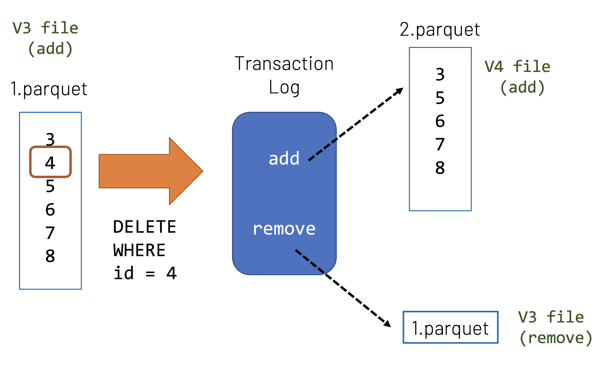
Figure 2-6. Delete data involves add file per V3 and V4
Notice how the remove.path value is the same file as the preceding version 3 file. But as you can see from the following query, a new file is created.
%python# Add Informationj4.select("add.path").where("add is not null").show(20,False)
%scala// Add Informationj4.select("add.path").where("add is not null").show(20,False)
-- Result+-------------------------------------------------------------------+|path |+-------------------------------------------------------------------+|part-00000-68bf51ea-6e00-4591-b267-62fcd36602ed-c000.snappy.parquet|+-------------------------------------------------------------------+
If you query this file, observe that it contains only the expected values of {3, 5-8}.
%python# Read the V4 added filespark.read.parquet("/table_delta/part-00000-68bf51ea-6e00-4591-b267-62fcd36602ed-c000.snappy.parquet").show()%python//ReadtheV4addedfilespark.read.parquet("/table_delta/part-00000-68bf51ea-6e00-4591-b267-62fcd36602ed-c000.snappy.parquet").show()
-- Result+---+| id|+---+| 8|| 3|| 6|| 9|| 7|+---+
To reiterate, instead of deleting the value 4 from the original file, instead Delta is creating a new file with the values not deleted (in this case) and keeping the old file in place.
Let’s go back in time
What you’re seeing here is multiversion concurrency control (MVCC) in action where there are two separate files associated with two different table versions. But how about if you do want to query the previous data? Well, this is an excellent segue to Delta time travel options.
Time Travel
In Chapter 1 we unpacked what was happening with the transaction log to provide ACID transactional semantics. In the previous section, we unpacked what was happening with the data files in relation to the transaction log in light of Delta transactional protocol with particular focus on multiversion concurrency control (MVCC). An interesting byproduct of MVCC is that all of the files from previous transactions still reside and are accessible in storage. That is, the positive byproduct of the implementation of MVCC in Delta is data versioning or time travel.
From a high-level, Delta automatically versions the big data that you store in your data lake, and you can access any historical version of that data. This temporal data management simplifies your data pipeline by making it easy to audit, roll back data in case of accidental bad writes or deletes, and reproduce experiments and reports. You can standardize on a clean, centralized, versioned big data repository in your own cloud storage for your analytics.
Common Challenges with Changing Data
Data versioning is an important tool to ensure data reliability to address common challenges with changing data.
- Audit data changes
-
Auditing data changes is critical from both in terms of data compliance as well as simple debugging to understand how data has changed over time. Organizations moving from traditional data systems to big data technologies and the cloud struggle in such scenarios.
- Reproduce experiments & reports
-
During model training, data scientists run various experiments with different parameters on a given set of data. When scientists revisit their experiments after a period of time to reproduce the models, typically the source data has been modified by upstream pipelines. Lot of times, they are caught unaware by such upstream data changes and hence struggle to reproduce their experiments. Some scientists and organizations engineer best practices by creating multiple copies of the data, leading to increased storage costs. The same is true for analysts generating reports.
- Rollbacks
-
Data pipelines can sometimes write bad data for downstream consumers. This can happen because of issues ranging from infrastructure instabilities to messy data to bugs in the pipeline. For pipelines that do simple appends to directories or a table, rollbacks can easily be addressed by date-based partitioning. With updates and deletes, this can become very complicated, and data engineers typically have to engineer a complex pipeline to deal with such scenarios.
Working with Time Travel
Delta’s time travel capabilities simplify building data pipelines for the preceding use cases which we will further explore in the following sections. As noted previously, as you write into a Delta table or directory, every operation is automatically versioned. You can access the different versions of the data two different ways:
-
Using a timestamp
-
Using a version number
In the following examples, we will use the generated TPC-DS dataset so we can work with the following example customer table (customer_t1). To review the historical data, run the DESCRIBE HISTORY command.
%sqlDESCRIBEHISTORYcustomer_t1;
The following results are an abridged version of the table initially focusing only on the version, timestamp, and operation columns.
-- Abridged Results+-------+-------------------+---------+|version| timestamp|operation|+-------+-------------------+---------+| 19|2020-10-30 18:15:03| WRITE|| 18|2020-10-30 18:10:47| DELETE|| 17|2020-10-30 08:41:47| WRITE|| 16|2020-10-30 08:37:29| DELETE|| 15|2020-10-30 05:34:29| RESTORE|| 14|2020-10-30 02:50:07| WRITE|| 13|2020-10-30 02:37:17| DELETE|| 12|2020-10-30 02:31:36| WRITE|| 11|2020-10-28 23:33:34| DELETE|+-------+-------------------+---------+
The following sections describe the various techniques to work with your versioned data.
Using a timestamp
You can provide the timestamp or date string as an option to the DataFrame reader using the following syntax.
%sql-- Query metastore-defined Delta table by timestampSELECT*FROMmy_tableTIMESTAMPASOF"2019-01-01"SELECT*FROMmy_tableTIMESTAMPASOFdate_sub(current_date(),1)SELECT*FROMmy_tableTIMESTAMPASOF"2019-01-01 01:30:00.000"-- Query Delta table by file path by timestampSELECT*FROMdelta.`<path-to-delta>`TIMESTAMPASOF"2019-01-01"SELECT*FROMdelta.`<path-to-delta>`TIMESTAMPASOFdate_sub(current_date(),1)SELECT*FROMdelta.`<path-to-delta>`TIMESTAMPASOF"2019-01-01 01:30:00.000"
%python# Load into Spark DataFrame from Delta table by timestamp(df=spark.read.format("delta").option("timestampAsOf","2019-01-01").load("/path/to/my/table"))
%scala// Load into Spark DataFrame from Delta table by timestampvaldf=spark.read.format("delta").option("timestampAsOf","2019-01-01").load("/path/to/my/table")
Specific to the customer_t1 table, the following queries will allow you to query by two different timestamps. The following SQL queries will use the metastore-defined Delta table syntax.
%sql-- Row count as of timestamp t1SELECTCOUNT(1)FROMcustomer_t1TIMESTAMPASOF"2020-10-30T18:15:03.000+0000"-- Row count as of timestamp t2SELECTCOUNT(1)FROMcustomer_t1TIMESTAMPASOF"2020-10-30T18:10:47.000+0000"
%python# timestampst1="2020-10-30T18:15:03.000+0000"t2="2020-10-30T18:10:47.000+0000"DELTA_PATH="/demo/customer_t1"># Row count as of timestamp t1(spark.read.format("delta").option("timestampAsOf",t1).load(DELTA_PATH).count())# Row count as of timestamp t2(spark.read.format("delta").option("timestampAsOf",t2).load(DELTA_PATH).count())
%scala// timestampsvalt1="2020-10-30T18:15:03.000+0000"valt2="2020-10-30T18:10:47.000+0000"valDELTA_PATH="/demo/customer_t1"// Row count as of timestamp t1spark.read.format("delta").option("timestampAsOf",t1).load(DELTA_PATH).count()// Row count as of timestamp t2spark.read.format("delta").option("timestampAsOf",t2).load(DELTA_PATH).count()
The preceding queries have the following results below.
| Timestamp | Row Count |
| 2020-10-30T18:15:03.000+0000 | 65000000 |
| 2020-10-30T18:10:47.000+0000 | 58500000 |
If the reader code is in a library that you don’t have access to, and if you are passing input parameters to the library to read data, you can still travel back in time for a table by passing the timestamp in yyyyMMddHHmmssSSS format to the path:
spark.read.format("delta").load(<path-to-delta>@yyyyMMddHHmmssSSS)
For example, to query for the timestamp 2020-10-30T18:15:03.000+0000, use the following Python and Scala syntax.
%python# Delta table base pathBASE_PATH="/demo/customer_t1"# Include timestamp in yyyyMMddHHmmssSSS formatDELTA_PATH=BASE_PATH+"@20201030181503000"# Get row count of the Delta table by timestamp using @ parameterspark.read.format("delta").load(DELTA_PATH).count()
%scala// Delta table base pathvalBASE_PATH="/demo/customer_t1"// Include timestamp in yyyyMMddHHmmssSSS formatvalDELTA_PATH=BASE_PATH+"@20201030181503000"// Get row count of the Delta table by timestamp using @ parameterspark.read.format("delta").load(DELTA_PATH).count()
Using a version number
In Delta, every write has a version number, and you can use the version number to travel back in time as well.
%sql-- Query metastore-defined Delta table by versionSELECTCOUNT(*)FROMmy_tableVERSIONASOF5238SELECTCOUNT(*)FROMmy_table@v5238-- Query Delta table by file path by versionSELECTcount(*)FROMdelta.`/path/to/my/table@v5238`
%python# Query Delta table by version using versionAsOf(df=spark.read.format("delta").option("versionAsOf","5238").load("/path/to/my/table"))# Query Delta table by version using @ parameter(df=spark.read.format("delta").load("/path/to/my/table@v5238"))
%scala// Query Delta table by version using versionAsOfvaldf=spark.read.format("delta").option("versionAsOf","5238").load("/path/to/my/table")// Query Delta table by version using @ parametervaldf=spark.read.format("delta").load("/path/to/my/table@v5238")
Specific to the customer_t1 table, the following queries will allow you to query by two different versions. The following SQL queries will use the metastore-defined Delta table syntax.
%sql-- Query metastore-defined Delta table by version 19SELECTCOUNT(1)FROMcustomer_t1VERSIONASOF19SELECTCOUNT(1)FROMcustomer_t1@v19-- Query metastore-defined Delta table by version 18SELECTCOUNT(1)FROMcustomer_t1VERSIONASOF18SELECTCOUNT(1)FROMcustomer_t1@v18
%python# Delta table base pathDELTA_PATH="/demo/customer_t1"# Row count of Delta table by version 19(spark.read.format("delta").option("versionAsOf",19).load(DELTA_PATH).count())# Row count of Delta table by version 18(spark.read.format("delta").option("versionAsOf",18).load(DELTA_PATH).count())# Row count of Delta table by @ parameter for version 18(spark.read.format("delta").load(DELTA_PATH+"@v18").count())
%scala#DeltatablebasepathvalDELTA_PATH="/demo/customer_t1"#RowcountofDeltatablebyversion19spark.read.format("delta").option("versionAsOf",19).load(DELTA_PATH).count()#RowcountofDeltatablebyversion18spark.read.format("delta").option("versionAsOf",18).load(DELTA_PATH).count()#RowcountofDeltatableby@parameterforversion18spark.read.format("delta").load(DELTA_PATH+"@v18").count()
The preceding queries have the following results below.
| Version | Row Count |
| 19 | 65000000 |
| 18 | 58500000 |
Time travel use cases
In this section, we will focus on how to apply time travel for various use cases, and why it’s important to them.
- Debug
-
To troubleshoot the ETL pipeline or data quality issues, or to fix the accidental broken data pipelines. This is the most common use case for time travel and we will be exploring this use case throughout the book.
- Governance and Auditing
-
Time travel, offers a verifiable data lineage that is useful for governance, audit and compliance purposes. As the definitive record of every change ever made to a table, you can trace the origin of an inadvertent change or a bug in a pipeline back to the exact action that caused it. If your GDPR pipeline job had a bug that accidentally deleted user information, you can fix the pipeline. Retention and vacuum allows you to act on Data subject requests well within the timeframe.
- Rollbacks
-
Time travel also makes it easy to do rollbacks in case of bad writes. Due to a previous error, it may be necessary to rollback to a previous version of the table before continuing forward with data processing.
- Reproduce experiments & reports
-
Time travel also plays an important role in machine learning and data science. Reproducibility of models and experiments is a key consideration for data scientists, because they often create 100s of models before they put one into production, and in that time-consuming process would like to go back to earlier models.
- Pinned view of a continuously updating Delta table across multiple downstream jobs
-
With AS OF queries, you can now pin the snapshot of a continuously updating Delta table for multiple downstream jobs.
- Time series analytics
-
Time travel simplifies time series analytics. You can use
timestampandAs Ofqueries to extract meaningful statistics associated with the selected data points and shift in associated variables over time.
Next we will provide further details for each use case. Note, we will cover more advanced use cases which include time travel in chapter 14.
Use Case: Governance and Auditing
The use case of Governance described here is about protecting people’s information in regards to GDPR (General Data Protection Regulation) and CCPA (California Consumer Privacy Act). The role of governance is to set the direction of protecting information in the form of policies, standards, and guidelines.
One of the most common scenarios surrounding governance to protect people’s information is the need to perform a delete request as part of any GPDR or CCPA compliance. What that means for data engineers is that you need to locate the records from your Delta Lake and delete it within the specified time period. Users can run DESCRIBE HISTORY to see metadata around the changes that were made. An example of this scenario is how Starbucks implements governance, risk and control for their Delta lake.
Let’s dive further in the simplified governance use case (see Figure 3-x).
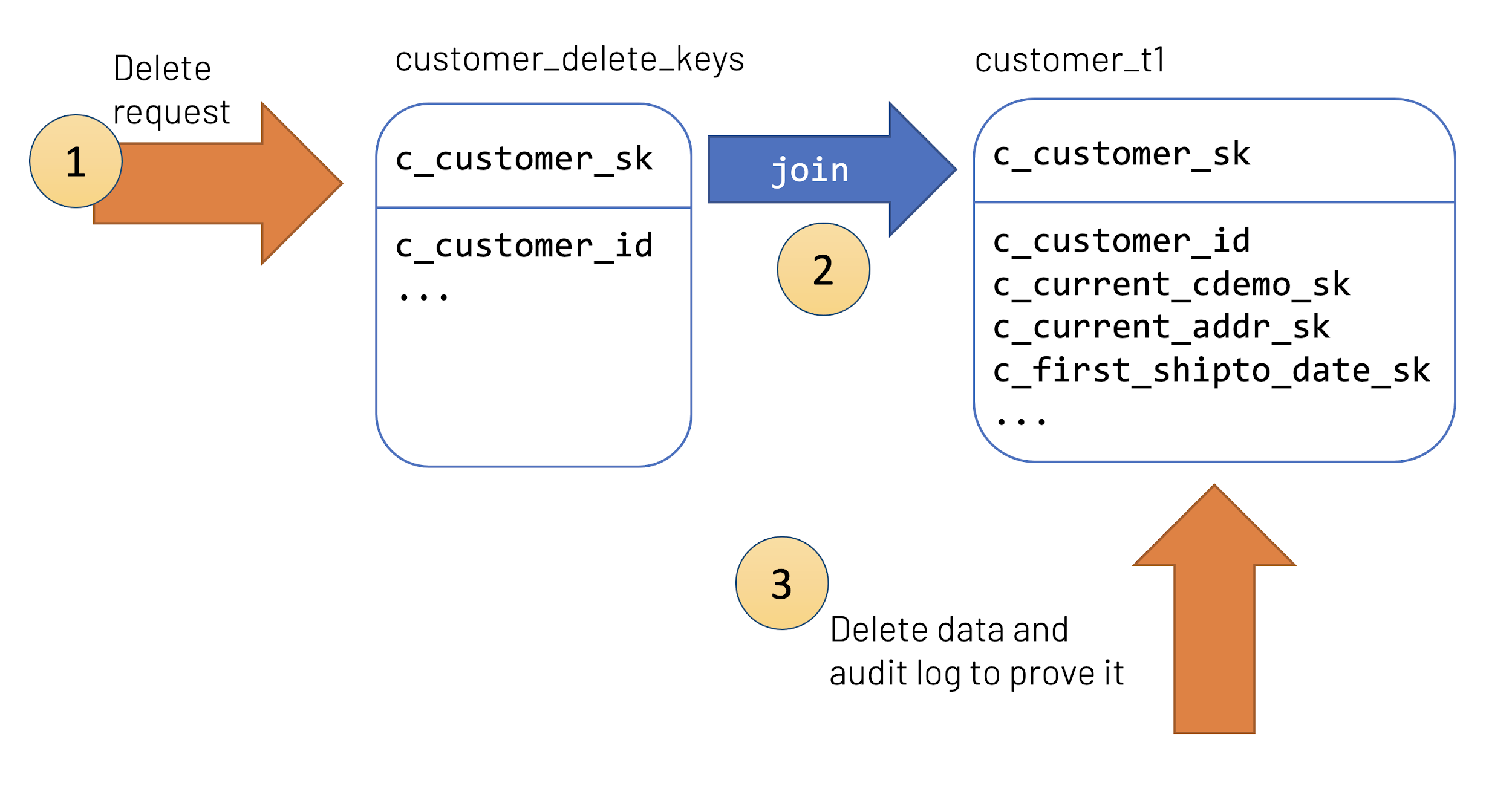
Figure 2-7. Simplified governance use case with time travel
-
A delete request is recorded in the system where the user has requested that their information be removed from the data lake. This information is often recorded in its own table or store for auditing and lineage purposes.
-
This table (
customer_delete_keys) will need to join with the customer table (customer_t1) to identify which users in the table need to be removed. -
You will then delete this data from the system to address this delete request.
With Delta Lake, you can achieve the above listed goals by running the following steps. You can also use this notebook for the whole code.
Identify users that need to be removed
As noted earlier, the customer_delete_keys table contains the set of customer keys that need to be removed. To review the table, run the following query.
%sqlSELECT*FROMcustomer_delete_keys
%python# Query table using metastore defined tablesql("SELECT * FROM customer_delete_keys").show()# Query table from file pathspark.read.format(“delta”).load("/customer_delta_keys").show()
%scala// Query table using metastore defined tablesql("SELECT * FROM customer_delete_keys”).show()// Query table from file pathspark.read.format(“delta”).load("/customer_delta_keys").show()
Note
Note, going forward in this section, we will only use metastore-defined SQL queries. In Python and Scala, you can also use the syntax:
sql("<sql-statement-here>").show()
A partial result of the above queries can be seen in the output below.
+----------------+-------------+
|   c_customer_id|c_customer_sk|
+----------------+-------------+
|AAAAAAAAKHJBCKBA|     27400570|
|AAAAAAAAFIJBCKBA|     27400581|
|AAAAAAAAGIJBCKBA|     27400582|
|AAAAAAAAHIJBCKBA|     27400583|
|...             |          ...|
+----------------+-------------+
The following SQL query will allow you to quickly identify the records that need to be removed from customer_t1.
%sql-- Identify the recordsSELECTCOUNT(*)FROMcustomer_t1WHEREc_customer_idIN(SELECTc_customer_idFROMcustomer_delete_keys)
-- Result+--------+|count(1)|+--------+| 6500000|+--------+
Delete the identified users
Once we have identified the matches, you can now go ahead and use the DELETE function to remove those records from the Delta table.
%sql-- Delete identified recordsDELETEFROMcustomer_t1WHEREc_customer_idIN(SELECTc_customer_idFROMcustomer_delete_keys)
Fortunately this process is pretty straightforward as you can remove the SELECT clause and replace it with a DELETE clause. You can validate this by reviewing the transaction log via the DESCRIBE HISTORY command (See Figure 3-x).
%sqlDESCRIBEHISTORYcustomer_t1;

Figure 2-8. Reviewing history after fulfilling GDPR delete request
Below is the transposed table of the DELETE transaction so we can inspect information.
| Column Name | Column Value |
| version | 13 |
| operation | DELETE |
| operationParameters | [predicate -> ["exists(t1.`c_customer_id`)"]] |
| operationMetrics | [ numRemovedFiles -> 23, numDeletedRows -> 6500000, numAddedFiles -> 100, numCopiedRows -> 42250002 ] |
Let’s dive further in the audit use case
Auditor’s role is to review and inspect that delivery conforms to those guidelines. For auditing purposes, you can review the Delta transaction log which tracks all of the changes to your Delta table. In this case, for version 13 of the table:
-
Through the
operationcolumn, aDELETEactivity was recorded. -
The
operationParametersdenote how the delete occurred, i.e. the delete was done by thec_customer_idcolumn. -
From an auditing perspective, the important callout is the 6,500,000 rows deleted (
numDeletedRows) underoperationMetrics. This allows us to determine the magnitude of impact on the records.
Delete is a tombstone
It is important to note that when a DELETE is executed on a Delta table, the most current version of the table no longer reads this data, as it is explicitly excluded. If you recall earlier in the chapter, the Remove column of the transaction log will contain the files that no longer should be included.
For some organizations, this meets their compliance requirements as the data is no longer accessible by default. But depending on your legal requirements, there are additional considerations:
-
If the data must be removed immediately, run the
VACUUMcommand to remove the data files -
Instead of deleting,
UPDATEthe data (e.g. update the name column with some other value such as a GUID) so you can keep the associated IDs without having any personally identifiable information. -
Place personally identifiable information into a separate table so that GDPR delete requests would result in only updating or deleting the information from this demographics table with little to no impact on your fact data.
It is important to note that this example is showcasing a simplified governance use case. You will need to work with your legal department to determine your actual requirements. The key takeaway for our discussion here is that Delta Lake time travel allows you to safely remove data from your Delta Lake, reverse it in case there are mistakes, and track the progress through the Delta Lake transaction log.
For more information on governance:
Use Case: Rollbacks
Time travel also makes it easy to do rollbacks so you can reset your data to a previous snapshot. If a user accidentally inserted new data or your pipeline job inadvertently deleted user information, you can easily fix it by restoring the previous version of the table.
The following code sample takes our existing customer_t1 table and restores it to version 17. Let’s start by reviewing the history of our table.
%sqlDESCRIBEHISTORYcustomer_t1
--- abridged results+-------+---------+---------------------------------------------+|version|operation|operationParameters |+-------+---------+---------------------------------------------+|18 |DELETE |[predicate -> ["exists(t1.`c_customer_id`)"]]||17 |WRITE |[mode -> Overwrite, partitionBy -> []] |+-------+---------+---------------------------------------------+
Insert and overwrite
To rollback, what we really are doing is that once we identify which version of the table we want to travel back to, we will load that version using as of. Behind the scenes, delta inserts it as a new version and overwrites the latest snapshot. In this scenario, you can see from the abridged history results that version 18 of the table contains a DELETE operation that we want to rollback from. The following code allows you to perform the rollback.
%python# Restore customer_t1 table to Version 17># Load Version 17 data using dfdf=spark.read.format("delta").option("versionAsOf","17").load("/customer_t1")# Overwrite Version 17 as the current versiondf.write.format("delta").mode("overwrite").save("/customer_t1")
%scala// Restore customer_t1 table to Version 17// Load Version 17 data using dfvaldf=spark.read.format("delta").option("versionAsOf","17").load("/customer_t1")// Overwrite Version 17 as the current versiondf.write.format("delta").mode("overwrite").save("/customer_t1")
You can validate this by either querying the data or reviewing the table history. The following is how you would do this using SQL.
%sql-- Get the row counts between two table versions and calculate the differenceSELECTa.v19_cnt,b.v17_cnt,a.v19_cnt-b.v17_cntASdifferenceFROM-- Get V19 row count(SELECTCOUNT(1)ASv19_cntFROMcustomer_t1VERSIONASOF19)aCROSSJOIN-- Get V17 row count(SELECTCOUNT(1)ASv17_cnt>FROMcustomer_t1VERSIONASOF17)b
-- Result+--------+--------+----------+| v19_cnt| v17_cnt|difference|+--------+--------+----------+|65000000|65000000| 0|+--------+--------+----------+
A comparable code can be written in Python and Scala versions as shown below .
%python# Get V19 row countv19_cnt=sql("SELECT COUNT(1) AS v19_cnt FROM customer_t1 VERSION AS OF 19").first()[0]# Get V17 row countv17_cnt=sql("SELECT COUNT(1) AS v17_cnt FROM customer_t1 VERSION AS OF 17").first()[0]# Calculate the difference("Difference in row count between v19 and v17:%s"%(v19_cnt-v17_cnt))
%scala// Get V19 row countvalv19_cnt=sql("SELECT COUNT(1) AS v19_cnt FROM customer_t1 VERSION AS OF 19").first()(0).toString.toInt// Get V19 row countvalv17_cnt=sql("SELECT COUNT(1) AS v17_cnt FROM customer_t1 VERSION AS OF 17").first()(0).toString.toInt// Calculate the difference("Difference in row count between v19 and v17: "+(v19_cnt-v17_cnt))
You will get the same result for both the Python and Scala examples.
-- ResultDifference in row count between v19 and v17: 0
You can also validate the restore by reviewing the table history; note that there is now version 19 that records the overwrite statement.
%sql
DESCRIBE HISTORY customer_t1
--- abridged results+-------+---------+---------------------------------------------+|version|operation|operationParameters |+-------+---------+---------------------------------------------+|19 |WRITE |[mode -> Overwrite, partitionBy -> []] ||18 |DELETE |[predicate -> ["exists(t1.`c_customer_id`)"]]||17 |WRITE |[mode -> Overwrite, partitionBy -> []] |+-------+---------+---------------------------------------------+
RESTORE command
Note, if you are using Databricks, this step will be a little easier when restoring with at least DBR 7.4 with the RESTORE command. You can perform the same steps as above with a single atomic command.
%sql-- Restore table as of version 17RESTOREcustomer_t1VERSIONASOF17
In addition to the previous queries comparing the count of two different versions, once you run the RESTORE, additional information gets stored within the transaction log which are shown under the operationMetrics column map.
%sqlDESCRIBEHISTORYcustomer_t1
-- Abridged results+-------+---------+---------------------------------------------+|version|operation|operationParameters |+-------+---------+---------------------------------------------+|20 |RESTORE |[version -> 17, timestamp ->]||19 |WRITE |[mode -> Overwrite, partitionBy -> []] ||18 |DELETE |[predicate -> ["exists(t1.`c_customer_id`)"]]||17 |WRITE |[mode -> Overwrite, partitionBy -> []] |+-------+---------+---------------------------------------------+
Note
We are highlighting the record 20 from our output above for the restore operation of the delta table to explain the operationMetrics restore-based parameters.
{"numRestoredFiles": "31", "removedFilesSize": "3453647999", "numRemovedFiles": "31", "restoredFilesSize": "3453647999", "numOfFilesAfterRestore": "31", "tableSizeAfterRestore": "3453647999"}
For more information about the RESTORE command, see Restore a Delta table.
Time travel considerations
We need to keep additional considerations in mind with respect to time travel.
Data retention:
-
One very important thing to remember is Data retention. You can only travel back so far depending on what time limits we set and how much data is retained.
-
To time travel to a previous version, you must retain both the log and the data files for that version.
Vacuum:
-
The ability to time travel back to a version older than the retention period is lost after running vacuum.
-
By default, `vacuum()` retains all the data needed for the last 7 days.
-
When you run the
vacuumwith specified retention of 0 hours, it will throw an exception.-
Delta protects you by giving this warning to save you from permanent changes to your data or if a downstream reader or application is referencing your table.
-
If you are certain that there are no operations being performed on this table, such as insert/upsert/delete/optimize, then you may turn off this check by setting:
spark.databricks.delta.retentionDurationCheck.enabled = false
-
-
VACUUMdoesn’t clean up log files; log files are automatically cleaned up after checkpoints are written. -
Another note to satisfy the delete requirement is that you also need to delete it from your blob storage. So as a best practice, whenever the ETL pipeline is set you should apply the retention policy from the start itself so you don’t have to worry later.
Summary
In this chapter, we focussed on a powerful benefit of the MVCC (Multi-Version Concurrency Control) implementation of Delta, that enables users to have the benefit of data versioning or time travel. In addition to showing common challenges with changing data, we explained the Delta time machine and its properties, how time travel works and what operations you can perform while traveling back in time.
As alluded to earlier in the chapter, time travel allows developers to debug what happened with their Delta table, improving developer productivity tremendously. One of the common reasons developers need to debug their table is due to data modification such as delete, update, and merge. This brings us to our next chapter, Chapter 4: Data Modifications in Delta tables.