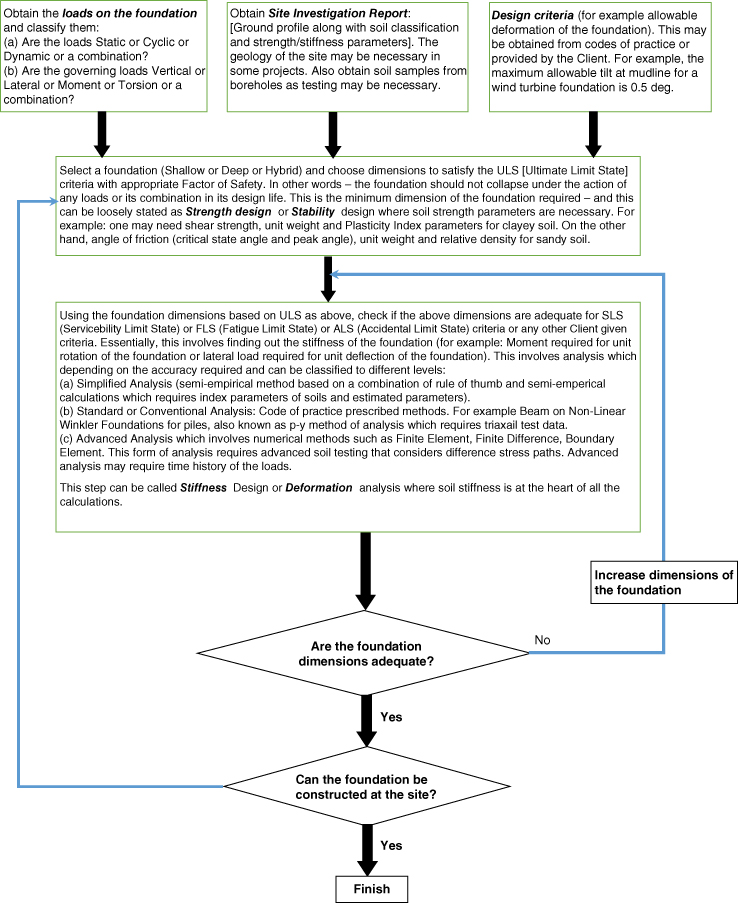
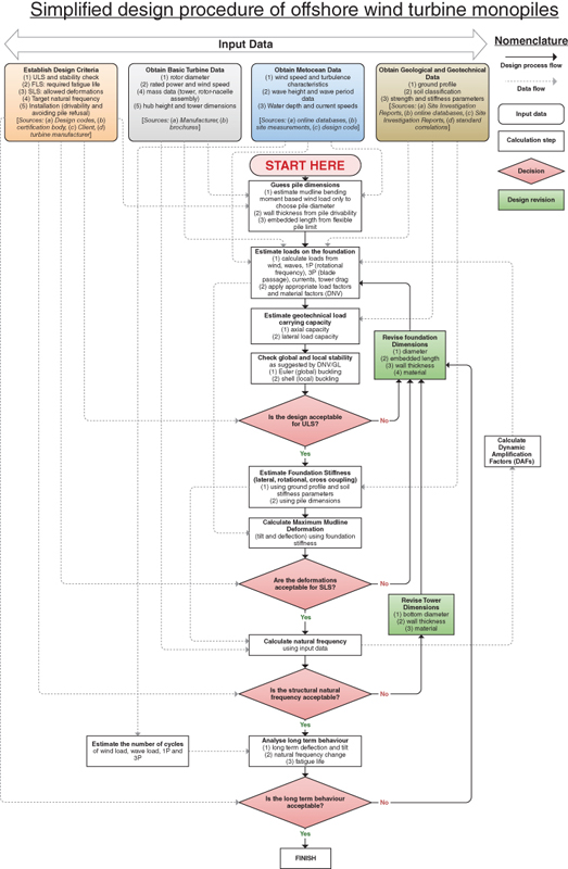
Guess Initial Pile Dimensions
The initial pile dimensions are Chapter 2 . A spreadsheet can be used to carry out these calculations. The wind load on the rotor can already be calculated in the first step; however, the wave loading depends on the monopile diameter, and therefore it can only be calculated after the initial pile dimensions are available.
Calculate Highest Wind Load
The wind load for ULS is determined from the 50‐year extreme operating gust (EOG ), which is assumed to produce the highest single occurrence wind load; this is wind scenario (U‐3), see Section 2.6.1 for further details. The procedure outlined in Section 2.6.2 (Chapter 2 ) is used to estimate the wind load for this scenario. First the EOG wind speed is calculated using data from Tables 6.13 and 6.14 .
Using this, the total wind load is estimated as
6.38
and using the water depth S =25 [m]z hub
6.39 Applying a load factor of γ L U R
Calculate Initial Pile Dimensions
The initial value of wall thicknes2005 ) as
6.40 This wall thickness value may not necessarily provide sufficient stability to avoid local or global buckling of the pile, or to ensure that the pile can be driven into the seabed with the simplest installation method avoiding pile tip damage leading to early refusal. Therefore, these issues need to be addressed separately, as well as fatigue design of the pile, which may require additional wall thickness. Figure 6.16 shows the wall thickness for installed offshore wind turbines of different monopile diameters. As can be seen, some piles have wall thicknesses significantly higher than the API‐required thickness. For details on buckling‐related issues (global buckling, avoiding local pile buckling or propagating pile tip damage due to installation), see Bhattacharya et al. (2005 ), Aldridge et al. (2005 ). For practical reasons, the wall thickness is typically chosen based on standard plate thickness values to optimise manufacturing.
Figure 6.16 Table 6.16 .
Using the pile thickness formula of API (2005 ) given by Eq. (6.40 ), the following can be written for the area moment of inertia of the pile cross section:
6.41 The following has to be satisfied to avoid pile yield with material factor γ M
6.42
from which the required diameter is determined as
6.43 This results in an initial pile diameter of D P t P
The embedded length is determined next.
The formula of Poulos and Davis (1980 )
6.44 The initial pile dimensions are then
6.45 Estimate Loads on the Foundation
Now that an initial guess for the pile dimensions is available, the wave load can be calculated. For the combination of wind and wave loading, many load cases are presented in design standards. Five conservative load cases are considered in Table 6.17 . Among the potential severe load cases not covered by these scenarios are shutdown events of the wind turbine, as these situations require detailed data about the wind turbine (rotor, blades, control system parameters, generator, etc.), but are likely to provide a lower foundation load than the scenarios in Table 6.17 .
Calculate Wind Loads (Other Wind Scenarios)
The wind loads on the structure are independent of the substructure diameter, and therefore the wind loads can be evaluated before the pile and substructure design are available. Section 2.6.2 is used to determine the turbulent wind speed component and through that the thrust force and overturning moment. Table 6.17 summarises the important parameters and presents the wind loads for the different wind scenarios. Note that the mean of the maximum and minimum loads are not equal to the mean force without turbulent wind component. This is because the thrust force is proportional to the square of the wind speed.
Calculate Critical Wave Loads
The wave load is first calculated only for the most severe wave scenarios used for Load Cases E‐2 and E‐3, i.e. wave scenario (W‐2) and (W‐4), the 1‐year and 50‐year extreme wave height s (EWH s). The methodology described in Section 2.6.3 is used to calculate the wave loading, and the substructure diameter, which in this case is D S Table 6.16 . The 1‐year equivalents are calculated following (DNV 2014 ) from the 50‐year significant wave height according to
6.46 Table 6.16 Pile diameters and wall thicknesses of monopiles shown in Figure 6.16 .
#
Wind farm and turbine
Pile diameter [m]
Wall thickness range [mm]
1
Lely, Netherlands, A2 turbine
3.2
35
–
35
2
Lely, Netherlands, A3 turbine
3.7
35
–
35
3
Irene Vorrink, Netherlands
3.515
35
–
35
4
Blyth, England, UK
3.5
40
–
40
5
Kentish Flats, England, UK
4.3
45
–
45
6
Barrow, England, UK
4.75
45
–
80
7
Thanet, England, UK
4.7
60
–
60
8
Belwind, Belgium
5
50
–
75
9
Burbo Bank, England, UK
4.7
45
–
75
10
Walney, England, UK
6
60
–
80
11
Gunfleet Sands, England, UK
5
35
–
50
12
London Array, England, UK
4.7
50
–
75
13
Gwynt y Mór, Wales, UK
5
55
–
95
14
Anholt, Denmark
5.35
45
–
65
15
Walney 2, England, UK
6.5
75
–
105
16
Sheringham Shoal, England, UK
5.7
60
–
60
17
Butendiek, Germany
6.5
75
–
90
18
DanTysk, Germany
6
60
–
126
19
Meerwind Ost/Sud, Germany
5.5
50
–
65
20
Northwind, Belgium
5.2
55
–
70
21
Horns Rev, Denmark
4
20
–
50
22
Egmond aan Zee, Netherlands
4.6
40
–
60
23
Gemini, Netherlands
5.5
59
–
73
24
Gemini, Netherlands
7
60
–
85
25
Princess Amalia, Netherlands
4
35
–
79
26
Inner Dowsing, England, UK
4.74
50
–
75
27
Rhyl Flats, Wales, UK
4.72
50
–
75
28
Robin Rigg, Scotland, UK
4.3
50
–
75
29
Teesside, England, UK
4.933
70
–
90
Table 6.17 Load and overturning moment for wind scenarios (U‐1) – (U‐4).
Parameters
Symbol [unit]
Wind scenario (U‐1)
Wind scenario (U‐2)
Wind scenario (U‐3)
Wind scenario (U‐4)
Standard deviation of wind speed
σ U 2.63
3.96
–
–
Standard deviation in f>f1P
0.73
1.22
–
–
Turbulent wind speed component
u [m/s] 0.94
2.44
8.1
4.86
Maximum force in load cycle
Fmax [MN] 0.68
0.84
1.63
0.40
Minimum force in load cycle
Fmin [MN] 0.49
0.37
0.39
0.25
Mean force without turbulence
Fmean [MN] 0.58
0.58
0.58
0.28
Maximum moment in load cycle
Mmax [MN]75.8
94.4
182.8
44.6
Minimum moment in load cycle
Mmin [MN]55.4
41.4
43.7
28.1
Mean moment without turbulence
Mmean [MN]65.2
65.2
65.2
31.3
Table 6.18 Wave heights and wave periods for different wave scenarios.
Parameters
Symbol [unit]
Wave scenario (W‐1)
Wave scenario (W‐2)
Wave scenario (W‐3)
Wave scenario (W‐4)
Wave height
H 5.3
10
6.6
12.4
Wave period
T 8.1
11.2
9.1
12.5
Section 5.6 is used to determine the 1‐year maximum wave height and period:
6.47 The wave heights and wave periods are summarised for all wave scenarios (W‐1) to (W‐4) in Table 6.18 .
The maximum of the inertia load occurs at the time instant t =0η =0t =T m η =H m
The maximum drag and inertia loads for wave scenario (W‐2) with the 1‐year EWH are then
6.48 The maxima of the wave loads and moments may be conservatively taken as
6.49 Similarly, for the 50‐year EWH in wave scenario (W‐4) the drag and inertia loads are given as
6.50
and the maxima of the wave load
6.51 Table 6.19 ULS load combinations.
Load
Extreme Wave Scenario (E‐2)ETM (U‐2) and 50‐year EWH (W‐4)
Extreme Wind Scenario (E‐3)EOG at UR (U‐3) and 1‐year EWH (W‐2)
Maximum wind load [MN]
0.84
1.63
Maximum wind moment [MNm]
94.4
182.6
Maximum wave load [MN]
2.77
2.13
Maximum wave moment [MNm]
67.7
53.8
Total load [MN]
3.61
3.79
Total overturning moment [MNm]
162.1
236.4
Load Combinations for ULS
The most severe load cases in Table 6.19 for ULS design are E‐2 and E‐3, the extreme wave scenario (50‐year EWH) combined with extreme turbulence model (ETM) and the extreme operational gust (EOG) combined with the yearly maximum wave height (1‐year EWH). A partial load factor of γ L 2014 ) and IEC (2009a ). Table 6.19 shows the ULS loads for the two load combinations, and it is clear from the table that for this particular example the driving scenario is (E‐3), since the overturning moment is dominated by the wind load.
The new total loads in Table 6.19 are used to recalculate the required foundation dimensions. This will result in an iterative process of finding the necessary monopile size for the ULS load, which can be easily solved in a spreadsheet. The analysis results in the following dimensions:
6.52 The stability analysis has to be carried out following the Germanischer Lloyd (2005 ) Chapter 6 on the design of steel support structures.
Estimate Geotechnical Load Carrying Capacity
In typical scenarios, the limiting case for maximum lateral load results from the yield strength of the pile. However, a check has to be performed to make sure that the foundation can take the load, that is, that the soil does not fail at the ULS load. Based on the standard methods outlines in Section 5.3.3.4 , the ultimate horizontal load bearing capacity and the ultimate moment capacity of the pile are established as F R MN M R MNm
In terms of vertical load, it is expected that failure due to lateral load occurs first and that stability under lateral load ensures the pile's ability to take the vertical load imposed mainly by the deadweight of the structure. The analysis of vertical load‐carrying capacity is therefore omitted here, but has to be performed in actual design.
Estimate Deformations and Foundation Stiffness
Many methods as explained in Examples can be used to evaluate foundation. In this example, the method by Poulos and Davis (1980 ) is used. The method requires the modulus of subgrade reaction for cohesive (clayey) and the coefficient of subgrade reaction for cohesionless (sandy) soils. The upper layers are dominant for the calculation of deflections and stiffness. The sand and silt layers were approximated here with the coefficient of subgrade reaction n h MN /m 3 ]1980 ) formulae for flexible piles in medium sand.
6.53
and their values are
6.54 The deflections and rotations are calculated following equations in Chapter 5 and calculations presented in
6.55 The pile tip deflection is acceptable but the rotation exceeds 0.5°.
Again, an iterative process is necessary by which the necessary pile dimensions are obtained. This can be done by the following iterative steps:
The foundation dimensions are increased.
Recalculate the foundation loads.
The foundation stiffness parameters are recalculated based on appropriate equations.
The mudline deformations are recalculated.
The process is repeated until the deflection and rotation are both below the allowed limit.
A spreadsheet can be used to easily obtain the necessary dimensions:
6.56
and the deformations are now
6.57 Calculate Natural Frequency and Dynamic Amplification Factors
The natural frequency is calculated following the method given in Chapter 5 and developed in Arany et al. (2015a ) and Arany et al. (2016 ). The first natural frequency and the damping of the first mode in the along‐wind and cross‐wind directions are used to obtain the DAFs that affect the structural response.
Calculate Natural Frequency
The structural natural frequency of the turbine‐tower‐substructure‐foundation system is given by f 0 =C L C R C S f FB C S C R C L
6.58 The substructure flexibility coefficient C S L S m ]χ =E T I T E P I P ψ =L S L T
6.59 The nondimensional foundation stiffnesses are calculated:
6.60
and the foundation flexibility coefficients are calculated:
6.61 The natural frequency is then
6.62 This is acceptable, as the condition was that f 0 >0.24[Hz]
Calculate Dynamic Amplification Factors
The dynamic amplification of the wave loading is calculated using the peak wave frequency and an assumed damping ratio. The total damping ratios for the along‐wind (x ) and cross‐wind (y ) directions are chosen conservatively as 3% and 1%, respectively. The along‐wind damping is larger due to the significant contribution of aerodynamic damping. In real cases, the aerodynamic damping depends on the wind speed, and the along‐wind value may be between 2% and 10%. The chosen value is conservatively small for the relevant wind speed ranges, see e.g. Camp et al. (2004 ), or the discussion on damping in Arany et al. (2016 ). The DAFs are calculated as
6.63
where f f 0 ξ Table 6.20 . The difference in DAFs in the along‐wind (x ) and cross‐wind (y ) directions is apparently negligible for this example, and in Table 6.21 the higher value is used when loads with DAF are calculated.
Table 6.20 Dynamic amplification factors and wave loads.
Parameters
Symbol [unit]
Wave scenario (W‐1)
Wave scenario (W‐2)
Wave scenario (W‐3)
Wave scenario (W‐4)
Wave period
T [s] 8.1
11.2
9.1
12.5
Wave frequency
f [Hz] 0.123 0.089 0.110 0.080
Dynamic amplification – along‐wind
DAF x 1.285 1.131 1.215 1.103
Dynamic amplification – cross‐wind
DAF y 1.288 1.133 1.215 1.104
Total wave load
F w 1.41
2.77
1.77
3.56
Total wave moment
M w 32.1
69.8
40.0
97.2
Total wave load with DAF
F w , DAF 1.82 3.14 2.15 3.93
Total wave moment with DAF
M w , DAF 41.4 79.1 48.6 107.3
Table 6.21 Calculated loads with dynamic amplification factors.
Parameter
Normal operation E‐1
Extreme wave scenario E‐2
Extreme wind scenario E‐3
Cut‐out wind + extreme wave E‐4
Wind‐wave misalignment E‐5
Mean wind load [MNm]
65.2
65.2
65.2
31.2
65.2
Maximum wind load [MNm]
75.8
94.4
182.6
44.6
94.4
Minimum wind load [MNm]
55.4
30.7
43.7
28.1
30.7
Maximum wave load [MNm]
41.4 107.3 79.1 107.3 107.3
Minimum wave load [MNm]
−41.4
−107.3
−79.1
−107.3
−107.3
Combined maximum load [MNm]
117.2
201.7
261.7 151.9
142.9
Combined minimum load [MNm]
14
−76.6
−35.4
−79.2
30.7
Cycle time period [s]
8.1
12.5
11.2
12.5
12.5
Cycle frequency [Hz]
0.123
0.080
0.089
0.080
0.080
Maximum stress level [MPa]
96.8
166.6
216.1
125.5
166.6
Maximum cyclic stress amplitude [MPa]
131.0
255.2
281.5
214.1
255.2
Recalculate Wave Loads and Foundation Dimensions
Table 6.20 . The updated values of foundation dimensions are obtained through an iterative process as before, easily calculable in a spreadsheet. The final dimensions are
6.64 The final loads for each load scenario (E‐1)–(E‐4) are given in Table 6.21 . The table also contains the maximum stresses and cyclic stress amplitudes for each load case.
Long‐Term Natural Frequency Change
The dynamic stability of the structure can be threatened by changing structural natural frequency over the lifetime of the turbine. Resonance may occur with environmental and mechanical loads resulting in catastrophic collapse or reduced fatigue life and serviceability. Therefore, itFigure 6.17 shows the percentage change in natural frequency against the percentage change in the soil stiffness (coefficient of subgrade reaction n h
Figure 6.17
Long‐Term Deflection and Rotation
The rotation prediction is typically the critical aspect in monopile design, as opposed to the prediction of deflection. An attempt has been made to use the method of Leblanc et al. (2010 ) for the prediction of the long term tilt. In addition to problems listed in Chapter 5 another practical problem occurs when using this approach. Leblanc et al. (2010 ) investigated the ultimate moment capacity of the pile by experiments and noted that a clear point of failure could not be established from the tests, and thus they defined the ultimate moment capacity – somewhat arbitrarily – as the bending moment that causes 4° of mudline rotation. However, this value was found to be relatively close to the value calculated by the method given in Poulos and Davis (1980 ).
The approach of Poulos and Davis (1980 ) gave the ultimate moment capacity as M R , P −D M R , 4°K R M ULS M f
The tests carried out by Leblanc et al. (2010 ) for rigid piles utilise relatively high levels of loading to establish the long‐term rotation as a function of the number of cycles. This is likely due to the high levels of ultimate moment capacity M R , 4°M f ζ b M max M R R d R d 2010 ) in a graph, and approximate equations have been given in this Chapter 5 . Using these linear expressions, the test results can be extrapolated beyond the range of measured results, which is undesirable. However, the linear equations cross the abscissa at ∼0.15 and ∼0.06 for R d R d
Using the maximum bending moments calculated conservatively in Table 6.22 for the design load cases, the ratio is only ζ b M ULS R d Figure 6.18 that the actual load magnitudes expected throughout the lifetime of the turbine are in the range where the linear extrapolation of the test results of Leblanc et al. (2010 ) would give unrealistic negative values for the rotation accumulation. Most of the likely lifetime load cycles for typical turbines would have magnitudes in the region below the range of available scale test results (i.e. ζ b
Table 6.22 Number of cycles survived at different extreme load scenarios.
Parameter
Normal operation E‐1 Extreme wave scenario E‐2 Extreme wind scenario E‐3 Cut‐out wind extreme wave E‐4 Wind‐wave misalignment E‐5
Maximum stress level σ m [MPa] as defined in Eq. (5.49)
162 87 214 123 101
Maximum cyclic stress amplitude σ c [MPa] as defined in Eq. (5.50)
108 86.5 112 92 47.5
Number of cycles the monopile may survive
1.55×10⁶ 3.02×10⁶ 1.38×10⁶ 2.45×10⁶ 2.63×10⁷
Figure 6.18 ζ b 2010 ) and values expected for the example case.
It is clear that it is hard to arrive at a conclusion about the accumulation of pile‐head rotation following this method when the expected load cycle magnitudes in practical problems are below the lower limit of the scale tests. Guidance is not given regarding these load scenarios in Leblanc et al. (2010 ), and it is not known whether it is safe to assume no rotation accumulation below the point where the linear approximation curve reaches zero (i.e. below ∼0.15 for R d R d
If the load levels predicted are out of range, it is suggested that this analysis be complemented with the calculation of relevant strain levels in the soil due to the pile deformation. The long‐term behaviour can then be based on the maximum strain levels expected for the type of soils at the site. Resonant column test or cyclic simple shear test or cyclic triaxial test of soil samples can be carried out to predict the long‐term behaviour using the concept of threshold 2013 ) for monopiles in cohesive soils. The readers are referred to Chapter 5 for the fundamentals of this approach.
Fatigue Life
The fatigue analysis of the structural steel and the weld of the flush ground monopile is carried out using the methodology described in Chapter 5 . Material factor of γ M σ y γ L Table 6.22 . It was found that the highest stress amplitude observed is σ m , max σ c , max
In a study by Kucharczyk et al. (2012 ) it was identified that the fatigue endurance limit of the S355 steel is σ end MPa ]σ c , max
The fatigue analysis of welds of the flush ground monopile is carried out following DNV (2005 ), using the C1 category of S‐N curves, as suggested in, e.g. Brennan and Tavares (2014 ). In Table 6.22 , Load Case E‐3 can be described as the 50‐year ultimate load scenario, while Load Case V represents an estimate of the 1‐year highest. Using the thickness correction factor, the representative S‐N curve is shown in Figure 6.19 . Table 6.22 shows how many cycles the monopile can survive under different stress cycle amplitudes for different load cases.
Figure 6.19 2005 ).
The simplified procedure arrived at the pile dimensions as follows: 5.2 m diameter and 44.5 m long and wall thickness of 59 mm. It is of interest to compare this to the actual foundation dimensions