
2
Measurement of Information of a Discrete Source and Channel Capacity
2.1. Introduction and definitions
The purpose of a message is to provide information to a recipient. Information, like energy, for that matter, is a fundamental notion, which is part of our daily life. It can be transported (transmitted), stored (memorized) and transformed (processed).
The value of information lies in the surprise effect it causes; it is all the more interesting because it is less predictable. As a result, information is assimilated to an event of a random nature, considered, in the following, as a random variable.
The measure of the information is then given by measuring the uncertainty of an event system, that is to say, the random choice of an event in a set of possible and distinct events.
We will use the terms message or sequence to indicate any finite sequence of symbols taken in an alphabet A = { } of a discrete source: a finite set of predetermined symbols, for example:
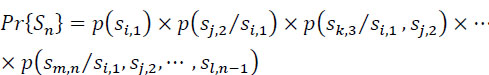
We will use the term discrete source of information Sn to indicate the system selecting, from the set of symbols from As = S, the symbols to transmit:
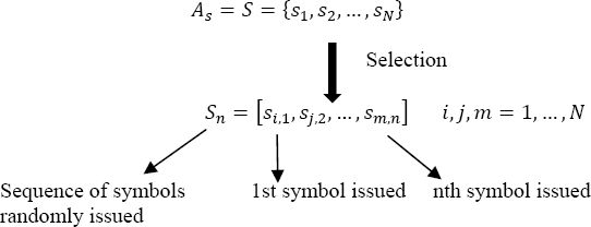
The choice of sm,n is carried out according to a given probability law, which can be steady temporally or variable over time.
2.2. Examples of discrete sources
2.2.1. Simple source (memoryless)
This is a source for which the probability of the occurrence of a symbol does not depend on the previous symbols:
2.2.2. Discrete source with memory
It is a source for which the probability of occurrence of a symbol depends on the symbols already emitted (statistical dependence) and on instants 1, 2, ..., n where they have been emitted:
If the source is in addition stationary then the dependence is only on the ranks and not on the moments when the symbols have been transmitted, so:
that is, the statistical properties are independent of any temporal translation. We can consider that a text written in any language is an example of such a source.
2.2.3. Ergodic source: stationary source with finite memory
The ergodicity of an information source implies that a temporal average calculated over an infinite duration is equal to the statistical average.
2.2.4. First order Markovian source (first order Markov chain)
First order Markov sources play an important role in several domains, for example, in (Caragata et al. 2015), the authors used such a source to model the cryptanalysis of a digital watermarking algorithm.
It is characterized by:
with:
The probability ![]() = pl,k is called transition probability from state l to state k, and:
= pl,k is called transition probability from state l to state k, and:
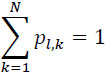
The probability that at time n the source is in the state k is:
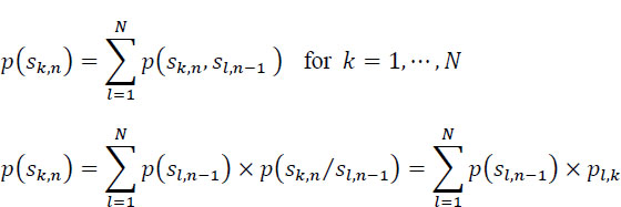
By introducing matrix notations:
Taking into account the relationship [2.8], the relation [2.7] is also written as:
where Tt is the transposed matrix of transition probabilities.
Moreover, if the source is, stationary, then:
in other words, the probabilities of the occurrence of the symbols do not depend on n. It is the same for the transition probabilities pl,k, then the relation [2.9] is written:
where P0 is the matrix of probabilities governing the generation of symbols by the source at the initial instant n = 0.
2.3. Uncertainty, amount of information and entropy (Shannon’s 1948 theorem)
The realization of an event x of probability p(x) conveys a quantity of information h(x) related to its uncertainty. h(x) is an increasing function of its improbability 1/p(x):
If an event x is certain, then p(x) = 1, the uncertainty is zero and therefore the quantity of information h(x) brought by its realization is null.
Moreover, let us consider the realization of a pair of independent events x and y. Their joint realization leads to the amount of information it brings being the sum of the quantities of information brought by each of them:
but ft(x,y) is also written:
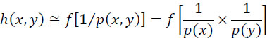
so, from the relationships [2.11] and [2.12], the form of the function f is of logarithmic type, the base a of the logarithmic function can be any ![]()
It is agreed by convention that we select, as the unit of measure of information, the information obtained by the random selection of a single event out of two equally probable events pi = pj = 1/2. In this case, we can write:
If we choose the logarithm in base 2, λ becomes equal to unity and therefore h(xi) = h(xj) = log2(2) = 1 Shannon (Sh) or 1 bit of information, not to be confused with the digital bit (binary digit) which represents one of the binary digits 0 or 1.
Finally, we can then write:
It is sometimes convenient to work with logarithms in base e or with logarithms in base 10. In these cases, the units will be:
loge e = 1 natural unit = 1 nat (we choose 1 among e)
log10 10 = 1 decimal unit = dit (we choose 1 among 10)
Knowing that:
the relationships between the three units are:
- – natural unit: 1 nat = log2(e) = 1/loge(2) = 1.44 bits of information;
- – decimal unit: 1 dit= log2(10) = 1/log10(2) = 3.32 bits of information.
They are pseudo-units without dimension.
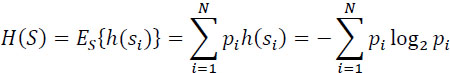
2.3.1. Entropy of a source
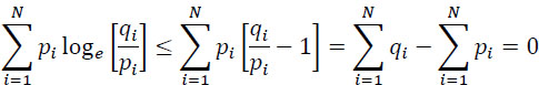
Let a stationary memoryless source S produce random independent events (symbols) s, belonging to a predetermined set [S] = [s1,s2, ... ,sN]. Each event (symbol) Si is of given probability pi, with:

The source S is then characterized by the set of probabilities [P] = [p1,p2, ... ,PN]. We are now interested in the average amount of information from this source of information, that is to say, resulting from the possible set of events (symbols) that it carries out, each is taken into account with its probability of occurrence. This average amount of information from the source S is called “entropy H(S) of the source”.
It is therefore defined by:
2.3.2. Fundamental lemma
Let two probability partitions on S:
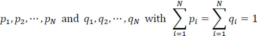
we have the inequality:
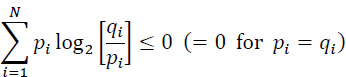
Indeed, since: loge(x) ≤ x − 1, ∀x positive real, then:
2.3.3. Properties of entropy
- – Positive: since 0 ≤ pi ≤ 1;
 (with the agreement
- – Continuous: because it is a sum of continuous functions “log” of each pi.
- – Symmetric: relative to all the variables pi.
- – Upper bounded: entropy has a maximum value:
 got for a uniform law:
- – Additive: let

 , then
2.3.4. Examples of entropy
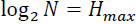
2.3.4.1. Two-event entropy (Bernoulli’s law)
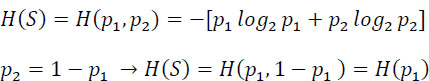
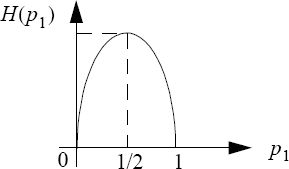
The maximum of the entropy is obtained for ![]() equal to 1 bit of information.
equal to 1 bit of information.
2.3.4.2. Entropy of an alphabetic source with (26 + 1) characters
- – For a uniform law:
⟹H = log2 (27) = 4.75 bits of information per character
- – In the French language (according to a statistical study):
⟹H = 3.98 bits of information per character
Thus, a text of 100 characters provides an information = 398 bits.
The inequality of the probabilities makes a loss of 475 – 398 = 77 bits of information.
2.4. Information rate and redundancy of a source
The information rate of a source is defined by:

Where:
![]() represents the average duration of a symbol emitted by the source.
represents the average duration of a symbol emitted by the source.
The redundancy of a source is defined as follows:
2.5. Discrete channels and entropies
Between the source of information and the destination, there is the medium through which information is transmitted. This medium, including the equipment necessary for transmission, is called the transmission channel (or simply the channel).
Let us consider a discrete stationary and memoryless channel (discrete: the alphabet of the symbols at the input and the one at the output are discrete).
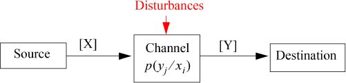
Figure 2.2. Basic transmission system based on a discrete channel. For a color version of this figure, see www.iste.co.uk/assad/digital1.zip
We denote:
- – [X] = [xl, x2, ... , xn]: the set of all the symbols at the input of the channel;
- – [y] = [yi, ... , ym]: the set of all the symbols at the output of the channel;
- – [P(X)] = [p(x1), p(x2), ...,p(xn)]: the vector of probability of symbols at the input of the channel;
- – [P(Y)] = [p(yi), p(y2), ... , p(ym)]: the vector of probability of symbols at the output of the channel.
Because of the perturbations, the space [Y] can be different from the space [X], and the probabilities P(Y) can be different from the probabilities P(X).
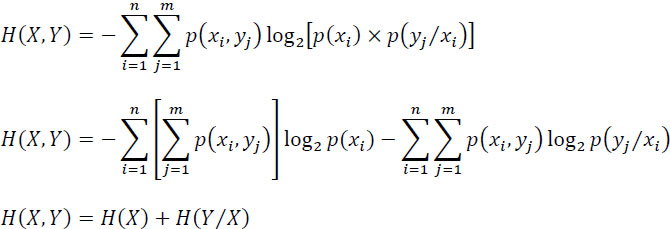
We define a product space [X • Y] and we introduce the matrix of the probabilities of the joint symbols, input-output [P(X, Y)]:
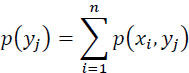
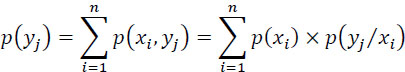
We deduce, from this matrix of probabilities:
We then define the following entropies:
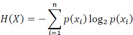
- – the entropy of the source:
[2.23]
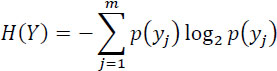
- – the entropy of variable Y at the output of the transmission channel:
[2.24]
- – the entropy of the two joint variables (X, Y)Because of the disturbances in the transmission channel, if the symbolinput-output:
[2.25]

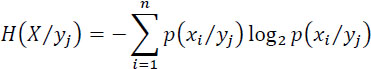
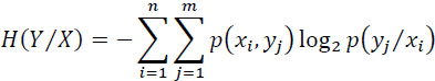
2.5.1. Conditional entropies
Because of the disturbances in the transmission channel, if the symbol yj appears at the output, there is an uncertainty on the symbol xi, j = 1, ... ,,n which has been sent.
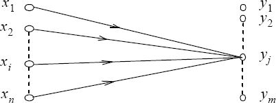
Figure 2.3. Ambiguity on the symbol at the input when yj is received
The average value of this uncertainty, or the entropy associated with the receipt of the symbol yj, is:
The mean value of this entropy for all the possible symbols yj received is:
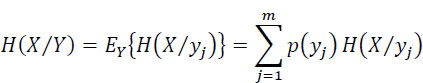
Which can be written as:
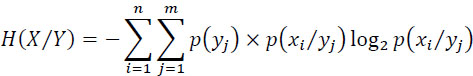
or:
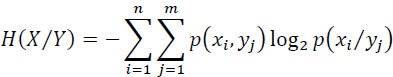
The entropy H(X/Y) is called equivocation (ambiguity) and corresponds to the loss of information due to disturbances (as I(X, Y) = H(X)− H(X/Y)). This will be specified a little further.
Because of disturbances, if the symbol xi is issued, there is uncertainty about the received symbol yj, j = 1, ... , m.
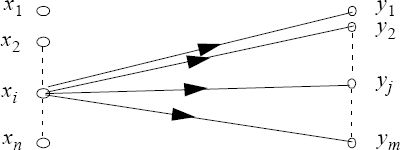
Figure 2.4. Uncertainty on the output when we know the input
The entropy of the random variable Y at the output knowing the X at the input is:
This entropy is a measure of the uncertainty on the output variable when that of the input is known.
The matrix P(Y/X) is called the channel noise matrix:
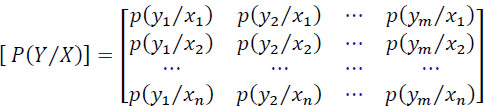
A fundamental property of this matrix is:
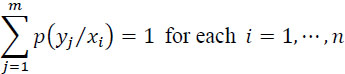
Where: p(yj/xi) is the probability of receiving the symbol yj when the symbol xi has been emitted.
In addition, one has:
with:
p(yj) is the probability of receiving the symbol yjwhatever the symbol xi emitted, and:
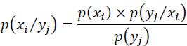
p(xi/yj) is the probability that the symbol xi was issued when the symbol yj is received.
2.5.2. Relations between the various entropies
We can write:
In the same way, as one has: H(Y, X) = H(X, Y), therefore:
In addition, one has the following inequalities:
and similarly:
SPECIAL CASES.–
– Noiseless channel: in this case, on receipt of yj, there is certainty about the symbol actually transmitted, called xi (one-to-one correspondence), therefore:
Consequently:
and:
– Channel with maximum power noise: in this case, the variable at the input is independent of that of the output, i.e.:
We then have:
Note.– In information security, if xi is the plaintext, and yj is the corresponding ciphertext, then p(xi/yi) = p(xi) is the condition of the perfect secret of a cryptosystem.
2.6. Mutual information
The mutual information obtained on the symbol xi when the symbol yj is received is given by:
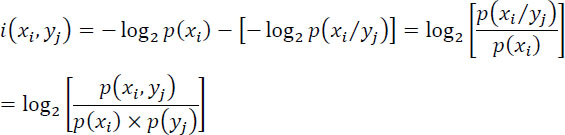
where i(xi, yj) represents the decrease in uncertainty on xi due to the receipt of yj.
The average value of the mutual information, or the amount of information I(X, Y) transmitted through the channel is:
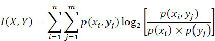
or:
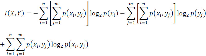
Hence:
Given relationships [2.36] and [2.37], we get:
Special cases.
- – Noiseless channel: X and Y symbols are linked, so:
I(X, Y)=H(X)=H(Y)
- – Channel with maximum power noise: X and Y symbols are independent, therefore:
I(X, Y) = 0
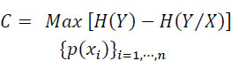
2.7. Capacity, redundancy and efficiency of a discrete channel
Claude Shannon introduced the concept of channel capacity, to measure the efficiency with which information is transmitted, and to find its upper limit.
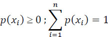
The capacity C of a channel: (information bit/symbol) is the maximum value of the mutual information I(X, Y) over the set of input symbols probabilities ![]()
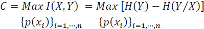
The maximization of I(X, Y) is performed under the constraints that:
The maximum value of I(X, Y)occurs for some well-defined values of these probabilities, which thus define a certain so-called secondary source.
The capacity of the channel can also be related to the unit of time (bitrate Ct of the channel), in this case, one has:

The channel redundancy Rc and the relative channel redundancy pc are defined by:
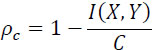
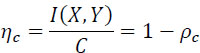
The efficiency of the use of the channel
![]() is defined by
is defined by
2.7.1. Shannon’s theorem: capacity of a communication system
Shannon also formulated the capacity of a communication system by the following relation:
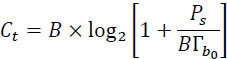
where:
- – B: is the channel bandwidth, in hertz;
- – Ps: is the signal power, in watts;
-
 is the power spectral density of the (supposed) Gaussian and white noise in its frequency band B;
  is the noise power, in watts.
EXAMPLE.– Binary symmetric channel (BSC).
Any binary channel will be characterized by the noise matrix:
If the binary channel is symmetric, then one has:
p(y1/x2) = p(y2/x1) = p
p(y1/x1) = p(y2/x2) = 1 − p
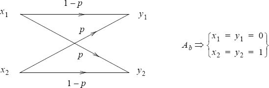
The channel capacity is:
The conditional entropy H(Y/X) is:
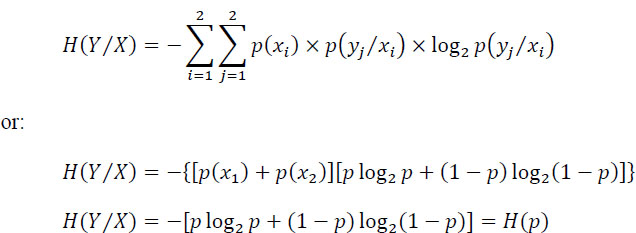
Hence:
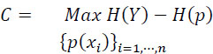
But max H(Y) = 1 for p(y1) = p(y2). It follows from the symmetry of the channel that if p(y1) = p(y2), then p(x1) = p(x2) = 1/2, and C will be given by:
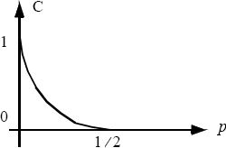
Figure 2.6. Variation of the capacity of a BSC according to p
2.8. Entropies with k random variables
The joined entropy of k random variables is written:
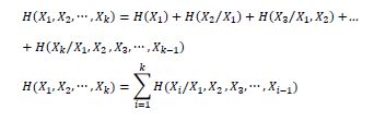
Furthermore, by setting down in the relationship:
One has:
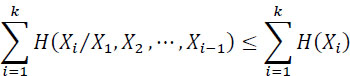
Equality occurs when the variables are independent.