
6
Transmission of an M-ary Digital Signal on a Low-pass Channel
6.1. Introduction
To transmit a digital signal without distortion on a channel (only attenuation α and a given delay τ are accepted), the bandwidth of the transmission medium must be very large compared to the spectrum of the transmitted digital signal. The latter is, in any case, limited to a frequency band Δ/f by filtering the signal at the output of the on-line encoder.
In practice, the bandwidth of the channel is limited. This limitation can come from the transmission medium itself, which can be frequency selective (all the spectral components of the modulated signal do not propagate at the same phase velocity, because of variable attenuation as a function of frequency). This is precisely the case for two-wire and coaxial metal cables, which have a frequency dependent attenuation ![]() .
.
The determining parameters of electric cables with regard to signal transmission are, for a given reference length:
- – frequency transfer function (attenuation and phase shift);
- – characteristic impedance;
- – group propagation delay.
Before tackling the problem of digital transmission, in the next section we present digital systems and standardization for high data rate transmissions.
6.2. Digital systems and standardization for high data rate transmissions
In digital transmission systems, the transmission is actually simultaneous on several information channels. They are characterized by different important features such as:
- – the bitrate in bit/s, which measures the number of binary elements transmitted per unit of time (usually per second);
- – the symbol rate in symbol/s (or modulation speed, in bauds), which measures the number of M-ary symbols transmitted per unit of time;
- – the number of information channels transmitted simultaneously;
- – the structure of the frame, which characterizes the sequential organization of the different channels as well as the auxiliary channels necessary for signaling and locking the frames (frame synchronization);
- – the transmission parameters: the type of transmission medium, the average length of a section, the probability of errors, etc.
For practical reasons, as well as for theoretical and economic reasons, the bitrates found in the digital transmission systems used are not arbitrary but correspond to a digital hierarchy depending on standardization. The digital transmission network, using copper cables as a medium, is based on the use of the so-called “plesiochronous” digital hierarchy (PDH). The word “plesiochronous” comes from the Greek plesio (near) and chronos (time) and reflects the fact that PDH networks use identical but not perfectly synchronized elements: they have the same nominal bitrate for all arteries of the same type, but this bitrate differs slightly depending on the local processing clock. In this hierarchy, there are five types of digital transmission systems: DT1, DT2, DT3, DT4 and DT5, where DTi means “digital transmissions of order i”. It should be noted that a DTi system can transport four DT (i–1) systems simultaneously. The transition from one level to another and vice versa is done by multiplexing and demultiplexing. In addition, transmission systems can be found which transport several hierarchies of the same order simultaneously (for example, n × 34 Mbits or n × 140 Mbits). Note that the bitrates are different in the USA and Japan.
Table 6.1 gives the main features of the five digital transmission systems standardized in Europe.
Table 6.1. Main features of the five digital transmission systems standardized in Europe
| Designation | Bitrate Mbit/s | Related multiplex | Number of telephone channels | Code and frame length | Medium | Nominal length of regeneration |
| DT1 | 2.048 (2) | 30 x 64Kbit/s + 128 Kbit/s | 30/60 channels or 5 channels Conference call or 15 channels Video-conference | HDB3 256 bits (240 useful) | Cable of symmetric pairs ordinaries | 1.8 km |
| DT2 | 8.448 (8) | 4 x DT1 | 120/240 channels or 20 channels Conference call or 60 channels Video-conference | AMI 848 bits = 4 x 212 (824 useful) | Cable of symmetric pairs specials or mini coaxial 0.7/2.9 mm | 4 km ± 400 m |
| DT3 | 34.368 (34) | 4 x DT2 | 480/960 channels or 4 TV channels | – | Cable of coaxial pairs 1.2/4.4 mm | 4 km ± 100 m |
| DT4 | 139.264 (140) | 4 x DT3 | 1,920/3,840 channels or 16 TV channels | 4B3T | Cable of coaxial pairs 1.2/4.4 mm or 2.6/9.5 mm | 2 km ± 50 m |
| DT5 | 564.992 (565) | 4 x DT4 | 7,680/15,360 channels or 64 TV channels | – | Cable of coaxial pairs 2.6/9.5 mm | 1.5 km |
In addition, the flexibility requirements of the transmission network, the necessary improvement in operating and maintenance functions, the appearance of transmissions on optical fibers and the rapid increase in their transmission capacity, the necessary interconnections between networks to high and standardized data rates from different operators have led to the study and standardization of a new synchronous digital hierarchy: SDH (Synchronous Digital Hierarchy).
The use of PDH is most often limited to 140 Mbit/s, after which SDH is preferred.
6.3. Modeling the transmission of an M-ary digital signal through the communication chain
Let us consider the transmission of an M-ary digital signal through a noisy low- pass channel of bandwidth B (see Figure 6.1).
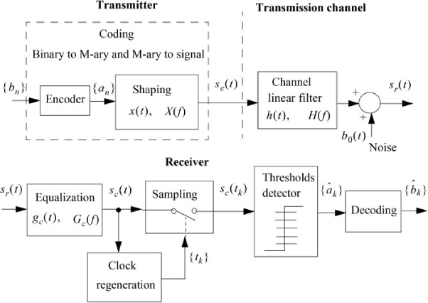
Figure 6.1. Practical chain of a digital baseband communication system
The transmission channel is modeled by a low-pass filter having the following known attenuation, phase shift and delay characteristics:
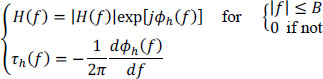
The transmission channel is assumed to be stationary here (its characteristics do not vary over the time) and linear. It only introduces linear distortions on the input signal, since |H(f)| and τh(f) are functions of the frequency.
However, the delay τh(f) is, on the one hand, very negligible compared to the duration of transmission of a symbol (except for very long distance satellite transmissions) and, on the other hand, is taken into account in the choice of the sampling instants. It can therefore not be taken into account directly thereafter.
The noise b0(t) is assumed to be additive at the channel output, and, therefore, at the input of the receiver’s equalization filter. It consists of the sum of the disturbing noise added to the signal during its transmission and the internal noise of the receiver reduced to its input.
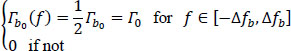
The noise b0(t) is assumed to be 2nd order stationary, Gaussian, centered, of power ![]() independent of the useful signal, and of bilateral power spectral density Γb0(f) constant on a frequency band Δfb (equivalent energy bandwidth) given by:
independent of the useful signal, and of bilateral power spectral density Γb0(f) constant on a frequency band Δfb (equivalent energy bandwidth) given by:
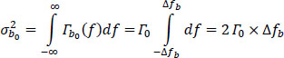
The noise power ![]() is given by:
is given by:
The problem dealt with in this chapter is that of optimizing all the blocks in the transmission chain in order to obtain the best estimate of the symbols {âk}.
The binary sequence {bn} is transformed by the encoder into a sequence {an} where the symbols an are M-ary symmetric symbols:
After filtering by the shaping filter with transfer function X(f) and real impulse response x(t), the digital signal transmitted se(t) is expressed as:
The signal x(t) has an amplitude V and as temporal support the interval [0, θ [ in which θ denotes the period of emission of the symbols, and is not necessarily a rectangular function. In the case where x(t) is a rectangle signal, we then take θ = T for the NRZ code and θ = T/2 for the RZ code.
The signal emitted se(t) is applied to the input of the physical transmission medium (cable) modeled by the low-pass filter with transfer function H(f) and impulse response h(t). The signal sr(t) at the output of the transmission channel (or equivalently at the input of the receiver) is of the form:
where y(t) is the response of the physical transmission medium (cable) to the physical signal x(t) (excluding noise):
and ⊗ is the convolution product.
In the frequency domain, one has:
The input filter at the receiver, also called the “equalization filter”, is intended to compensate for the harmful effects of the transmission medium. Its transfer function is Gc(f) and its impulse response gc(t). It works in a frequency band totally included in the frequency band [–Δfb, Δfb]. It delivers a corrected (also called equalized) signal sc(t):
with:
the response of the equalization filter to signal y(t), that is to say, the response of the whole (cable + equalization) to the elementary pulse x(t), and:
is the result of filtering the noise b0 (t) by the equalization filter. It is characterized by its power spectral density rb1 (f) and its power ![]() .
.
In the frequency domain, one has:
The signal sc (t) is sampled at regularly spaced instants tk of the form:
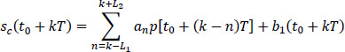
and applied to the input of the decision system. It is then expressed by:
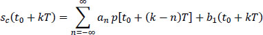
Or, by isolating the term that contains the contribution of the useful symbol ak:
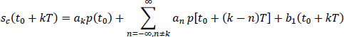
So the signal sc(t0 + kT) is made of the sum of three terms:
- – the useful signal akp(t0) which corresponds to the response of the system (cable + equalization) to the transmission of the elementary symbol ak associated with this time interval;
- – the sum of responses:
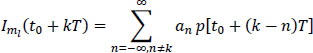
called “intersymbol interference” (ISI). It is a parasitic signal depending on all the symbols interfering with symbol ak transmitted. The latter is the only interesting one over the time interval considered. The set of symbols interfering with the symbol ak defines a message mι belonging to the set M of possible messages of inter-symbol interference. The index mι E M in the relation [6.16] indicates this dependence. The equalization function will aim to maximize the signal p(t0) and cancel (minimize) the ISI;
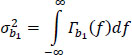
- – the additive noise b1(t0 + kT), stationary, Gaussian, centered, with a power spectral density given by:
and a total power ![]() given by:
given by:
We call Δfc the equivalent energy bandwidth of the equalization filter Gc(f). Since Δfc < Δfb, one then has:
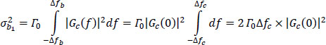
Or again, from [6.3]:
6.3.1. Equivalent energy bandwidth Δfe of a low-pass filter
In practical applications, to facilitate the calculation, it is often interesting to replace a filter G(f) of a very large frequency band (tends towards infinity) by its equivalent Ge(f) (see Figure 6.2), by determining its energy bandwidth Δfe, with the constraint of having the same gain at zero frequency:
|Ge(0)| = |G(0)|
In energy terms, one has:
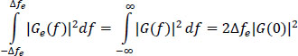
hence:
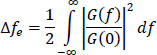
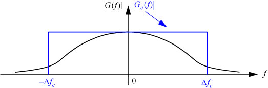
Figure 6.2. Equivalent energy bandwidth Δfe of a low-pass filter. For a color version of this figure, see www.iste.co.uk/assad/digital1.zip
6.4. Characterization of the intersymbol interference: eye pattern
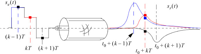
Figure 6.3. Illustration of the intersymbol interference phenomenon. For a color version of this figure, see www.iste.co.uk/assad/digital1.zip
When a signal se (t) made up with a sequence of symbols is applied to a limited-band B transmission channel, one obtains, at the output, a signal sc(t) consisting of the sum of the amplitudes of the individual responses at this time t. The response to each input pulse (here, rectangular and of width T) is, as shown in Figure 6.3, of an elongated bell shape of width λT with λ »1.
A significant widening of the response means that the bandwidth B of the channel is small compared to the symbol rate Ds = 1/T, expressed in symbols/second, of the input signal and vice versa.
The enlargement leads to the overlapping of pulse responses which, consequently, induces the phenomenon of intersymbol interference. The importance of this phenomenon depends on the number and amplitudes of the neighboring pulse responses which are added at the instant tk to the response to the transmitted symbol ak. The effect of ISI can be reduced by increasing the bandwidth of the channel, or by reducing the symbol transmission rate.
6.4.1. Eye pattern
The eye diagram, called this because of its resemblance to the shape of a human eye, is the figure obtained by superimposing all traces or realizations of the signal sc(t) noiseless. It is periodic, of period T.
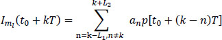
The channel is of limited bandwidth B, let us then suppose that the signal p(t) extends over the interval [–L1T, L1T with L1 and L2 integers, and is zero or negligible outside this interval. Let us examine the set of ISI values contained in the signal sc(t) over the interval [0, T[ for all the realizations of the sequence {an}.
On this interval, the signal sc(t) is expressed (remember that it is assumed to be noise-free):
The possible number of traces of the signal sc(t) is then equal to ML1+L2+1, and 2L1+L2+1 in the case of binary symbols.
The superposition of all these traces constitutes the eye pattern associated with the signal sc(t) on the interval [0, T[. This is, of course, valid for any interval [t1, t1 + T[ where t1is an arbitrary instant.
The eye pattern can be displayed on an oscilloscope. The oscilloscope time base is synchronized to the sampling rate of 1/T frequency, so that at the instants t0 + kT, the spot always occupies the same horizontal position on the screen. If the scanning velocity of the oscilloscope is sufficiently high compared to the persistence of the cathode ray tube or, even better, if the oscilloscope has a trace memory, a large number of traces of sc (t) are visible simultaneously on the screen.
The eye pattern allows direct measurement of the ISI at any time, and, therefore, an assessment of the quality of a transmission link. It shows the importance of the distortion of the digital signal, and allows us to quickly and approximately adjust the equalization function.
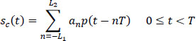
In Figure 6.4 we show all the characteristics that an eye pattern can have in the case of binary symbols. In the general case of M-ary symbols, we will have (M – 1)
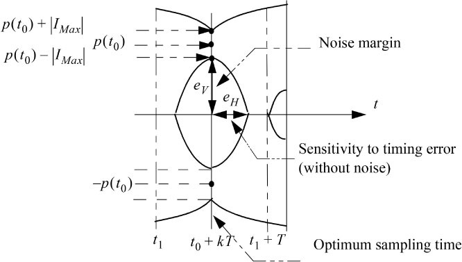
Figure 6.4. Characteristics of the eye diagram: case of binary symbols ak = ± 1
Consider the case where the ISI leads to decision errors in the absence of noise As the optimal decision thresholds without ISI (see formula [6.71]) are distant from 2p(t0), errors due to the ISI may occur if the absolute value of the ISI is greater than p(t0), that is to say:
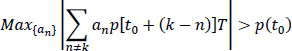
However, the largest absolute value of an is (M – 1), which causes the maximum distortion brought by the ISI to be:
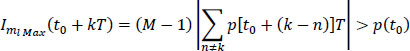
(denoted as |IMax| in Figure 6.4).
When the relation [6.25] is verified, the eye pattern is completely closed at the sampling instants tk, and decision errors are obvious, even in the absence of noise.
The distance ev “vertical half-opening of the eye” represents the amplitude of noise corresponding to the threshold of appearance of the errors. In the absence of noise, it is sufficient that the vertical opening of the eye is greater than zero, so that it is possible to distinguish, without error, the values of two neighboring symbols.
The “horizontal half-opening of the eye” eH represents the maximum tolerable offset of the sampling instant in the absence of noise. In the presence of noise, this tolerance is reduced.
We give two examples of eye diagrams in Figure 6.5: the first (Figure 6.5(a)) concerns the case of binary transmission M= 2, for a signal-to-noise ratio of 15 dB. The second (Figure 6.5(b)) concerns an M-ary transmission with M = 4, for a signal- to-noise ratio of 30 dB.
In both cases, the diagrams are represented for a roll-off factor α = 0.6 (the roll-off factor coefficient will be defined precisely later in the text).
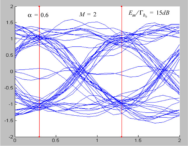
Figure 6.5a. Examples of an eye pattern. For a color version of this figure, see www.iste.co.uk/assad/digital1.zip
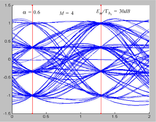
Figure 6.5b. Examples of an eye pattern (following). For a color version of this figure, see www.iste.co.uk/assad/digital1.zip
6.5. Probability of error Pe
Let us first place ourselves in the practical case where the signals p [t0 + (k – n)T] are null or negligible outside the interval [–L1T, L2T].
The expression of the signal obtained after equalization and sampling becomes:
Since (L, + L2 + 1) symbols an contribute to the response sc(t0 + kT), the receiver is likely to receive M(L1+L2+1). different signals, each of duration (L1 + L2 + 1). The decision could be made from M(L1+L2+1) matched filters but its complexity increases exponentially with the number (L1 + L2 + 1).
We are interested in the decision concerning the information symbol ak (of rank k). The signal on which the decision is performed as to the value of the information symbol ak transmitted is:
with:
So one has ML = M(L1+L2) messages m¡ interfering with symbol ak, where:
6.5.1. Probability of error: case of binary symbols ak = ±1
We must first note that when the symbols are binary, then we have T = Tb, where Tb is the duration of a transmitted binary symbol.
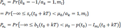
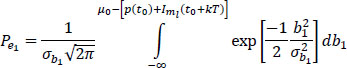
The sample sc(t0 + kT) at the input of the decision system is compared with a single threshold μ0, and a decision âk = d[sc(t0 + kT)] concerning the value of the symbol ak is taken, according to the following rule:
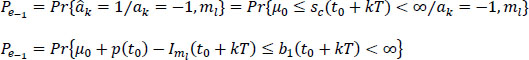
Two types of wrong decision are possible: take the decision âk = 1 knowing that ak = –1, or vice versa.
Hence the two conditional probabilities of wrong decision:
If Pi = Pr{ak = i} with i = [–1,1] is the probability to transmit the symbol ak = i, and pmι = Pr{mι} is the probability to have the interfering message , then, in the case of independent emitted symbols, the probability of error at time tk is expressed by:
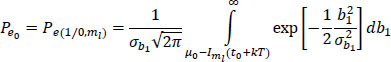
6.5.1.1. Calculation of conditional probabilities of erroneous decision
The signal sample sc(t0 + kT) in the relation [6.27] can then be considered as the realization of a random Gaussian variable of mean value:
and variance:
The reasoning and the calculation which follow are based on the fact that the probability of a random variable can be calculated starting from the knowledge of its density of probability and its support, indeed:

The noise b1 (t0 + kT) is written:
In general, the sample sc (t0 + kT) belongs to an interval [c, d [ depending on the decision thresholds. One can then write:
The decision rule [6.30] is set as follows:
1) One decides that:
hence:
and:
so:
or:
2) In the same way, one decides that:
hence:
and:
so:
or:
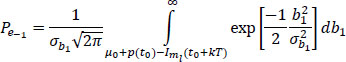
Recall that the probability density of the noise b1 is given by:
and:
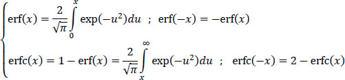
Functions erf(x) and erfc(x) are called the “error function” and the “complementary error function”.
Some authors prefer to use the function Q (x) defined by:
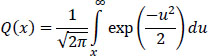
and, in relation with function erfc(x). by:
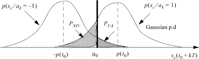
6.5.1.2. Connection with the detection theory
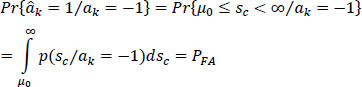
There is a direct connection with the statistical detection theory. Because the false alarm probability PFA (false positive, FP) can be directly deduced with what was previously described:
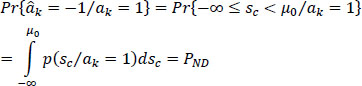
It is the same for the probability of false non detection PND (false negative, FN):
We can then define the two following probabilities:
- – the probability of decision PD:
- – the probability of correct decision Pc:
with:
6.5.1.3. Optimal decision threshold
The optimal decision threshold that minimizes the probability of error Pe is the one that makes null the derivative of Pe with μ0 (Imι(t0 + kT) = 0).
Knowing that:
then:
This leads to the expression of the optimal threshold, denoted μ0opt, given by:
The optimal threshold only depends on the probability distribution {p1, p–1}. For example, if p± > p–1. the threshold moves to negative values, so as to favor the decision âk = 1, that is to say, the most likely a priori binary symbol.
In the case where the binary symbols transmitted are equiprobable, p1 = p–1 = 1/2, then the optimal threshold μ0opt is zero, and the decision system tests only the sign of the sample sc(t0 + kT).
6.5.1.4. Probability of error in the simple case of equiprobability of symbols ak
In this case, one has:
Hence the probability of error Pe:
6.5.2. Probability of error: case of binary RZ code
By adopting the same approach as above, the probability of error for a binary RZ code, according to the relation [6.33], is expressed by:
with:
and:
The optimal threshold is obtained by calculating the threshold value which cancels the derivative of the probability of error in optimal reception:
hence:
In the case of equiprobable symbols, the optimal threshold becomes:
6.5.2.1. Probability of error in the case of equiprobable symbols
In this case:
and then:
6.5.3. Probability of error: general case of M-ary symbols
Let us now consider the general case where the symbols are M-ary and take the following values:
The waveform x(t) is of duration T = kTb. The structure of the receiver remains unchanged. It is composed of a reception filter (impulse response gc(t)) followed by a sampler and a threshold comparator system with (M – 1) thresholds pm. The thresholds pm, in the case of optimal reception and equiprobable symbols, are optimum and located in the center of each interval, delimited by two consecutive values of the sample akp(t0):
with:
where m is a relative integer.
In Figure 6.7 we show the different possible values of the sample akp(t0) and the position of the optimal thresholds.
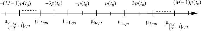
Figure 6.7. Sample values akp(t0) and optimal threshold values (M-ary symbols)
6.5.3.1. Decision rules (symbols ak: âk)
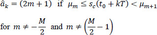
6.5.3.1.1. Case of intermediate values 2m+ 1, where  and m ≠
The decision on symbol ak is carried out by comparing the sample sc(t0 + kT) to the different thresholds μm, and the decision âk = (2m + 1) is taken as soon as sc(t0 + kT) lies between the two consecutive thresholds μm and μm+1:
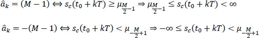
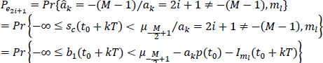
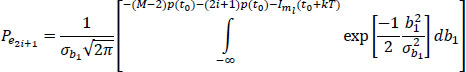
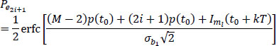
6.5.3.1.2. Case of extreme values +(M - 1)
To decide on extreme values +(M – 1), the sample sc(t0 + kT) is compared to a single threshold in each case:
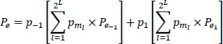
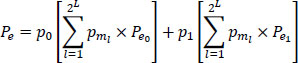
Denoting by p2i+1 the probability of emission of the symbols ak:
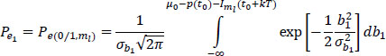
and by Pe2i+1 the conditional probability of error which, conditionally to each value of the symbol ak transmitted and of all the messages m¡ interfering with it, is written:
with:
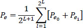
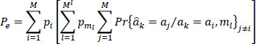
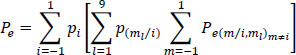
The total average probability of error (wrong decision) is then expressed by:
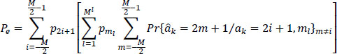
with:
the probability of having the interfering message mι.
The expression [6.78] can be also written as:
In the case where M > 4 and non independent and non equiprobable symbols ak are transmitted, the expression [6.78] of the probability of error is, in general, difficult to calculate analytically. In such cases, the computation is carried out by computer.
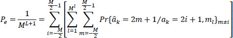
If the symbols ak are independent and equiprobable, then one has:
The expression [6.78] of the error probability becomes:
6.5.3.2. Calculation of the conditional probabilities of error in the case of M-ary symbols (M is even)
Using the decision rule given by the relations [6.73] and [6.74], we can calculate the conditional probabilities of errors Pe2i+1 as follows (we develop the same approach as in the binary case).
In the receiver, the noise at the decision instant is written:
If the signal sc(t0 + kT) at the input of the decision system belongs to the interval [c,d[, consequently the amplitude of the noise b1(t0 + kT) belongs to the following interval:
The decision system operates according to the rules [6.73] and [6.74], so as follows.
6.5.3.2.1. Case of intermediate values of decision
It is decided that:
hence:
then:
Given ak = (2i + 1), the conditional probability of error Pe2i+1 is written:
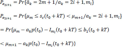
where:
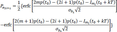
so:
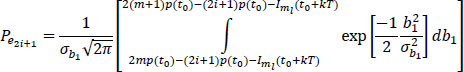
or:
6.5.3.2.2. Case of extreme value of decision âk = (M – 1)
It is decided that:
hence:
then:
with:
Given ak = (2i + 1) Ψ (M – 1), the conditional probability of error Pe2i+1 is written:
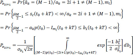
with:
or:
6.5.3.2.3. Case of the extreme value of decision âk = –(M – 1)
It is decided that:
hence:
then:
with:
Given ak = (2i + 1) ≠ –(M – 1), the conditional probability of error Pe2i+1 is written:
with:
or:
This makes it possible to then use the relation [6.78] to calculate the total probability of error.
6.5.4. Probability of error: case of bipolar code
The bipolar code is a code with M = 3 levels such as:
with the two threshold values:
As an example, to calculate the probability of error, we will assume that {bk} are independent but not equiprobable, with:
Given the symbol ak transmitted, the calculation of the conditional probabilities of the different messages of the form mι = (ak–1, ak+1) interfering with symbol ak are given in Tables 6.2, 6.3 and 6.4.
Table 6.2. Calculation of the conditional probabilities P(m[/0) = Pr{mt/ak = 0}
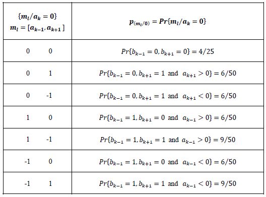
Table 6.3. Calculation of the conditional probabilities p(mι/–1) = Pr{mi/ak = –1}
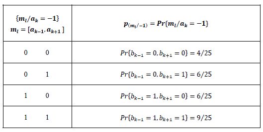
Table 6.4. Calculation of the conditional probabilities p(ml/1 = Pr{ml/ak =1}
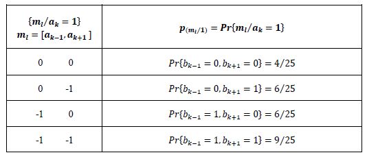
In total, there are nine different messages, of probabilities:
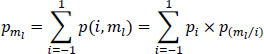
with:

Example.-
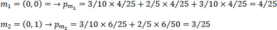
etc.
The probability of error (made of 30 terms) is then:
If only adjacent decision errors are practically possible, i.e.:
then Pe will have only 22 terms.
6.6. Conditions of absence of intersymbol interference: Nyquist criteria
6.6.1. Nyquist temporal criterion
The principle of cancellation of the intersymbol interference implies that, after equalization, at the sampling instants tk = t0 + kT and according to the expression [6.16], the signal p(t) fulfills the following temporal condition:
Taking t0 as time origin, the previous temporal condition becomes (see also Figure 6.8):
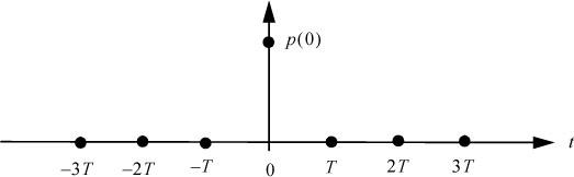
Figure 6.8. Illustration of Nyquist temporal criterion for a null ISI
6.6.2. Nyquist frequency criterion
The pulse p(t) can be of any length and shape, but all of its samples p[(k – n)T] with η ≠ k must be zero. To find the Nyquist frequency criterion, let us look at the transformation of the time condition [6.114] in the frequency domain.
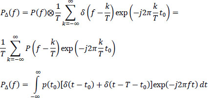
For this, consider the sampled signal ρΔ(t) defined by:
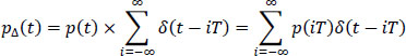
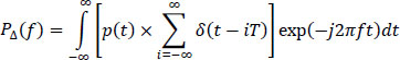
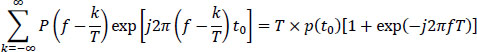
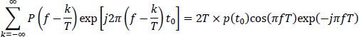
Its Fourier transform PΔ(f) is written:

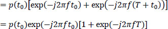
Besides, by the definition of the Fourier transform, we have:
However, the relation [6.115] is also written by using the relation [6.114]:
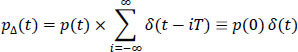
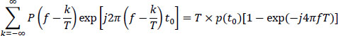
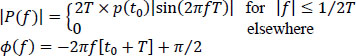
thus:
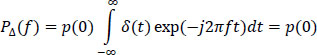
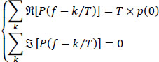
Finally, from [6.116] and [6.119], we deduce the Nyquist frequency criterion:
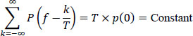
Any function solution of [6.120] fulfills the Nyquist frequency criterion.
6.6.3. Interpretation of the Nyquist frequency criterion
The transmission channel (physical medium) has a bandwidth B. Its transfer function H(f) satisfies:
and, consequently, according to [6.12]:
We can distinguish three cases.
First case
The folded spectrum consists of replicas of P(f) separated by 1/T each other, which do not overlap, and their addition cannot give a constant function (see Figure 6.9). The Nyquist frequency criterion is not verified. This means that we cannot transmit a digital signal with symbol rate Ds (symbol/s) without an ISI in a channel with a bandwidth B < Ds/2.
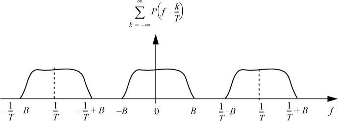
Figure 6.9. Spectrum of 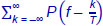 in the case where Ds < 2B
Second case
In this case, the Nyquist criterion is only fulfilled for a given P(f), denoted Nm(f), (see Figures 6.10 and 6.11):
This means that the minimum bandwidth B of the channel required to transmit a digital signal with symbol rate Ds = 1/T and without ISI, is 1/2T, called the
Otherwise, in a channel of width B, one can transmit without ISI a maximum symbol rate of:
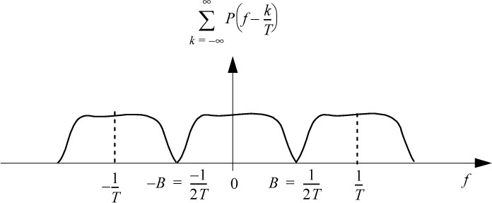
Figure 6.10. Spectrum of  in the case where Ds = 2B
Figure 6.11. First Nyquist frequency criterion
This corresponds to the first Nyquist criterion. It should be noted that the first Nyquist criterion sets a maximum limit at the symbol rate Ds, in symbols per second, and not at the bitrate Db, in bits per second.
Indeed, according to the following relation:
At a given DsMax , the bitrate DbMax can be increased by increasing the number M of levels of the signal. However, the latter is limited by the signal-to-noise ratio.
In the temporal domain, the first Nyquist criterion is translated into the following relation:
This first Nyquist frequency criterion is only of theoretical interest. It has drawbacks which make it unusable in practice, since:
- – the perfectly rectangular template Nm(f) is impractical due to the gain discontinuity at the frequency 1/2T ;
- – function p(t) decreases as 1/|t|, and a small error ɛτ of the sampling instant tk = kT leads to a maximum |IMax| of ISI that is unbounded. Indeed, |IMax| in this case is given, according to [6.25], by:
The arithmetic series of general term 1/|ɛ + m| being divergent, so |Imax| is not bounded, that means that the eye pattern is completely closed at time kT + ɛτ.
Note that taking into account t0, the first Nyquist criterion is expressed in the frequency domain and in the time domain respectively by:
and by:
Third case
The folded spectrum consists of overlapping replicates of P(f) (see Figure 6.12) and it is possible to find many functions P(f) which satisfy the Nyquist frequency criterion called the '“extended Nyquist frequency criterion'” which do not have the drawbacks of the previous solution.
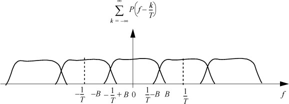
Figure 6.12. Spectrum of 
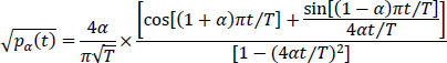
In the case where P(f) = 0 for |f| > 1/T real and positive raised cosine functions are widely used in practice in the transmitter and receiver filters of digital communications systems:
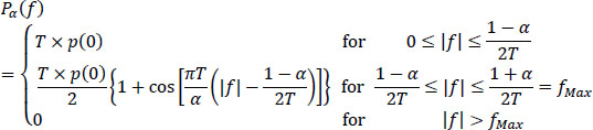
Parameter a, between 0 and 1, is called the “roll-offfactor”. Filters Pα(f) spread 1 + œ over the frequency bandwidth ![]() (by reasoning on the positive frequency domain), that is, an increase of the minimum bandwidth by a factor 1 – α. The impulse response of these filters is of the form:
(by reasoning on the positive frequency domain), that is, an increase of the minimum bandwidth by a factor 1 – α. The impulse response of these filters is of the form:
Figures 6.13 and 6.14 show the normalized and delayed impulse response pα(t) by 5T (so that the filter is causal) and the frequency response Pα(f) for different values of parameter α.
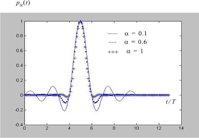
Figure 6.13. Impulse response for different values of the parameter a. For a color version of this figure, see www.iste.co.uk/assad/digital1.zip
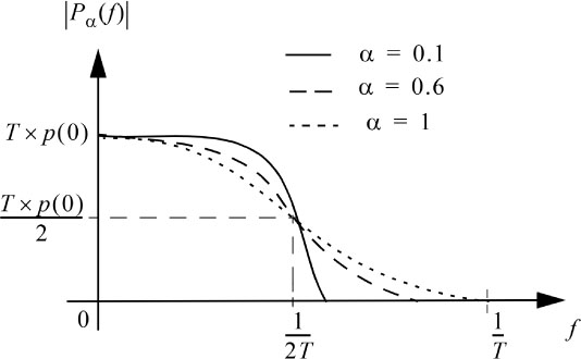
Figure 6.14. Modulus of the frequency response of a raised cosine filter for different values of the parameter α
For α, one gets the rectangular filter Nm(f).
It can be seen that the amplitude of the oscillations of the function pα(t) is smaller as the factor α is large, and therefore the bandwidth of the filter Pα (f) is large. This has an important practical consequence on the sensitivity of the receiver to inaccuracies in the sampling instants. Indeed, an offset ɛτ of the sampling instant will introduce an ISI which is all the more significant as the amplitude of the oscillations is large. At the limit, when a = 1, the amplitude of the oscillations is minimal (decay in 1/t2 of p„(t)), to the point that the function pα(t) is canceled at times (kT + T/2), for k ≠ [0, –1]. The horizontal opening of the eye eH is double compared to the case where α = 0. This improvement comes at the expense of the necessary bandwidth of the channel, twice as much as that of Nyquist ideal.
In Figures 6.15, 6.16, 6.17, and 6.18, we represent the eye pattern in the case of binary symbols an = ±1 for several values of the parameter a. We notice that all the traces of the eye pattern pass through the same points at the sampling times in the absence of noise. We also show, in Figure 6.19, the eye pattern in the case of a quaternary symbol for α = 0.6. Finally, note that the Nyquist filters are not attainable because the function pα(t) is non-causal, pα(t) Ψ 0 for t <0, regardless of the value of the parameter α. However, in practice, the function pα(t) is limited to a support fixed a priori with which we associate a delay line with a half-value delay in order to make causal the function pα(t) as soon as a> 0.1.
These filters are commonly used in digital communications systems with values of a in the order of 0.2 to 0.6.
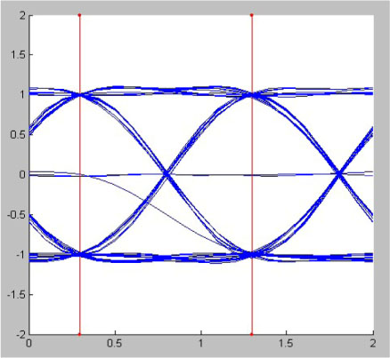
Figure 6.15. Eye pattern (without noise), for α = 1;T = 1 s. For a color

Figure 6.16. Eye pattern (without noise), for α = 0.1; T = 1 s. For a color version of this figure, see www.iste.co.uk/assad/digital1.zip
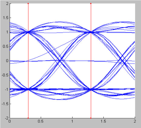
Figure 6.17. Eye pattern (without noise), for α = 0.6; T = 1 s. For a color version of this figure, see www.iste.co.uk/assad/digital1.zip
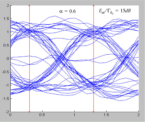
Figure 6.18. Eye pattern (with noise), for α = 0.6 ; Em/Гbo= 15 dB; T = 1 s. For a color version of this figure, see www.iste.co.uk/assad/digital1.zip

Figure 6.19. Eye pattern 4-ary (without noise), for α = 0.6; T = 1 s. For a color version of this figure, see www.iste.co.uk/assad/digital1.zip
NOTE.– The Nyquist frequency criterion also applies when the function P(f) is complex. Condition [6.120] becomes:
Furthermore, in the following, we show that the raised cosine filter which cancels the ISI is distributed between the transmitter and receiver filters. Each impulse response is then given by:
6.7. Optimal distribution of filtering between transmission and reception
The problem dealt with in this section is that of optimizing all the elements of a transmission chain when it is affected by noise.
The cancellation of the ISI at the sampling times requires the equalization performed by the filter Gc(f) to be such that the global transfer function of the transmission chain, see [6.12], satisfies the expanded Nyquist criterion:
where, remember, t0 represents the delay necessary for the emission and reception filters to be causal, and therefore achievable. It also includes the delay brought by the transmission channel.
In fact, in practice, as shown in Figure 6.20, the equalization filter Gc(f) is distributed between the transmitter (transmission filter or preequalization Ge (f)) and the receiver (reception filter or post-equalization Gr(f)). This latter being is called the “equalizer”. Thus, one has:
This distribution makes it possible, among other things, to limit the bandwidth of the signal transmitted so as not to encroach on the adjacent channels. The reception filter limits the spectrum frequency of the received signal and thus eliminates part of the interference due to other channels and reduces the noise power.
It is now a question of finding the optimal filters of emission Ge(f) and reception Gr(f) which maximize the signal-to-noise ratio at the output of the reception filter (that is to say, at the input of the decision-making unit) at the sampling times. The noise b0(t) is considered here as a random, centered, 2nd order stationary Gaussian white process with a constant power spectral density rbo(f), equal to Γ0 in its frequency band and zero elsewhere. The noise b1(t) at the output of the reception filter is expressed by:
It has the same properties as noise b0(t). It power spectral density rb±(f) and power ![]() are given, respectively, by:
are given, respectively, by:
and by:

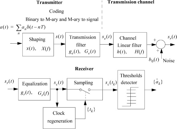
Figure 6.20. Distribution of equalization filtering between transmitter and receiver
In the absence of ISI, the output of the receiver filter at the sampling times t0 + kT is:
The signal sc(t0 + kT) is analogous to that obtained from an infinite bandwidth channel and the M-ary symbols are assumed to be equiprobable, we can show that, under these conditions, the probability of error Pe is given by:
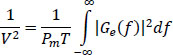
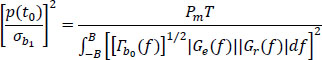
To minimize the probability of error, we have to maximize the signal-to-noise ratio in terms of power:
The amplitude V of the signal at the output of the M-ary to signal encoder is connected to the given average power Pm of the signal sent on the transmission medium.
One has:
and:
The average power Pm is written:
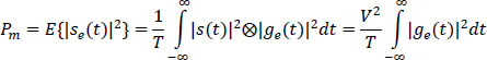
But, also, according to Parseval’s theorem:
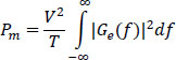
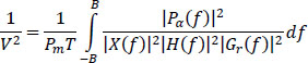
hence:
The filter Ge (f) should fulfill the Nyquist criterion given by [6.134]:
hence:
Maximizing the signal-to-noise ratio means minimizing the noise-to-signal ratio:
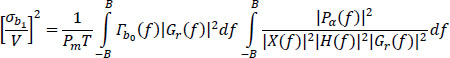
The Cauchy–Schwartz inequality is written:
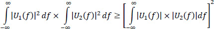
Let:
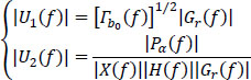
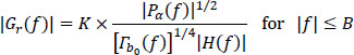
Then the modulus of the reception filter |Gr(/)| (post-equalization filter) tha minimizes the ratio ![]() is given for:
is given for:
where K1 is any real proportionality coefficient
So:
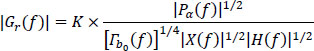
for |f| ≤ B
with ![]()
From [6.147] the modulus of the optimal transmitter filter is expressed by:
In these conditions, the maximum of the signal-to-noise ratio is:
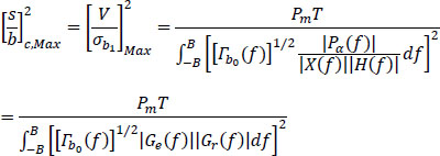
The optimal transmitter and receiver filters are only defined in modules. The phases of the different filters are chosen so as to satisfy the Nyquist criterion [6.134], hence:
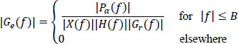
PRACTICAL NOTE.– The preequalization in the transmitter by the optimal emission filter given by relation [6.154] raises practical problems of realization and compatibility between materials of different origins. For this, the principle generally adopted in standardization consists of imposing the characteristics of the signal applied to the transmission medium and leaving maximum freedom for the realization of compatible receivers. For this reason, we define the Nyquist filter Pa(f) and impose the spectrum of the transmitted signal:
The reception filter is then adjusted according to the characteristics |H(f)| of the transmission medium:
Filters | Ge (f)| and |Gr(f)|, thus defined, allow the cancellation of the ISI, but not the maximization of the signal-to-noise ratio at the output of the receiver.
A more efficient but more complex method consists of optimizing the signal-tonoise ratio by applying the condition [6.141] and taking account of the ISI in the estimation process, by carrying out the decision-making using several consecutive samples. An estimate of the sequence of symbols emitted is thus made according to the maximum likelihood a posteriori, that is to say, by determining and maximizing the probability a posteriori that the estimated sequence has been transmitted, knowing the sequence of samples received. This process requires adaptation of the receiver to the characteristics of the transmission channel.
6.7.1. Expression of the minimum probability of error for a low-pass channel satisfying the Nyquist criterion
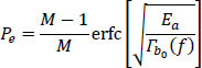
The probability of error of M-ary symbols ak is given by:
This probability of error Pe is minimal when ![]() is maximal. But, according to the expression [6.155], we recall:
is maximal. But, according to the expression [6.155], we recall:
The ratio is maximal if the reception filter is matched to the emission filter:
Moreover, if the noise b0(t) is white noise, then:
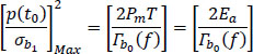
where Ea is the average energy required to transmit a symbol ak .
The probability of error is finally expressed by:
6.8. Transmission with a partial response linear coder
Partial response linear coding introduces, in a controlled manner, an interference between symbols, known to the receiver and therefore able to be taken into account during decoding. The advantage of such coding is that by accepting a certain amount of ISI, it is possible to transmit a signal with a symbol rate Ds = 1/T on a channel having a bandwidth strictly equal to 1/2T.
Two partial response codes characterized by their transfer function are used here to illustrate the result cited above.
The two codes analyzed and evaluated subsequently are:
- – the duobinary code, characterized by its transfer function:
- – the interleaved bipolar code of order 2 whose transfer function is given by:
Figure 6.21 shows the transmission and reception chain with a partial response linear coding. We then adopt the same approach as A. Glavieux and M. Joindot in (Glavieux and Joindot 1996).

Figure 6.21. Transmission and reception chain with partial response linear coding
6.8.1. Transmission using the duobinary code
Let us consider the transmission of a series of binary symbols an over a noisy low-pass channel with bandwidth B. The sample sc(t0 + kT) at the input of the decision block is written in the usual form:
Let us consider that only the symbol ak–1 interferes with the symbol ak, thus producing an ISI equal to ak–1p(t0 + T).
Under these conditions, and assuming that:
The expression of sc(t0 + kT) is then:
The temporal condition of this particular form of ISI is:
The frequency function P(f) that leads to this same ISI should satisfy the following equality:
Or again:
The condition [6.169] is fulfilled by filter P(f):
that satisfies:
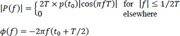
This filter covers a frequency band of 1/2T (by reasoning on the positive frequencies) but, unlike the filter verifying the first Nyquist criterion, it does not present discontinuities at frequencies +1/2T and it is therefore physically achievable (see Figure 6.22, section 6.8.3). Furthermore, the maximum distortion due to an offset ɛ of the optimal sampling instant (t0 + kT) remains finite. The eye pattern is therefore opened in the vicinity of the optimal decision instant. Furthermore, by setting ck = ak + ak–1, the expression [6.166] is written:
NOTE.– The expression [6.172] shows that the transmission of a sequence of independent an binary symbols, in the presence of a particular ISI, is seen as the transmission of a sequence of correlated ternary symbols cn, but without ISI.
6.8.1.1. Demonstration of relation [6.168]
To demonstrate the relationship, we adopt the approach explained in section 6.6. The sampled signal pΔ (t) is written:
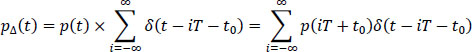
Or considering relations [6.166] and [6.167]:
The respective Fourier transforms of expressions [6.173] and [6.174] are written:
By equalizing the two expressions of pΔ(f), we obtain relation [6.168].
6.8.2. Transmission using 2nd order interleaved bipolar code
In this case, the ISI added to the useful signal at the instant (t0 + kT) is:
–ak–2p(t0 + 2T)
The sample sc(t0 + kT) at the output of the reception filter is equal to:
again, assuming that p(t0 + 2Γ) = p(t0):
To obtain this amount of ISI, the signal p(t) must fulfill the following temporal condition:
By following the same approach as before, we easily show that the function P(f), which leads to the ISI mentioned above, verifies the following relation:
which is fulfilled by a filter P(f) such that:
The modulus | P (f) | of the frequency response is shown in Figure 6.22.
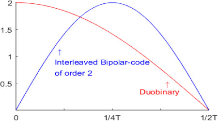
Figure 6.22. Modulus normalized with respect to T × p(t0) of the frequency response |P(f)| of codes duobinary and bipolar interleaved of order 2. For a color version of this figure, see www.iste.co.uk/assad/digital1.zip
As in the case of the duobinary code, the frequency response occupies a frequency band equal to 1/2T (for positive frequencies) and has no discontinuity. In addition, the interleaved bipolar code of order 2 can be used for transmission over a cable, since |P(f)| at f = 0 is zero.
By setting ck = ak – ak–2, the expression [6.178] is written like the expression [6.172]:
and the remark from the previous paragraph concerning the duobinary code applies.
6.8.3. Reception of partial response linear codes
In the previous section, it was shown that the transmission of binary information in the presence of controlled ISI is transformed, thanks to partial response coding, to the transmission of a series of correlated M-ary symbols without ISI.
Recall the relationship between the symbols ck and ak which depends on the type of ISI considered here, namely:
Decoding of binary symbols ![]() is obtained directly from the symbols ck without propagation of error, thanks to the function of precoding on transmission.
is obtained directly from the symbols ck without propagation of error, thanks to the function of precoding on transmission.
6.8.3.1. Case of duobinary coding
The precoder generates a sequence ![]() such as:
such as:
The transcoder generates, at output, a symmetrical binary sequence {ak}:
such that it generates:
The relation defining the operation of the partial response coder is expressed by:
with ck ∈ [0, ±2].
Then, according to [6.187], we can write:
then:
So a direct estimate of the transmitted binary sequence ![]() from the estimated sequence of symbols
from the estimated sequence of symbols ![]() received is:
received is:
6.8.3.2. Example of duobinary coding and decoding
In Figure 6.23, we give an example of duobinary coding and decoding.
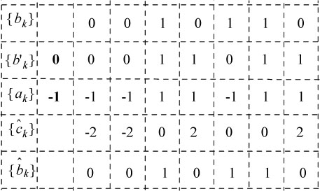
Figure 6.23. Example of duobinary coding and decoding
We can easily see that the absence of precoding on transmission would lead to a propagation of decision errors on the binary symbols {bk}. Indeed, in this case, according to [6.187], by replacing ![]() by bk, one has:
by bk, one has:
So, if the binary element bk–1 is badly decoded, the binary element bk will also almost certainly be.
6.8.3.3. Case of 2nd order interleaved bipolar coding
In this case, the precoder is defined by the following rule:
The transcoding operation is the same whatever the code used, and it is therefore governed by relation [6.185].
The relation defining the operation of the partial response coder is written:
with ck ∈ [0, ±2].
Hence:
This relation shows the instantaneous estimate of the sequence ![]() sent from the sequence
sent from the sequence ![]() received:
received:
EXAMPLE.– 2nd order interleaved bipolar coding and decoding.
Figure 6.24 gives an example of 2nd order interleaved bipolar coding and decoding.
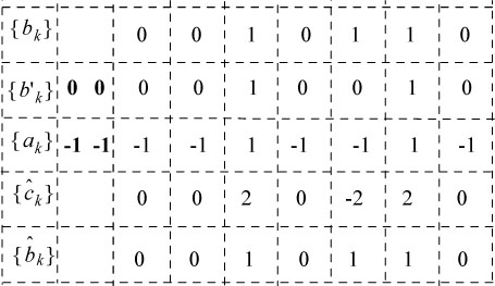
Figure 6.24. Example of 2nd order interleaved bipolar coding and decoding
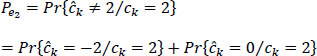
6.8.4. Probability of error Pe
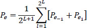
Insofar as the binary elements bk are independent and equiprobable on the alphabet {0,1}, the symbols ck take the values {–2,0,2} with, respectively, the following probabilities: ļi, 2,.
The probability of error is then equal to:
where Pek is the conditional probability that ck = k with k = {–2,0,2}.
Let:
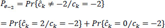
and:
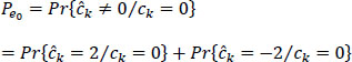
By comparing the sample sc(t0 + kT) to a pair of thresholds –p(t0) and p(t0), we can easily calculate the different expressions of conditional probabilities.
6.8.4.1. Calculation of conditional probabilities
This now classic calculation is thus developed (see also Figure 6.25):
if:
where:
so:
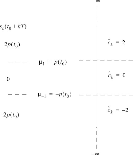
Figure 6.25. Sample values, optimal thresholds and estimation classes 
Application of the decision rules
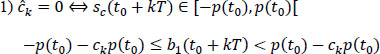
hence:
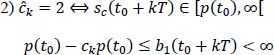
hence:
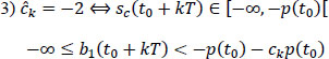
hence:
NOTE.– As soon as the signal-to-noise ratio Emb/Γb0 is sufficiently large, one can make the reasonable assumption of neglecting the possibility of decoding ![]() when ck =2 or vice versa. The probability of error on the binary digit Peb is equal to the probability of error Pe on the symbols c.
when ck =2 or vice versa. The probability of error on the binary digit Peb is equal to the probability of error Pe on the symbols c.