6
Architecture
6.6 Lights, Camera, Action: Compiling, Assembling, and Loading

6.1 Introduction
The previous chapters introduced digital design principles and building blocks. In this chapter, we jump up a few levels of abstraction to define the architecture of a computer. The architecture is the programmer’s view of a computer. It is defined by the instruction set (language) and operand locations (registers and memory). Many different architectures exist, such as x86, MIPS, SPARC, and PowerPC.
The first step in understanding any computer architecture is to learn its language. The words in a computer’s language are called instructions. The computer’s vocabulary is called the instruction set. All programs running on a computer use the same instruction set. Even complex software applications, such as word processing and spreadsheet applications, are eventually compiled into a series of simple instructions such as add, subtract, and jump. Computer instructions indicate both the operation to perform and the operands to use. The operands may come from memory, from registers, or from the instruction itself.
Computer hardware understands only 1’s and 0’s, so instructions are encoded as binary numbers in a format called machine language. Just as we use letters to encode human language, computers use binary numbers to encode machine language. Microprocessors are digital systems that read and execute machine language instructions. However, humans consider reading machine language to be tedious, so we prefer to represent the instructions in a symbolic format called assembly language.
The instruction sets of different architectures are more like different dialects than different languages. Almost all architectures define basic instructions, such as add, subtract, and jump, that operate on memory or registers. Once you have learned one instruction set, understanding others is fairly straightforward.
What is the best architecture to study when first learning the subject?
Commercially successful architectures such as x86 are satisfying to study because you can use them to write programs on real computers. Unfortunately, many of these architectures are full of warts and idiosyncrasies accumulated over years of haphazard development by different engineering teams, making the architectures difficult to understand and implement.
Many textbooks teach imaginary architectures that are simplified to illustrate the key concepts.
We follow the lead of David Patterson and John Hennessy in their text Computer Organization and Design by focusing on the MIPS architecture. Hundreds of millions of MIPS microprocessors have shipped, so the architecture is commercially very important. Yet it is a clean architecture with little odd behavior. At the end of this chapter, we briefly visit the x86 architecture to compare and contrast it with MIPS.
A computer architecture does not define the underlying hardware implementation. Often, many different hardware implementations of a single architecture exist. For example, Intel and Advanced Micro Devices (AMD) both sell various microprocessors belonging to the same x86 architecture. They all can run the same programs, but they use different underlying hardware and therefore offer trade-offs in performance, price, and power. Some microprocessors are optimized for high-performance servers, whereas others are optimized for long battery life in laptop computers. The specific arrangement of registers, memories, ALUs, and other building blocks to form a microprocessor is called the microarchitecture and will be the subject of Chapter 7. Often, many different microarchitectures exist for a single architecture.
In this text, we introduce the MIPS architecture that was first developed by John Hennessy and his colleagues at Stanford in the 1980s. MIPS processors are used by, among others, Silicon Graphics, Nintendo, and Cisco. We start by introducing the basic instructions, operand locations, and machine language formats. We then introduce more instructions used in common programming constructs, such as branches, loops, array manipulations, and function calls.
Throughout the chapter, we motivate the design of the MIPS architecture using four principles articulated by Patterson and Hennessy: (1) simplicity favors regularity; (2) make the common case fast; (3) smaller is faster; and (4) good design demands good compromises.
6.2 Assembly Language
Assembly language is the human-readable representation of the computer’s native language. Each assembly language instruction specifies both the operation to perform and the operands on which to operate. We introduce simple arithmetic instructions and show how these operations are written in assembly language. We then define the MIPS instruction operands: registers, memory, and constants.
This chapter assumes that you already have some familiarity with a high-level programming language such as C, C++, or Java. (These languages are practically identical for most of the examples in this chapter, but where they differ, we will use C.) Appendix C provides an introduction to C for those with little or no prior programming experience.
6.2.1 Instructions
The most common operation computers perform is addition. Code Example 6.1 shows code for adding variables b and c and writing the result to a. The code is shown on the left in a high-level language (using the syntax of C, C++, and Java), and then rewritten on the right in MIPS assembly language. Note that statements in a C program end with a semicolon.
Code Example 6.1 Addition
High-Level Code
a = b + c;
MIPS Assembly Code
add a, b, c
Code Example 6.2 Subtraction
High-Level Code
a = b − c;
MIPS Assembly Code
sub a, b, c
The first part of the assembly instruction, add, is called the mnemonic and indicates what operation to perform. The operation is performed on b and c, the source operands, and the result is written to a, the destination operand.
Code Example 6.2 shows that subtraction is similar to addition. The instruction format is the same as the add instruction except for the operation specification, sub. This consistent instruction format is an example of the first design principle:
Design Principle 1: Simplicity favors regularity.
mnemonic (pronounced ni-mon-ik) comes from the Greek word μιμνΕσκεστηαι, to remember. The assembly language mnemonic is easier to remember than a machine language pattern of 0’s and 1’s representing the same operation.
Instructions with a consistent number of operands—in this case, two sources and one destination—are easier to encode and handle in hardware. More complex high-level code translates into multiple MIPS instructions, as shown in Code Example 6.3.
In the high-level language examples, single-line comments begin with // and continue until the end of the line. Multiline comments begin with /* and end with */. In assembly language, only single-line comments are used. They begin with # and continue until the end of the line. The assembly language program in Code Example 6.3 requires a temporary variable t to store the intermediate result. Using multiple assembly language instructions to perform more complex operations is an example of the second design principle of computer architecture:
Design Principle 2: Make the common case fast.
Code Example 6.3 More Complex Code
High-Level Code
a = b + c − d; // single-line comment
/* multiple-line
comment */
MIPS Assembly Code
sub t, c, d # t = c − d
add a, b, t # a = b + t
The MIPS instruction set makes the common case fast by including only simple, commonly used instructions. The number of instructions is kept small so that the hardware required to decode the instruction and its operands can be simple, small, and fast. More elaborate operations that are less common are performed using sequences of multiple simple instructions. Thus, MIPS is a reduced instruction set computer (RISC) architecture. Architectures with many complex instructions, such as Intel’s x86 architecture, are complex instruction set computers (CISC). For example, x86 defines a “string move” instruction that copies a string (a series of characters) from one part of memory to another. Such an operation requires many, possibly even hundreds, of simple instructions in a RISC machine. However, the cost of implementing complex instructions in a CISC architecture is added hardware and overhead that slows down the simple instructions.
A RISC architecture minimizes the hardware complexity and the necessary instruction encoding by keeping the set of distinct instructions small. For example, an instruction set with 64 simple instructions would need log264 = 6 bits to encode the operation. An instruction set with 256 complex instructions would need log2256 = 8 bits of encoding per instruction. In a CISC machine, even though the complex instructions may be used only rarely, they add overhead to all instructions, even the simple ones.
6.2.2 Operands: Registers, Memory, and Constants
An instruction operates on operands. In Code Example 6.1 the variables a, b, and c are all operands. But computers operate on 1’s and 0’s, not variable names. The instructions need a physical location from which to retrieve the binary data. Operands can be stored in registers or memory, or they may be constants stored in the instruction itself. Computers use various locations to hold operands in order to optimize for speed and data capacity. Operands stored as constants or in registers are accessed quickly, but they hold only a small amount of data. Additional data must be accessed from memory, which is large but slow. MIPS is called a 32-bit architecture because it operates on 32-bit data. (The MIPS architecture has been extended to 64 bits in commercial products, but we will consider only the 32-bit form in this book.)
Registers
Instructions need to access operands quickly so that they can run fast. But operands stored in memory take a long time to retrieve. Therefore, most architectures specify a small number of registers that hold commonly used operands. The MIPS architecture uses 32 registers, called the register set or register file. The fewer the registers, the faster they can be accessed. This leads to the third design principle:
Design Principle 3: Smaller is faster.
Looking up information from a small number of relevant books on your desk is a lot faster than searching for the information in the stacks at a library. Likewise, reading data from a small set of registers (for example, 32) is faster than reading it from 1000 registers or a large memory. A small register file is typically built from a small SRAM array (see Section 5.5.3). The SRAM array uses a small decoder and bitlines connected to relatively few memory cells, so it has a shorter critical path than a large memory does.
Code Example 6.4 shows the add instruction with register operands. MIPS register names are preceded by the $ sign. The variables a, b, and c are arbitrarily placed in $s0, $s1, and $s2. The name $s1 is pronounced “register s1” or “dollar s1”. The instruction adds the 32-bit values contained in $s1 (b) and $s2 (c) and writes the 32-bit result to $s0 (a).
MIPS generally stores variables in 18 of the 32 registers: $s0–$s7, and $t0–$t9. Register names beginning with $s are called saved registers. Following MIPS convention, these registers store variables such as a, b, and c. Saved registers have special connotations when they are used with function calls (see Section 6.4.6). Register names beginning with $t are called temporary registers. They are used for storing temporary variables. Code Example 6.5 shows MIPS assembly code using a temporary register, $t0, to store the intermediate calculation of c – d.
Code Example 6.4 Register Operands
High-Level Code
a = b + c;
MIPS Assembly Code
# $s0 = a, $s1 = b, $s2 = c
add $s0, $s1, $s2 # a = b + c
Code Example 6.5 Temporary Registers
High-Level Code
a = b + c − d;
MIPS Assembly Code
# $s0 = a, $s1 = b, $s2 = c, $s3 = d
sub $t0, $s2, $s3 # t = c − d
add $s0, $s1, $t0 # a = b + t
Example 6.1 Translating High-Level Code to Assembly Language
Translate the following high-level code into assembly language. Assume variables a–c are held in registers $s0–$s2 and f–j are in $s3–$s7.
a = b – c;
f = (g + h) − (i + j);
Solution
The program uses four assembly language instructions.
# MIPS assembly code
# $s0 = a, $s1 = b, $s2 = c, $s3 = f, $s4 = g, $s5 = h
# $s6 = i, $s7 = j
sub $s0, $s1, $s2 # a = b – c
add $t0, $s4, $s5 # $t0 = g + h
add $t1, $s6, $s7 # $t1 = i + j
sub $s3, $t0, $t1 # f = (g + h) – (i + j)
The Register Set
The MIPS architecture defines 32 registers. Each register has a name and a number ranging from 0 to 31. Table 6.1 lists the name, number, and use for each register. $0 always contains the value 0 because this constant is so frequently used in computer programs. We have also discussed the $s and $t registers. The remaining registers will be described throughout this chapter.
Table 6.1 MIPS register set
| Name | Number | Use |
| $0 | 0 | the constant value 0 |
| $at | 1 | assembler temporary |
| $v0–$v1 | 2–3 | function return value |
| $a0–$a3 | 4–7 | function arguments |
| $t0–$t7 | 8–15 | temporary variables |
| $s0–$s7 | 16–23 | saved variables |
| $t8–$t9 | 24–25 | temporary variables |
| $k0–$k1 | 26–27 | operating system (OS) temporaries |
| $gp | 28 | global pointer |
| $sp | 29 | stack pointer |
| $fp | 30 | frame pointer |
| $ra | 31 | function return address |
Memory
If registers were the only storage space for operands, we would be confined to simple programs with no more than 32 variables. However, data can also be stored in memory. When compared to the register file, memory has many data locations, but accessing it takes a longer amount of time. Whereas the register file is small and fast, memory is large and slow. For this reason, commonly used variables are kept in registers. By using a combination of memory and registers, a program can access a large amount of data fairly quickly. As described in Section 5.5, memories are organized as an array of data words. The MIPS architecture uses 32-bit memory addresses and 32-bit data words.
MIPS uses a byte-addressable memory. That is, each byte in memory has a unique address. However, for explanation purposes only, we first introduce a word-addressable memory, and afterward describe the MIPS byte-addressable memory.
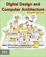
Figure 6.1 shows a memory array that is word-addressable. That is, each 32-bit data word has a unique 32-bit address. Both the 32-bit word address and the 32-bit data value are written in hexadecimal in Figure 6.1. For example, data 0xF2F1AC07 is stored at memory address 1. Hexadecimal constants are written with the prefix 0x. By convention, memory is drawn with low memory addresses toward the bottom and high memory addresses toward the top.
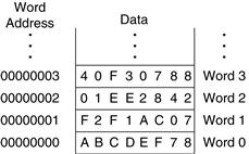
Figure 6.1 Word-addressable memory
MIPS uses the load word instruction, lw, to read a data word from memory into a register. Code Example 6.6 loads memory word 1 into $s3.
The lw instruction specifies the effective address in memory as the sum of a base address and an offset. The base address (written in parentheses in the instruction) is a register. The offset is a constant (written before the parentheses). In Code Example 6.6, the base address is $0, which holds the value 0, and the offset is 1, so the lw instruction reads from memory address ($0 + 1) = 1. After the load word instruction (lw) is executed, $s3 holds the value 0xF2F1AC07, which is the data value stored at memory address 1 in Figure 6.1.
Code Example 6.6 Reading Word-Addressable Memory
Assembly Code
# This assembly code (unlike MIPS) assumes word-addressable memory
lw $s3, 1($0) # read memory word 1 into $s3
Code Example 6.7 Writing Word-Addressable Memory
Assembly Code
# This assembly code (unlike MIPS) assumes word-addressable memory
sw $s7, 5($0) # write $s7 to memory word 5
Similarly, MIPS uses the store word instruction, sw, to write a data word from a register into memory. Code Example 6.7 writes the contents of register $s7 into memory word 5. These examples have used $0 as the base address for simplicity, but remember that any register can be used to supply the base address.
The previous two code examples have shown a computer architecture with a word-addressable memory. The MIPS memory model, however, is byte-addressable, not word-addressable. Each data byte has a unique address. A 32-bit word consists of four 8-bit bytes. So each word address is a multiple of 4, as shown in Figure 6.2. Again, both the 32-bit word address and the data value are given in hexadecimal.
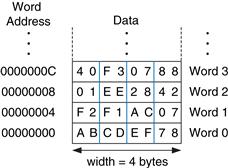
Figure 6.2 Byte-addressable memory
Code Example 6.8 shows how to read and write words in the MIPS byte-addressable memory. The word address is four times the word number. The MIPS assembly code reads words 0, 2, and 3 and writes words 1, 8, and 100. The offset can be written in decimal or hexadecimal.
The MIPS architecture also provides the lb and sb instructions that load and store single bytes in memory rather than words. They are similar to lw and sw and will be discussed further in Section 6.4.5.
Byte-addressable memories are organized in a big-endian or little-endian fashion, as shown in Figure 6.3. In both formats, the most significant byte (MSB) is on the left and the least significant byte (LSB) is on the right. In big-endian machines, bytes are numbered starting with 0 at the big (most significant) end. In little-endian machines, bytes are numbered starting with 0 at the little (least significant) end. Word addresses are the same in both formats and refer to the same four bytes. Only the addresses of bytes within a word differ.
Code Example 6.8 Accessing Byte-Addressable Memory
MIPS Assembly Code
lw $s0, 0($0) # read data word 0 (0xABCDEF78) into $s0
lw $s1, 8($0) # read data word 2 (0x01EE2842) into $s1
lw $s2, OxC($0) # read data word 3 (0x40F30788) into $s2
sw $s3, 4($0) # write $s3 to data word 1
sw $s4, 0x20($0) # write $s4 to data word 8
sw $s5, 400($0) # write $s5 to data word 100

Figure 6.3 Big- and little-endian memory addressing
Example 6.2 Big- and Little-Endian Memory
Suppose that $s0 initially contains 0x23456789. After the following program is run on a big-endian system, what value does $s0 contain? In a little-endian system? lb $s0, 1($0) loads the data at byte address (1 + $0) = 1 into the least significant byte of $s0. lb is discussed in detail in Section 6.4.5.
sw $s0, 0($0)
lb $s0, 1($0)
Solution
Figure 6.4 shows how big- and little-endian machines store the value 0x23456789 in memory word 0. After the load byte instruction, lb $s0, 1($0), $s0 would contain 0x00000045 on a big-endian system and 0x00000067 on a little-endian system.
Figure 6.4 Big-endian and little-endian data storage
IBM’s PowerPC (formerly found in Macintosh computers) uses big-endian addressing. Intel’s x86 architecture (found in PCs) uses little-endian addressing. Some MIPS processors are little-endian, and some are big-endian.1 The choice of endianness is completely arbitrary but leads to hassles when sharing data between big-endian and little-endian computers. In examples in this text, we will use little-endian format whenever byte ordering matters.

The terms big-endian and little-endian come from Jonathan Swift’s Gulliver’s Travels, first published in 1726 under the pseudonym of Isaac Bickerstaff. In his stories the Lilliputian king required his citizens (the Little-Endians) to break their eggs on the little end. The Big-Endians were rebels who broke their eggs on the big end.
The terms were first applied to computer architectures by Danny Cohen in his paper “On Holy Wars and a Plea for Peace” published on April Fools Day, 1980 (USC/ISI IEN 137). (Photo courtesy of The Brotherton Collection, IEEDS University Library.)
In the MIPS architecture, word addresses for lw and sw must be word aligned. That is, the address must be divisible by 4. Thus, the instruction lw $s0, 7($0) is an illegal instruction. Some architectures, such as x86, allow non-word-aligned data reads and writes, but MIPS requires strict alignment for simplicity. Of course, byte addresses for load byte and store byte, lb and sb, need not be word aligned.
Constants/Immediates
Load word and store word, lw and sw, also illustrate the use of constants in MIPS instructions. These constants are called immediates, because their values are immediately available from the instruction and do not require a register or memory access. Add immediate, addi, is another common MIPS instruction that uses an immediate operand. addi adds the immediate specified in the instruction to a value in a register, as shown in Code Example 6.9.
Code Example 6.9 Immediate Operands
High-Level Code
a = a + 4;
b = a − 12;
MIPS Assembly Code
# $s0 = a, $s1 = b
addi $s0, $s0, 4 # a = a + 4
addi $s1, $s0, −12 # b = a − 12
The immediate specified in an instruction is a 16-bit two’s complement number in the range [–32,768, 32,767]. Subtraction is equivalent to adding a negative number, so, in the interest of simplicity, there is no subi instruction in the MIPS architecture.
Recall that the add and sub instructions use three register operands. But the lw, sw, and addi instructions use two register operands and a constant. Because the instruction formats differ, lw and sw instructions violate design principle 1: simplicity favors regularity. However, this issue allows us to introduce the last design principle:
Design Principle 4: Good design demands good compromises.
A single instruction format would be simple but not flexible. The MIPS instruction set makes the compromise of supporting three instruction formats. One format, used for instructions such as add and sub, has three register operands. Another, used for instructions such as lw and addi, has two register operands and a 16-bit immediate. A third, to be discussed later, has a 26-bit immediate and no registers. The next section discusses the three MIPS instruction formats and shows how they are encoded into binary.
6.3 Machine Language
Assembly language is convenient for humans to read. However, digital circuits understand only 1’s and 0’s. Therefore, a program written in assembly language is translated from mnemonics to a representation using only 1’s and 0’s called machine language.
MIPS uses 32-bit instructions. Again, simplicity favors regularity, and the most regular choice is to encode all instructions as words that can be stored in memory. Even though some instructions may not require all 32 bits of encoding, variable-length instructions would add too much complexity. Simplicity would also encourage a single instruction format, but, as already mentioned, that is too restrictive. MIPS makes the compromise of defining three instruction formats: R-type, I-type, and J-type. This small number of formats allows for some regularity among all the types, and thus simpler hardware, while also accommodating different instruction needs, such as the need to encode large constants in the instruction. R-type instructions operate on three registers. I-type instructions operate on two registers and a 16-bit immediate. J-type (jump) instructions operate on one 26-bit immediate. We introduce all three formats in this section but leave the discussion of J-type instructions for Section 6.4.2.
6.3.1 R-Type Instructions
The name R-type is short for register-type. R-type instructions use three registers as operands: two as sources, and one as a destination. Figure 6.5 shows the R-type machine instruction format. The 32-bit instruction has six fields: op, rs, rt, rd, shamt, and funct. Each field is five or six bits, as indicated.

Figure 6.5 R-type machine instruction format
The operation the instruction performs is encoded in the two fields highlighted in blue: op (also called opcode or operation code) and funct (also called the function). All R-type instructions have an opcode of 0. The specific R-type operation is determined by the funct field. For example, the opcode and funct fields for the add instruction are 0 (0000002) and 32 (1000002), respectively. Similarly, the sub instruction has an opcode and funct field of 0 and 34.
The operands are encoded in the three fields: rs, rt, and rd. The first two registers, rs and rt, are the source registers; rd is the destination register. The fields contain the register numbers that were given in Table 6.1. For example, $s0 is register 16.
rs is short for “register source.” rt comes after rs alphabetically and usually indicates the second register source.
The fifth field, shamt, is used only in shift operations. In those instructions, the binary value stored in the 5-bit shamt field indicates the amount to shift. For all other R-type instructions, shamt is 0.
Figure 6.6 shows the machine code for the R-type instructions add and sub. Notice that the destination is the first register in an assembly language instruction, but it is the third register field (rd) in the machine language instruction. For example, the assembly instruction add $s0, $s1, $s2 has rs = $s1 (17), rt = $s2 (18), and rd = $s0 (16).
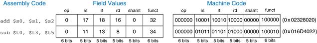
Figure 6.6 Machine code for R-type instructions
For MIPS instructions used in this book, Tables B.1 and B.2 in Appendix B define the opcode values for all instructions and the funct field values for R-type instructions.
Example 6.3 Translating Assembly Language to Machine Language
Translate the following assembly language statement into machine language.
add $t0, $s4, $s5
Solution
According to Table 6.1, $t0, $s4, and $s5 are registers 8, 20, and 21. According to Tables B.1 and B.2, add has an opcode of 0 and a funct code of 32. Thus, the fields and machine code are given in Figure 6.7. The easiest way to write the machine language in hexadecimal is to first write it in binary, then look at consecutive groups of four bits, which correspond to hexadecimal digits (indicated in blue). Hence, the machine language instruction is 0x02954020.

Figure 6.7 Machine code for the R-type instruction of Example 6.3
6.3.2 l-Type Instructions
The name I-type is short for immediate-type. I-type instructions use two register operands and one immediate operand. Figure 6.8 shows the I-type machine instruction format. The 32-bit instruction has four fields: op, rs, rt, and imm. The first three fields, op, rs, and rt, are like those of R-type instructions. The imm field holds the 16-bit immediate.
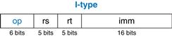
Figure 6.8 I-type instruction format
The operation is determined solely by the opcode, highlighted in blue. The operands are specified in the three fields rs, rt, and imm. rs and imm are always used as source operands. rt is used as a destination for some instructions (such as addi and lw) but as another source for others (such as sw).
Figure 6.9 shows several examples of encoding I-type instructions. Recall that negative immediate values are represented using 16-bit two’s complement notation. rt is listed first in the assembly language instruction when it is used as a destination, but it is the second register field in the machine language instruction.
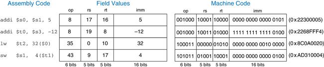
Figure 6.9 Machine code for I-type instructions
Example 6.4 Translating I-Type Assembly Instructions into Machine Code
Translate the following I-type instruction into machine code.
lw $s3, −24($s4)
Solution
According to Table 6.1, $s3 and $s4 are registers 19 and 20, respectively. Table B.1 indicates that lw has an opcode of 35. rs specifies the base address, $s4, and rt specifies the destination register, $s3. The immediate, imm, encodes the 16-bit offset, −24. The fields and machine code are given in Figure 6.10.
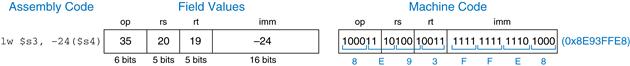
Figure 6.10 Machine code for an l-type instruction
I-type instructions have a 16-bit immediate field, but the immediates are used in 32-bit operations. For example, lw adds a 16-bit offset to a 32-bit base register. What should go in the upper half of the 32 bits? For positive immediates, the upper half should be all 0’s, but for negative immediates, the upper half should be all 1’s. Recall from Section 1.4.6 that this is called sign extension. An N-bit two’s complement number is sign-extended to an M-bit number (M > N) by copying the sign bit (most significant bit) of the N-bit number into all of the upper bits of the M-bit number. Sign-extending a two’s complement number does not change its value.
Most MIPS instructions sign-extend the immediate. For example, addi, lw, and sw do sign extension to support both positive and negative immediates. An exception to this rule is that logical operations (andi, ori, xori) place 0’s in the upper half; this is called zero extension rather than sign extension. Logical operations are discussed further in Section 6.4.1.
6.3.3 J-Type Instructions
The name J-type is short for jump-type. This format is used only with jump instructions (see Section 6.4.2). This instruction format uses a single 26-bit address operand, addr, as shown in Figure 6.11. Like other formats, J-type instructions begin with a 6-bit opcode. The remaining bits are used to specify an address, addr. Further discussion and machine code examples of J-type instructions are given in Sections 6.4.2 and 6.5.
![]()
Figure 6.11 J-type instruction format
6.3.4 Interpreting Machine Language Code
To interpret machine language, one must decipher the fields of each 32-bit instruction word. Different instructions use different formats, but all formats start with a 6-bit opcode field. Thus, the best place to begin is to look at the opcode. If it is 0, the instruction is R-type; otherwise it is I-type or J-type.
Example 6.5 Translating Machine Language to Assembly Language
Translate the following machine language code into assembly language.
0x2237FFF1
0x02F34022
Solution
First, we represent each instruction in binary and look at the six most significant bits to find the opcode for each instruction, as shown in Figure 6.12. The opcode determines how to interpret the rest of the bits. The opcodes are 0010002 (810) and 0000002 (010), indicating an addi and R-type instruction, respectively. The funct field of the R-type instruction is 1000102 (3410), indicating that it is a sub instruction. Figure 6.12 shows the assembly code equivalent of the two machine instructions.

Figure 6.12 Machine code to assembly code translation
6.3.5 The Power of the Stored Program
A program written in machine language is a series of 32-bit numbers representing the instructions. Like other binary numbers, these instructions can be stored in memory. This is called the stored program concept, and it is a key reason why computers are so powerful. Running a different program does not require large amounts of time and effort to reconfigure or rewire hardware; it only requires writing the new program to memory. Instead of dedicated hardware, the stored program offers general purpose computing. In this way, a computer can execute applications ranging from a calculator to a word processor to a video player simply by changing the stored program.
Instructions in a stored program are retrieved, or fetched, from memory and executed by the processor. Even large, complex programs are simplified to a series of memory reads and instruction executions.
Figure 6.13 shows how machine instructions are stored in memory. In MIPS programs, the instructions are normally stored starting at address 0x00400000. Remember that MIPS memory is byte-addressable, so 32-bit (4-byte) instruction addresses advance by 4 bytes, not 1.
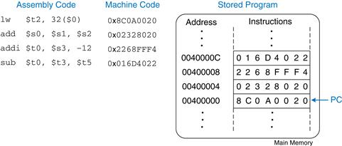
Figure 6.13 Stored program
To run or execute the stored program, the processor fetches the instructions from memory sequentially. The fetched instructions are then decoded and executed by the digital hardware. The address of the current instruction is kept in a 32-bit register called the program counter (PC). The PC is separate from the 32 registers shown previously in Table 6.1.
To execute the code in Figure 6.13, the operating system sets the PC to address 0x00400000. The processor reads the instruction at that memory address and executes the instruction, 0x8C0A0020. The processor then increments the PC by 4 to 0x00400004, fetches and executes that instruction, and repeats.
The architectural state of a microprocessor holds the state of a program. For MIPS, the architectural state consists of the register file and PC. If the operating system saves the architectural state at some point in the program, it can interrupt the program, do something else, then restore the state such that the program continues properly, unaware that it was ever interrupted. The architectural state is also of great importance when we build a microprocessor in Chapter 7.
Ada Lovelace, 1815–1852

Wrote the first computer program. It calculated the Bernoulli numbers using Charles Babbage’s Analytical Engine. She was the only legitimate child of the poet Lord Byron.
6.4 Programming
Software languages such as C or Java are called high-level programming languages because they are written at a more abstract level than assembly language. Many high-level languages use common software constructs such as arithmetic and logical operations, if/else statements, for and while loops, array indexing, and function calls. See Appendix C for more examples of these constructs in C. In this section, we explore how to translate these high-level constructs into MIPS assembly code.
6.4.1 Arithmetic/Logical Instructions
The MIPS architecture defines a variety of arithmetic and logical instructions. We introduce these instructions briefly here because they are necessary to implement higher-level constructs.
Logical Instructions
MIPS logical operations include and, or, xor, and nor. These R-type instructions operate bit-by-bit on two source registers and write the result to the destination register. Figure 6.14 shows examples of these operations on the two source values 0xFFFF0000 and 0x46A1F0B7. The figure shows the values stored in the destination register, rd, after the instruction executes.
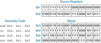
Figure 6.14 Logical operations
The and instruction is useful for masking bits (i.e., forcing unwanted bits to 0). For example, in Figure 6.14, 0xFFFF0000 AND 0x46A1F0B7 = 0x46A10000. The and instruction masks off the bottom two bytes and places the unmasked top two bytes of $s2, 0x46A1, in $s3. Any subset of register bits can be masked.
The or instruction is useful for combining bits from two registers. For example, 0x347A0000 OR 0x000072FC = 0x347A72FC, a combination of the two values.
MIPS does not provide a NOT instruction, but A NOR $0 = NOT A, so the NOR instruction can substitute.
Logical operations can also operate on immediates. These I-type instructions are andi, ori, and xori. nori is not provided, because the same functionality can be easily implemented using the other instructions, as will be explored in Exercise 6.16. Figure 6.15 shows examples of the andi, ori, and xori instructions. The figure gives the values of the source register and immediate and the value of the destination register rt after the instruction executes. Because these instructions operate on a 32-bit value from a register and a 16-bit immediate, they first zero-extend the immediate to 32 bits.
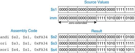
Figure 6.15 Logical operations with immediates
Shift Instructions
Shift instructions shift the value in a register left or right by up to 31 bits. Shift operations multiply or divide by powers of two. MIPS shift operations are sll (shift left logical), srl (shift right logical), and sra (shift right arithmetic).
As discussed in Section 5.2.5, left shifts always fill the least significant bits with 0’s. However, right shifts can be either logical (0’s shift into the most significant bits) or arithmetic (the sign bit shifts into the most significant bits). Figure 6.16 shows the machine code for the R-type instructions sll, srl, and sra. rt (i.e., $s1) holds the 32-bit value to be shifted, and shamt gives the amount by which to shift (4). The shifted result is placed in rd.

Figure 6.16 Shift instruction machine code
Figure 6.17 shows the register values for the shift instructions sll, srl, and sra. Shifting a value left by N is equivalent to multiplying it by 2N. Likewise, arithmetically shifting a value right by N is equivalent to dividing it by 2N, as discussed in Section 5.2.5.
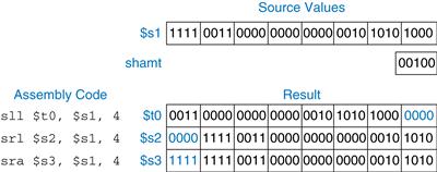
Figure 6.17 Shift operations
MIPS also has variable-shift instructions: sllv (shift left logical variable), srlv (shift right logical variable), and srav (shift right arithmetic variable). Figure 6.18 shows the machine code for these instructions. Variable-shift assembly instructions are of the form sllv rd, rt, rs. The order of rt and rs is reversed from most R-type instructions. rt ($s1) holds the value to be shifted, and the five least significant bits of rs ($s2) give the amount to shift. The shifted result is placed in rd, as before. The shamt field is ignored and should be all 0’s. Figure 6.19 shows register values for each type of variable-shift instruction.
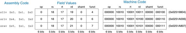
Figure 6.18 Variable-shift instruction machine code
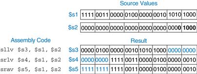
Figure 6.19 Variable-shift operations
Generating Constants
The addi instruction is helpful for assigning 16-bit constants, as shown in Code Example 6.10.
Code Example 6.10 16-BIT Constant
High-Level Code
int a = 0x4f3c;
MIPS Assembly Code
# $s0 = a
addi $s0, $0, 0x4f3c # a = 0x4f3c
To assign 32-bit constants, use a load upper immediate instruction (lui) followed by an or immediate (ori) instruction as shown in Code Example 6.11. lui loads a 16-bit immediate into the upper half of a register and sets the lower half to 0. As mentioned earlier, ori merges a 16-bit immediate into the lower half.
The int data type in C refers to a word of data representing a two’s complement integer.
MIPS uses 32-bit words, so an int represents a number in the range [−231, 231− 1].
Code Example 6.11 32-BIT Constant
High-Level Code
int a = 0x6d5e4f3c;
MIPS Assembly Code
# $s0 = a
lui $s0, 0x6d5e # a = 0x6d5e0000
ori $s0, $s0, 0x4f3c # a = 0x6d5e4f3c
Multiplication and Division Instructions*
Multiplication and division are somewhat different from other arithmetic operations. Multiplying two 32-bit numbers produces a 64-bit product. Dividing two 32-bit numbers produces a 32-bit quotient and a 32-bit remainder.
hi and lo are not among the usual 32 MIPS registers, so special instructions are needed to access them. mfhi $s2 (move from hi) copies the value in hi to $s2. mflo $s3 (move from lo) copies the value in lo to $s3. hi and lo are technically part of the architectural state; however, we generally ignore these registers in this book.
The MIPS architecture has two special-purpose registers, hi and lo, which are used to hold the results of multiplication and division. mult $s0, $s1 multiplies the values in $s0 and $s1. The 32 most significant bits of the product are placed in hi and the 32 least significant bits are placed in lo. Similarly, div $s0, $s1 computes $s0/$s1. The quotient is placed in lo and the remainder is placed in hi.
MIPS provides another multiply instruction that produces a 32-bit result in a general purpose register. mul $s1, $s2, $s3 multiplies the values in $s2 and $s3 and places the 32-bit result in $s1.
6.4.2 Branching
An advantage of a computer over a calculator is its ability to make decisions. A computer performs different tasks depending on the input. For example, if/else statements, switch/case statements, while loops, and for loops all conditionally execute code depending on some test.
To sequentially execute instructions, the program counter increments by 4 after each instruction. Branch instructions modify the program counter to skip over sections of code or to repeat previous code. Conditional branch instructions perform a test and branch only if the test is TRUE. Unconditional branch instructions, called jumps, always branch.
Conditional Branches
The MIPS instruction set has two conditional branch instructions: branch if equal (beq) and branch if not equal (bne). beq branches when the values in two registers are equal, and bne branches when they are not equal. Code Example 6.12 illustrates the use of beq. Note that branches are written as beq rs, rt, imm, where rs is the first source register. This order is reversed from most I-type instructions.
When the program in Code Example 6.12 reaches the branch if equal instruction (beq), the value in $s0 is equal to the value in $s1, so the branch is taken. That is, the next instruction executed is the add instruction just after the label called target. The two instructions directly after the branch and before the label are not executed.2
Assembly code uses labels to indicate instruction locations in the program. When the assembly code is translated into machine code, these labels are translated into instruction addresses (see Section 6.5). MIPS assembly labels are followed by a colon (:) and cannot use reserved words, such as instruction mnemonics. Most programmers indent their instructions but not the labels, to help make labels stand out.
Code Example 6.12 Conditional Branching using beq
MIPS Assembly Code
addi $s0, $0, 4 # $s0 = 0 + 4 = 4
addi $s1, $0, 1 # $s1 = 0 + 1 = 1
sll $s1, $s1, 2 # $s1 = 1 << 2 = 4
beq $s0, $s1, target # $s0 = = $s1, so branch is taken
addi $s1, $s1, 1 # not executed
sub $s1, $s1, $s0 # not executed
target:
add $s1, $s1, $s0 # $s1 = 4 + 4 = 8
Code Example 6.13 shows an example using the branch if not equal instruction (bne). In this case, the branch is not taken because $s0 is equal to $s1, and the code continues to execute directly after the bne instruction. All instructions in this code snippet are executed.
Code Example 6.13 Conditional Branching using bne
MIPS Assembly Code
addi $s0, $0, 4 # $s0 = 0 + 4 = 4
addi $s1, $0, 1 # $s1 = 0 + 1 = 1
s11 $s1, $s1, 2 # $s1 = 1 << 2 = 4
bne $s0, $s1, target # $s0 = = $s1, so branch is not taken
addi $s1, $s1, 1 # $s1 = 4 + 1 = 5
sub $s1, $s1, $s0 # $s1 = 5 − 4 = 1
target:
add $s1, $s1, $s0 # $s1 = 1 + 4 = 5
Jump
A program can unconditionally branch, or jump, using the three types of jump instructions: jump (j), jump and link (jal), and jump register (jr). Jump (j) jumps directly to the instruction at the specified label. Jump and link (jal) is similar to j but is used by functions to save a return address, as will be discussed in Section 6.4.6. Jump register (jr) jumps to the address held in a register. Code Example 6.14 shows the use of the jump instruction (j).
After the j target instruction, the program in Code Example 6.14 unconditionally continues executing the add instruction at the label target. All of the instructions between the jump and the label are skipped.
j and jal are J-type instructions. jr is an R-type instruction that uses only the rs operand.
Code Example 6.14 Unconditional Branching using j
MIPS Assembly Code
addi $s0, $0, 4 # $s0 = 4
addi $s1, $0, 1 # $s1 = 1
j target # jump to target
addi $s1, $s1, 1 # not executed
sub $s1, $s1, $s0 # not executed
target:
add $s1, $s1, $s0 # $s1 = 1 + 4 = 5
Code Example 6.15 Unconditional Branching using jr
MIPS Assembly Code
0x00002000 addi $s0, $0, 0x2010 # $s0 = 0x2010
0x00002004 jr $s0 # jump to 0x00002010
0x00002008 addi $s1, $0, 1 # not executed
0x0000200c sra $s1, $s1, 2 # not executed
0x00002010 lw $s3, 44($s1) # executed after jr instruction
Code Example 6.15 shows the use of the jump register instruction (jr). Instruction addresses are given to the left of each instruction. jr $s0 jumps to the address held in $s0, 0x00002010.
6.4.3 Conditional Statements
if, if/else, and switch/case statements are conditional statements commonly used in high-level languages. They each conditionally execute a block of code consisting of one or more statements. This section shows how to translate these high-level constructs into MIPS assembly language.
If Statements
An if statement executes a block of code, the if block, only when a condition is met. Code Example 6.16 shows how to translate an if statement into MIPS assembly code.
Code Example 6.16 if Statement
High-Level Code
if (i = = j)
f = g + h;
f = f – i;
MIPS Assembly Code
# $s0 = f, $s1 = g, $s2 = h, $s3 = i, $s4 = j
bne $s3, $s4, L1 # if i != j, skip if block
add $s0, $s1, $s2 # if block: f = g + h
L1:
sub $s0, $s0, $s3 # f = f − i
The assembly code for the if statement tests the opposite condition of the one in the high-level code. In Code Example 6.16, the high-level code tests for i == j, and the assembly code tests for i != j. The bne instruction branches (skips the if block) when i != j. Otherwise, i == j, the branch is not taken, and the if block is executed as desired.
If/Else Statements
if/else statements execute one of two blocks of code depending on a condition. When the condition in the if statement is met, the if block is executed. Otherwise, the else block is executed. Code Example 6.17 shows an example if/else statement.
Like if statements, if/else assembly code tests the opposite condition of the one in the high-level code. For example, in Code Example 6.17, the high-level code tests for i == j. The assembly code tests for the opposite condition (i != j). If that opposite condition is TRUE, bne skips the if block and executes the else block. Otherwise, the if block executes and finishes with a jump instruction (j) to jump past the else block.
Code Example 6.17 if/else Statement
High-Level Code
if (i = = j)
f = g + h;
else
f = f − i;
MIPS Assembly Code
# $s0 = f, $s1 = g, $s2 = h, $s3 = i, $s4 = j
bne $s3, $s4, else # if i != j, branch to else
add $s0, $s1, $s2 # if block: f = g + h
j L2 # skip past the else block
else:
sub $s0, $s0, $s3 # else block: f = f − i
L2:
Switch/Case Statements*
switch/case statements execute one of several blocks of code depending on the conditions. If no conditions are met, the default block is executed. A case statement is equivalent to a series of nested if/else statements. Code Example 6.18 shows two high-level code snippets with the same functionality: they calculate the fee for an ATM (automatic teller machine) withdrawal of $20, $50, or $100, as defined by amount. The MIPS assembly implementation is the same for both high-level code snippets.
6.4.4 Getting Loopy
Loops repeatedly execute a block of code depending on a condition. for loops and while loops are common loop constructs used by high-level languages. This section shows how to translate them into MIPS assembly language.
Code Example 6.18 switch/case Statement
High-Level Code
switch (amount) {
case 20: fee = 2; break;
case 50: fee = 3; break;
case 100: fee = 5; break;
default: fee = 0;
}
// equivalent function using if/else statements
if (amount = = 20) fee = 2;
else if (amount = = 50) fee = 3;
else if (amount = = 100) fee = 5;
else fee = 0;
MIPS Assembly Code
# $s0 = amount, $s1 = fee
case20:
addi $t0, $0, 20 # $t0 = 20
bne $s0, $t0, case50 # amount = = 20? if not,
# skip to case50
addi $s1, $0, 2 # if so, fee = 2
j done # and break out of case
case50:
addi $t0, $0, 50 # $t0 = 50
bne $s0, $t0, case100 # amount = = 50? if not,
# skip to case100
addi $s1, $0, 3 # if so, fee = 3
j done # and break out of case
case100:
addi $t0, $0, 100 # $t0 = 100
bne $s0, $t0, default # amount = = 100? if not,
# skip to default
addi $s1, $0, 5 # if so, fee = 5
j done # and break out of case
default:
add $s1, $0, $0 # fee = 0
done:
While Loops
while loops repeatedly execute a block of code until a condition is not met. The while loop in Code Example 6.19 determines the value of x such that 2x = 128. It executes seven times, until pow = 128.
Like if/else statements, the assembly code for while loops tests the opposite condition of the one given in the high-level code. If that opposite condition is TRUE, the while loop is finished.
Code Example 6.19 while Loop
High-Level Code
int pow = 1;
int x = 0;
while (pow != 128)
{
pow = pow * 2;
x = x + 1;
}
MIPS Assembly Code
# $s0 = pow, $s1 = x
addi $s0, $0, 1 # pow = 1
addi $s1, $0, 0 # x = 0
addi $t0, $0, 128 # t0 = 128 for comparison
while:
beq $s0, $t0, done # if pow = = 128, exit while loop
sll $s0, $s0, 1 # pow = pow * 2
addi $s1, $s1, 1 # x = x + 1
j while
done:
In Code Example 6.19, the while loop compares pow to 128 and exits the loop if it is equal. Otherwise it doubles pow (using a left shift), increments x, and jumps back to the start of the while loop.
do/while loops are similar to while loops except they execute the loop body once before checking the condition. They are of the form:
do
statement
while (condition);
For Loops
for loops, like while loops, repeatedly execute a block of code until a condition is not met. However, for loops add support for a loop variable, which typically keeps track of the number of loop executions. A general format of the for loop is
for (initialization; condition; loop operation)
statement
The initialization code executes before the for loop begins. The condition is tested at the beginning of each loop. If the condition is not met, the loop exits. The loop operation executes at the end of each loop.
Code Example 6.20 adds the numbers from 0 to 9. The loop variable, in this case i, is initialized to 0 and is incremented at the end of each loop iteration. At the beginning of each iteration, the for loop executes only when i is not equal to 10. Otherwise, the loop is finished. In this case, the for loop executes 10 times. for loops can be implemented using a while loop, but the for loop is often convenient.
Magnitude Comparison
So far, the examples have used beq and bne to perform equality or inequality comparisons and branches. MIPS provides the set less than instruction, slt, for magnitude comparison. slt sets rd to 1 when rs < rt. Otherwise, rd is 0.
Code Example 6.20 for Loop
High-Level Code
int sum = 0;
for (i = 0; i != 10; i = i + 1) {
sum = sum + i ;
}
// equivalent to the following while loop
int sum = 0;
int i = 0;
while (i != 10) {
sum = sum + i;
i = i + 1;
}
MIPS Assembly Code
# $s0 = i, $s1 = sum
add $s1, $0, $0 # sum = 0
addi $s0, $0, 0 # i = 0
addi $t0, $0, 10 # $t0 = 10
for:
beq $s0, $t0, done # if i = = 10, branch to done
add $s1, $s1, $s0 # sum = sum + i
addi $s0, $s0, 1 # increment i
j for
done:
Example 6.6 Loops Using slt
The following high-level code adds the powers of 2 from 1 to 100. Translate it into assembly language.
// high-level code
int sum = 0;
for (i = 1; i < 101; i = i * 2)
sum = sum + i;
Solution
The assembly language code uses the set less than (slt) instruction to perform the less than comparison in the for loop.
# MIPS assembly code
# $s0 = i, $s1 = sum
addi $s1, $0, 0 # sum = 0
addi $s0, $0, 1 # i = 1
addi $t0, $0, 101 # $t0 = 101
loop:
slt $t1, $s0, $t0 # if (i < 101) $t1 = 1, else $t1 = 0
beq $t1, $0, done # if $t1 == 0 (i >= 101), branch to done
add $s1, $s1, $s0 # sum = sum + i
sll $s0, $s0, 1 # i = i * 2
j loop
done:
Exercise 6.17 explores how to use slt for other magnitude comparisons including greater than, greater than or equal, and less than or equal.
6.4.5 Arrays
Arrays are useful for accessing large amounts of similar data. An array is organized as sequential data addresses in memory. Each array element is identified by a number called its index. The number of elements in the array is called the size of the array. This section shows how to access array elements in memory.
Array Indexing
Figure 6.20 shows an array of five integers stored in memory. The index ranges from 0 to 4. In this case, the array is stored in a processor’s main memory starting at base address 0x10007000. The base address gives the address of the first array element, array[0].
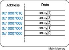
Figure 6.20 Five-entry array with base address of 0x10007000
Code Example 6.21 multiplies the first two elements in array by 8 and stores them back into the array.
The first step in accessing an array element is to load the base address of the array into a register. Code Example 6.21 loads the base address into $s0. Recall that the load upper immediate (lui) and or immediate (ori) instructions can be used to load a 32-bit constant into a register.
Code Example 6.21 Accessing Arrays
High-Level Code
int array[5];
array[0] = array[0] * 8;
array[1] = array[1] * 8;
MIPS Assembly Code
# $s0 = base address of array
lui $s0, 0x1000 # $s0 = 0x10000000
ori $s0, $s0, 0x7000 # $s0 = 0x10007000
lw $t1, 0($s0) # $t1 = array[0]
sll $t1, $t1, 3 # $t1 = $t1 << 3 = $t1 * 8
sw $t1, 0($s0) # array[0] = $t1
Iw $t1, 4($s0) # $t1 = array[1]
sll $t1, $t1, 3 # $t1 = $t1 << 3 = $t1 * 8
sw $t1, 4($s0) # array[1] = $t1
Code Example 6.21 also illustrates why lw takes a base address and an offset. The base address points to the start of the array. The offset can be used to access subsequent elements of the array. For example, array[1] is stored at memory address 0x10007004 (one word or four bytes after array[0]), so it is accessed at an offset of 4 past the base address.
You might have noticed that the code for manipulating each of the two array elements in Code Example 6.21 is essentially the same except for the index. Duplicating the code is not a problem when accessing two array elements, but it would become terribly inefficient for accessing all of the elements in a large array. Code Example 6.22 uses a for loop to multiply by 8 all of the elements of a 1000-element array stored at a base address of 0x23B8F000.
Figure 6.21 shows the 1000-element array in memory. The index into the array is now a variable (i) rather than a constant, so we cannot take advantage of the immediate offset in lw. Instead, we compute the address of the ith element and store it in $t0. Remember that each array element is a word but that memory is byte addressed, so the offset from the base address is i * 4. Shifting left by 2 is a convenient way to multiply by 4 in MIPS assembly language. This example readily extends to an array of any size.
Code Example 6.22 Accessing Arrays using a for Loop
High-Level Code
int i;
int array[1000];
for (i = 0; i < 1000; i = i + 1)
array[i] = array[i] * 8;
MIPS Assembly Code
# $s0 = array base address, $s1 = i
# initialization code
lui $s0, 0x23B8 # $s0 = 0x23B80000
ori $s0, $s0, 0xF000 # $s0 = 0x23B8F000
addi $s1, $0, 0 # i = 0
addi $t2, $0, 1000 # $t2 = 1000
loop:
slt $t0, $s1, $t2 # i < 1000?
beq $t0, $0, done # if not, then done
sll $t0, $s1, 2 # $t0 = i*4 (byte offset)
add $t0, $t0, $s0 # address of array[i]
lw $t1, 0($t0) # $t1 = array[i]
sll $t1, $t1, 3 # $t1 = array[i] * 8
sw $t1, 0($t0) # array[i] = array[i] * 8
addi $s1, $s1, 1 # i = i + 1
j loop # repeat
done:

Figure 6.21 Memory holding array[1000] starting at base address 0x23B8F000
Bytes and Characters
Numbers in the range [ –128, 127] can be stored in a single byte rather than an entire word. Because there are much fewer than 256 characters on an English language keyboard, English characters are often represented by bytes. The C language uses the type char to represent a byte or character.
Other programming languages, such as Java, use different character encodings, most notably Unicode. Unicode uses 16 bits to represent each character, so it supports accents, umlauts, and Asian languages. For more information, see www.unicode.org.
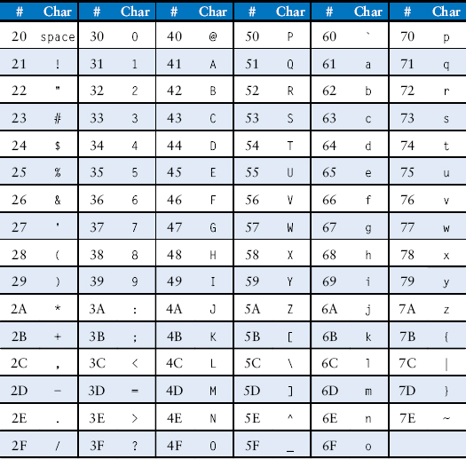
Early computers lacked a standard mapping between bytes and English characters, so exchanging text between computers was difficult. In 1963, the American Standards Association published the American Standard Code for Information Interchange (ASCII), which assigns each text character a unique byte value. Table 6.2 shows these character encodings for printable characters. The ASCII values are given in hexadecimal. Lower-case and upper-case letters differ by 0x20 (32).
Table 6.2 ASCII encodings
MIPS provides load byte and store byte instructions to manipulate bytes or characters of data: load byte unsigned (lbu), load byte (lb), and store byte (sb). All three are illustrated in Figure 6.22.
ASCII codes developed from earlier forms of character encoding. Beginning in 1838, telegraph machines used Morse code, a series of dots (.) and dashes (–), to represent characters. For example, the letters A, B, C, and D were represented as . – , – … , – . – . , and – . . , respectively. The number of dots and dashes varied with each letter. For efficiency, common letters used shorter codes.
In 1874, Jean-Maurice-Emile Baudot invented a 5-bit code called the Baudot code. For example, A, B, C, and D were represented as 00011, 11001, 01110, and 01001. However, the 32 possible encodings of this 5-bit code were not sufficient for all the English characters. But 8-bit encoding was. Thus, as electronic communication became prevalent, 8-bit ASCII encoding emerged as the standard.
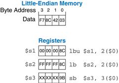
Figure 6.22 Instructions for loading and storing bytes
Load byte unsigned (lbu) zero-extends the byte, and load byte (lb) sign-extends the byte to fill the entire 32-bit register. Store byte (sb) stores the least significant byte of the 32-bit register into the specified byte address in memory. In Figure 6.22, lbu loads the byte at memory address 2 into the least significant byte of $s1 and fills the remaining register bits with 0. lb loads the sign-extended byte at memory address 2 into $s2. sb stores the least significant byte of $s3 into memory byte 3; it replaces 0xF7 with 0x9B. The more significant bytes of $s3 are ignored.
Example 6.7 Using lb and sb to Access a Character Array
The following high-level code converts a ten-entry array of characters from lower-case to upper-case by subtracting 32 from each array entry. Translate it into MIPS assembly language. Remember that the address difference between array elements is now 1 byte, not 4 bytes. Assume that $s0 already holds the base address of chararray.
// high-level code
char chararray[10];
int i;
for (i = 0; i != 10; i = i + 1)
chararray[i] = chararray[i] – 32;
Solution
# MIPS assembly code
# $s0 = base address of chararray, $s1 = i
addi $s1, $0, 0 # i = 0
addi $t0, $0, 10 # $t0 = 10
loop: beq $t0, $s1, done # if i = = 10, exit loop
add $t1, $s1, $s0 # $t1 = address of chararray[i]
lb $t2, 0($t1) # $t2 = array[i]
addi $t2, $t2, –32 # convert to upper case: $t2 = $t2 − 32
sb $t2, 0($t1) # store new value in array:
# chararray[i] = $t2
addi $s1, $s1, 1 # i = i+1
j loop # repeat
done:
A series of characters is called a string. Strings have a variable length, so programming languages must provide a way to determine the length or end of the string. In C, the null character (0x00) signifies the end of a string. For example, Figure 6.23 shows the string “Hello!” (0x48 65 6C 6C 6F 21 00) stored in memory. The string is seven bytes long and extends from address 0x1522FFF0 to 0x1522FFF6. The first character of the string (H = 0x48) is stored at the lowest byte address (0x1522FFF0).

Figure 6.23 The string “Hello!” stored in memory
6.4.6 Function Calls
High-level languages often use functions (also called procedures) to reuse frequently accessed code and to make a program more modular and readable. Functions have inputs, called arguments, and an output, called the return value. Functions should calculate the return value and cause no other unintended side effects.
When one function calls another, the calling function, the caller, and the called function, the callee, must agree on where to put the arguments and the return value. In MIPS, the caller conventionally places up to four arguments in registers $a0–$a3 before making the function call, and the callee places the return value in registers $v0–$v1 before finishing. By following this convention, both functions know where to find the arguments and return value, even if the caller and callee were written by different people.
The callee must not interfere with the function of the caller. Briefly, this means that the callee must know where to return to after it completes and it must not trample on any registers or memory needed by the caller. The caller stores the return address in $ra at the same time it jumps to the callee using the jump and link instruction (jal). The callee must not overwrite any architectural state or memory that the caller is depending on. Specifically, the callee must leave the saved registers, $s0–$s7, $ra, and the stack, a portion of memory used for temporary variables, unmodified.
This section shows how to call and return from a function. It shows how functions access input arguments and the return value and how they use the stack to store temporary variables.
Function Calls and Returns
MIPS uses the jump and link instruction (jal) to call a function and the jump register instruction (jr) to return from a function. Code Example 6.23 shows the main function calling the simple function. main is the caller, and simple is the callee. The simple function is called with no input arguments and generates no return value; it simply returns to the caller. In Code Example 6.23, instruction addresses are given to the left of each MIPS instruction in hexadecimal.
Code Example 6.23 simple Function Call
High-Level Code
int main() {
simple();
…
}
// void means the function returns no value
void simple() {
return;
}
MIPS Assembly Code
0x00400200 main: jal simple # call function
0x00400204 …
0x00401020 simple: jr $ra # return
Jump and link (jal) and jump register (jr $ra) are the two essential instructions needed for a function call. jal performs two operations: it stores the address of the next instruction (the instruction after jal) in the return address register ($ra), and it jumps to the target instruction.
In Code Example 6.23, the main function calls the simple function by executing the jump and link (jal) instruction. jal jumps to the simple label and stores 0x00400204 in $ra. The simple function returns immediately by executing the instruction jr $ra, jumping to the instruction address held in $ra. The main function then continues executing at this address (0x00400204).
Input Arguments and Return Values
The simple function in Code Example 6.23 is not very useful, because it receives no input from the calling function (main) and returns no output. By MIPS convention, functions use $a0–$a3 for input arguments and $v0–$v1 for the return value. In Code Example 6.24, the function diffofsums is called with four arguments and returns one result.
According to MIPS convention, the calling function, main, places the function arguments from left to right into the input registers, $a0–$a3. The called function, diffofsums, stores the return value in the return register, $v0.
A function that returns a 64-bit value, such as a double-precision floating point number, uses both return registers, $v0 and $v1. When a function with more than four arguments is called, the additional input arguments are placed on the stack, which we discuss next.
Code Example 6.24 has some subtle errors. Code Examples 6.25 and 6.26 on pages 328 and 329 show improved versions of the program.
Code Example 6.24 Function Call with Arguments and Return Values
High-Level Code
int main()
{
int y;
…
y = diffofsums(2, 3, 4, 5);
…
}
int diffofsums(int f, int g, int h, int i)
{
int result;
result = (f + g) − (h + i);
return result;
}
MIPS Assembly Code
# $s0 = y
main:
…
addi $a0, $0, 2 # argument 0 = 2
addi $a1, $0, 3 # argument 1 = 3
addi $a2, $0, 4 # argument 2 = 4
addi $a3, $0, 5 # argument 3 = 5
jal diffofsums # call function
add $s0, $v0, $0 # y = returned value
…
# $s0 = result
diffofsums:
add $t0, $a0, $a1 # $t0 = f + g
add $t1, $a2, $a3 # $t1 = h + i
sub $s0, $t0, $t1 # result = (f + g) − (h + i)
add $v0, $s0, $0 # put return value in $v0
jr $ra # return to caller
The Stack
The stack is memory that is used to save local variables within a function. The stack expands (uses more memory) as the processor needs more scratch space and contracts (uses less memory) when the processor no longer needs the variables stored there. Before explaining how functions use the stack to store temporary variables, we explain how the stack works.
The stack is a last-in-first-out (LIFO) queue. Like a stack of dishes, the last item pushed onto the stack (the top dish) is the first one that can be pulled (popped) off. Each function may allocate stack space to store local variables but must deallocate it before returning. The top of the stack, is the most recently allocated space. Whereas a stack of dishes grows up in space, the MIPS stack grows down in memory. The stack expands to lower memory addresses when a program needs more scratch space.

Figure 6.24 shows a picture of the stack. The stack pointer, $sp, is a special MIPS register that points to the top of the stack. A pointer is a fancy name for a memory address. It points to (gives the address of) data. For example, in Figure 6.24(a) the stack pointer, $sp, holds the address value 0x7FFFFFFC and points to the data value 0x12345678. $sp points to the top of the stack, the lowest accessible memory on the stack. Thus, in Figure 6.24(a), the stack cannot access memory below memory word 0x7FFFFFFC.
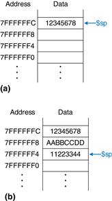
Figure 6.24 The stack
The stack pointer ($sp) starts at a high memory address and decrements to expand as needed. Figure 6.24(b) shows the stack expanding to allow two more data words of temporary storage. To do so, $sp decrements by 8 to become 0x7FFFFFF4. Two additional data words, 0xAABBCCDD and 0x11223344, are temporarily stored on the stack.
One of the important uses of the stack is to save and restore registers that are used by a function. Recall that a function should calculate a return value but have no other unintended side effects. In particular, it should not modify any registers besides the one containing the return value $v0. The diffofsums function in Code Example 6.24 violates this rule because it modifies $t0, $t1, and $s0. If main had been using $t0, $t1, or $s0 before the call to diffofsums, the contents of these registers would have been corrupted by the function call.
To solve this problem, a function saves registers on the stack before it modifies them, then restores them from the stack before it returns. Specifically, it performs the following steps.
1. Makes space on the stack to store the values of one or more registers.
2. Stores the values of the registers on the stack.
3. Executes the function using the registers.
4. Restores the original values of the registers from the stack.
Code Example 6.25 shows an improved version of diffofsums that saves and restores $t0, $t1, and $s0. The new lines are indicated in blue. Figure 6.25 shows the stack before, during, and after a call to the diffofsums function from Code Example 6.25. diffofsums makes room for three words on the stack by decrementing the stack pointer $sp by 12. It then stores the current values of $s0, $t0, and $t1 in the newly allocated space. It executes the rest of the function, changing the values in these three registers. At the end of the function, diffofsums restores the values of $s0, $t0, and $t1 from the stack, deallocates its stack space, and returns. When the function returns, $v0 holds the result, but there are no other side effects: $s0, $t0, $t1, and $sp have the same values as they did before the function call.

Figure 6.25 The stack (a) before, (b) during, and (c) after diffofsums function call
The stack space that a function allocates for itself is called its stack frame. diffofsums’s stack frame is three words deep. The principle of modularity tells us that each function should access only its own stack frame, not the frames belonging to other functions.
Code Example 6.25 Function Saving Registers on the Stack
MIPS Assembly Code
# $s0 = result
diffofsums:
addi $sp, $sp, −12 # make space on stack to store three registers
sw $s0, 8($sp) # save $s0 on stack
sw $t0, 4($sp) # save $t0 on stack
sw $t1, 0($sp) # save $t1 on stack
add $t0, $a0, $a1 # $t0 = f + g
add $t1, $a2, $a3 # $t1 = h + i
sub $s0, $t0, $t1 # result = (f + g) − (h + i)
add $v0, $s0, $0 # put return value in $v0
lw $t1, 0($sp) # restore $t1 from stack
lw $t0, 4($sp) # restore $t0 from stack
lw $s0, 8($sp) # restore $s0 from stack
addi $sp, $sp, 12 # deallocate stack space
jr $ra # return to caller
Preserved Registers
Code Example 6.25 assumes that temporary registers $t0 and $t1 must be saved and restored. If the calling function does not use those registers, the effort to save and restore them is wasted. To avoid this waste, MIPS divides registers into preserved and nonpreserved categories. The preserved registers include $s0–$s7 (hence their name, saved). The nonpreserved registers include $t0–$t9 (hence their name, temporary). A function must save and restore any of the preserved registers that it wishes to use, but it can change the nonpreserved registers freely.
Code Example 6.26 shows a further improved version of diffofsums that saves only $s0 on the stack. $t0 and $t1 are nonpreserved registers, so they need not be saved.
Remember that when one function calls another, the former is the caller and the latter is the callee. The callee must save and restore any preserved registers that it wishes to use. The callee may change any of the nonpreserved registers. Hence, if the caller is holding active data in a nonpreserved register, the caller needs to save that nonpreserved register before making the function call and then needs to restore it afterward. For these reasons, preserved registers are also called callee-save, and nonpreserved registers are called caller-save.
Code Example 6.26 Function Saving Preserved Registers on the Stack
MIPS Assembly Code
# $s0 = result
diffofsums
addi $sp, $sp, −4 # make space on stack to store one register
sw $s0, 0($sp) # save $s0 on stack
add $t0, $a0, $a1 # $t0 = f + g
add $t1, $a2, $a3 # $t1 = h + i
sub $s0, $t0, $t1 # result = (f + g) − (h + i)
add $v0, $s0, $0 # put return value in $v0
lw $s0, 0($sp) # restore $s0 from stack
addi $sp, $sp, 4 # deallocate stack space
jr $ra # return to caller
Table 6.3 summarizes which registers are preserved. $s0–$s7 are generally used to hold local variables within a function, so they must be saved. $ra must also be saved, so that the function knows where to return. $t0–$t9 are used to hold temporary results before they are assigned to local variables. These calculations typically complete before a function call is made, so they are not preserved, and it is rare that the caller needs to save them. $a0–$a3 are often overwritten in the process of calling a function. Hence, they must be saved by the caller if the caller depends on any of its own arguments after a called function returns. $v0–$v1 certainly should not be preserved, because the callee returns its result in these registers.
Table 6.3 Preserved and nonpreserved registers
| Preserved | Nonpreserved |
| Saved registers: $s0–$s7 | Temporary registers: $t0–$t9 |
| Return address: $ra | Argument registers: $a0–$a3 |
| Stack pointer: $sp | Return value registers: $v0–$v1 |
| Stack above the stack pointer | Stack below the stack pointer |
The stack above the stack pointer is automatically preserved as long as the callee does not write to memory addresses above $sp. In this way, it does not modify the stack frame of any other functions. The stack pointer itself is preserved, because the callee deallocates its stack frame before returning by adding back the same amount that it subtracted from $sp at the beginning of the function.
Recursive Function Calls
A function that does not call others is called a leaf function; an example is diffofsums. A function that does call others is called a nonleaf function. As mentioned earlier, nonleaf functions are somewhat more complicated because they may need to save nonpreserved registers on the stack before they call another function, and then restore those registers afterward. Specifically, the caller saves any non-preserved registers ($t0–$t9 and $a0–$a3) that are needed after the call. The callee saves any of the preserved registers ($s0–$s7 and $ra) that it intends to modify.
A recursive function is a nonleaf function that calls itself. The factorial function can be written as a recursive function call. Recall that factorial(n) = n × (n – 1) × (n – 2) × … × 2 × 1. The factorial function can be rewritten recursively as factorial(n) = n × factorial(n – 1). The factorial of 1 is simply 1. Code Example 6.27 shows the factorial function written as a recursive function. To conveniently refer to program addresses, we assume that the program starts at address 0x90.
The factorial function might modify $a0 and $ra, so it saves them on the stack. It then checks whether n < 2. If so, it puts the return value of 1 in $v0, restores the stack pointer, and returns to the caller. It does not have to reload $ra and $a0 in this case, because they were never modified. If n > 1, the function recursively calls factorial(n ‒ 1). It then restores the value of n ($a0) and the return address ($ra) from the stack, performs the multiplication, and returns this result. The multiply instruction (mul $v0, $a0, $v0) multiplies $a0 and $v0 and places the result in $v0.
Code Example 6.27 factorial Recursive Function Call
High-Level Code
int factorial(int n) {
if (n <= 1)
return 1;
else
return (n * factorial(n − 1));
}
MIPS Assembly Code
0x90 factorial: addi $sp, $sp, −8 # make room on stack
0x94 sw $a0, 4($sp) # store $a0
0x98 sw $ra, 0($sp) # store $ra
0x9C addi $t0, $0, 2 # $t0 = 2
OxAO slt $t0, $a0, $t0 # n <= 1 ?
0xA4 beq $t0, $0, else # no: goto else
0xA8 addi $v0, $0, 1 # yes: return 1
OxAC addi $sp, $sp, 8 # restore $sp
OxBO jr $ra # return
0xB4 else: addi $a0, $a0, −1 # n = n − 1
0xB8 jal factorial # recursive call
OxBC Iw $ra, 0($sp) # restore $ra
OxCO Iw $a0, 4($sp) # restore $a0
0xC4 addi $sp, $sp, 8 # restore $sp
0xC8 mul $v0, $a0, $v0 # n * factorial(n−1)
OxCC jr $ra # return
Figure 6.26 shows the stack when executing factorial(3). We assume that $sp initially points to 0xFC, as shown in Figure 6.26(a). The function creates a two-word stack frame to hold $a0 and $ra. On the first invocation, factorial saves $a0 (holding n = 3) at 0xF8 and $ra at 0xF4, as shown in Figure 6.26(b). The function then changes $a0 to n = 2 and recursively calls factorial(2), making $ra hold 0xBC. On the second invocation, it saves $a0 (holding n = 2) at 0xF0 and $ra at 0xEC. This time, we know that $ra contains 0xBC. The function then changes $a0 to n = 1 and recursively calls factorial(1). On the third invocation, it saves $a0 (holding n = 1) at 0xE8 and $ra at 0xE4. This time, $ra again contains 0xBC. The third invocation of factorial returns the value 1 in $v0 and deallocates the stack frame before returning to the second invocation. The second invocation restores n to 2, restores $ra to 0xBC (it happened to already have this value), deallocates the stack frame, and returns $v0 = 2 × 1 = 2 to the first invocation. The first invocation restores n to 3, restores $ra to the return address of the caller, deallocates the stack frame, and returns $v0 = 3 × 2 = 6. Figure 6.26(c) shows the stack as the recursively called functions return. When factorial returns to the caller, the stack pointer is in its original position (0xFC), none of the contents of the stack above the pointer have changed, and all of the preserved registers hold their original values. $v0 holds the return value, 6.
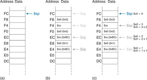
Figure 6.26 Stack during factorial function call when n = 3: (a) before call, (b) after last recursive call, (c) after return
Additional Arguments and Local Variables*
Functions may have more than four input arguments and local variables. The stack is used to store these temporary values. By MIPS convention, if a function has more than four arguments, the first four are passed in the argument registers as usual. Additional arguments are passed on the stack, just above $sp. The caller must expand its stack to make room for the additional arguments. Figure 6.27(a) shows the caller’s stack for calling a function with more than four arguments.

Figure 6.27 Stack usage: (a) before call, (b) after call
A function can also declare local variables or arrays. Local variables are declared within a function and can be accessed only within that function. Local variables are stored in $s0–$s7; if there are too many local variables, they can also be stored in the function’s stack frame. In particular, local arrays are stored on the stack.
Figure 6.27(b) shows the organization of a callee’s stack frame. The stack frame holds the function’s own arguments, the return address, and any of the saved registers that the function will modify. It also holds local arrays and any excess local variables. If the callee has more than four arguments, it finds them in the caller’s stack frame. Accessing additional input arguments is the one exception in which a function can access stack data not in its own stack frame.
6.5 Addressing Modes
MIPS uses five addressing modes: register-only, immediate, base, PC-relative, and pseudo-direct. The first three modes (register-only, immediate, and base addressing) define modes of reading and writing operands. The last two (PC-relative and pseudo-direct addressing) define modes of writing the program counter, PC.
Register-Only Addressing
Register-only addressing uses registers for all source and destination operands. All R-type instructions use register-only addressing.
Immediate Addressing
Immediate addressing uses the 16-bit immediate along with registers as operands. Some I-type instructions, such as add immediate (addi) and load upper immediate (lui), use immediate addressing.
Base Addressing
Memory access instructions, such as load word (lw) and store word (sw), use base addressing. The effective address of the memory operand is found by adding the base address in register rs to the sign-extended 16-bit offset found in the immediate field.
PC-Relative Addressing
Conditional branch instructions use PC-relative addressing to specify the new value of the PC if the branch is taken. The signed offset in the immediate field is added to the PC to obtain the new PC; hence, the branch destination address is said to be relative to the current PC.
Code Example 6.28 shows part of the factorial function from Code Example 6.27. Figure 6.28 shows the machine code for the beq instruction. The branch target address (BTA) is the address of the next instruction to execute if the branch is taken. The beq instruction in Figure 6.28 has a BTA of 0xB4, the instruction address of the else label.

Figure 6.28 Machine code for beq
The 16-bit immediate field gives the number of instructions between the BTA and the instruction after the branch instruction (the instruction at PC + 4). In this case, the value in the immediate field of beq is 3 because the BTA (0xB4) is 3 instructions past PC + 4 (0xA8).
The processor calculates the BTA from the instruction by sign-extending the 16-bit immediate, multiplying it by 4 (to convert words to bytes), and adding it to PC + 4.
Code Example 6.28 Calculating the Branch Target Address
MIPS Assembly Code
0xA4 beq $t0, $0, else
0xA8 addi $v0, $0, 1
0xAC addi $sp, $sp, 8
0xBO jr $ra
0xB4 else: addi $a0, $a0, −1
0xB8 jal factorial
Example 6.8 Calculating the Immediate Field for Pc-Relative Addressing
Calculate the immediate field and show the machine code for the branch not equal (bne) instruction in the following program.
# MIPS assembly code
0x40 loop: add $t1, $a0, $s0
0x44 lb $t1, 0($t1)
0x48 add $t2, $a1, $s0
0x4C sb $t1, 0($t2)
0x50 addi $s0, $s0, 1
0x54 bne $t1, $0, loop
0x58 lw $s0, 0($sp)
Solution
Figure 6.29 shows the machine code for the bne instruction. Its branch target address, 0x40, is 6 instructions behind PC + 4 (0x58), so the immediate field is –6.

Figure 6.29 bne machine code
Pseudo-Direct Addressing
In direct addressing, an address is specified in the instruction. The jump instructions, j and jal, ideally would use direct addressing to specify a 32-bit jump target address (JTA) to indicate the instruction address to execute next.
Code Example 6.29 Calculating the Jump Target Address
MIPS Assembly Code
0x0040005C jal sum
…
0x004000A0 sum: add $v0, $a0, $a1
Unfortunately, the J-type instruction encoding does not have enough bits to specify a full 32-bit JTA. Six bits of the instruction are used for the opcode, so only 26 bits are left to encode the JTA. Fortunately, the two least significant bits, JTA1:0, should always be 0, because instructions are word aligned. The next 26 bits, JTA27:2, are taken from the addr field of the instruction. The four most significant bits, JTA31:28, are obtained from the four most significant bits of PC + 4. This addressing mode is called pseudo-direct.
Code Example 6.29 illustrates a jal instruction using pseudo-direct addressing. The JTA of the jal instruction is 0x004000A0. Figure 6.30 shows the machine code for this jal instruction. The top four bits and bottom two bits of the JTA are discarded. The remaining bits are stored in the 26-bit address field (addr).
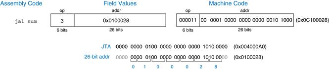
Figure 6.30 jal machine code
The processor calculates the JTA from the J-type instruction by appending two 0’s and prepending the four most significant bits of PC + 4 to the 26-bit address field (addr).
Because the four most significant bits of the JTA are taken from PC + 4, the jump range is limited. The range limits of branch and jump instructions are explored in Exercises 6.29 to 6.32. All J-type instructions, j and jal, use pseudo-direct addressing.
Note that the jump register instruction, jr, is not a J-type instruction. It is an R-type instruction that jumps to the 32-bit value held in register rs.
6.6 Lights, Camera, Action: Compiling, Assembling, and Loading
Up until now, we have shown how to translate short high-level code snippets into assembly and machine code. This section describes how to compile and assemble a complete high-level program and how to load the program into memory for execution.
We begin by introducing the MIPS memory map, which defines where code, data, and stack memory are located. We then show the steps of code execution for a sample program.
6.6.1 The Memory Map
With 32-bit addresses, the MIPS address space spans 232 bytes = 4 gigabytes (GB). Word addresses are divisible by 4 and range from 0 to 0xFFFFFFFC. Figure 6.31 shows the MIPS memory map. The MIPS architecture divides the address space into four parts or segments: the text segment, global data segment, dynamic data segment, and reserved segments. The following sections describe each segment.
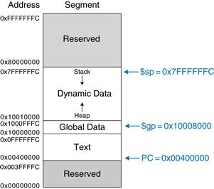
Figure 6.31 MIPS memory map
The Text Segment
The text segment stores the machine language program. It is large enough to accommodate almost 256 MB of code. Note that the four most significant bits of the address in the text space are all 0, so the j instruction can directly jump to any address in the program.
The Global Data Segment
The global data segment stores global variables that, in contrast to local variables, can be seen by all functions in a program. Global variables are defined at start-up, before the program begins executing. These variables are declared outside the main function in a C program and can be accessed by any function. The global data segment is large enough to store 64 KB of global variables.
Global variables are accessed using the global pointer ($gp), which is initialized to 0x100080000. Unlike the stack pointer ($sp), $gp does not change during program execution. Any global variable can be accessed with a 16-bit positive or negative offset from $gp. The offset is known at assembly time, so the variables can be efficiently accessed using base addressing mode with constant offsets.
The Dynamic Data Segment
The dynamic data segment holds the stack and the heap. The data in this segment are not known at start-up but are dynamically allocated and deallocated throughout the execution of the program. This is the largest segment of memory used by a program, spanning almost 2 GB of the address space.
As discussed in Section 6.4.6, the stack is used to save and restore registers used by functions and to hold local variables such as arrays. The stack grows downward from the top of the dynamic data segment (0x7FFFFFFC) and each stack frame is accessed in last-in-first-out order.
The heap stores data that is allocated by the program during runtime. In C, memory allocations are made by the malloc function; in C++ and Java, new is used to allocate memory. Like a heap of clothes on a dorm room floor, heap data can be used and discarded in any order. The heap grows upward from the bottom of the dynamic data segment.
If the stack and heap ever grow into each other, the program’s data can become corrupted. The memory allocator tries to ensure that this never happens by returning an out-of-memory error if there is insufficient space to allocate more dynamic data.
Grace Hopper, 1906–1992

Graduated from Yale University with a Ph.D. in mathematics. Developed the first compiler while working for the Remington Rand Corporation and was instrumental in developing the COBOL programming language. As a naval officer, she received many awards, including a World War II Victory Medal and the National Defense Service Medal.
The Reserved Segments
The reserved segments are used by the operating system and cannot directly be used by the program. Part of the reserved memory is used for interrupts (see Section 7.7) and for memory-mapped I/O (see Section 8.5).
6.6.2 Translating and Starting a Program
Figure 6.32 shows the steps required to translate a program from a high-level language into machine language and to start executing that program. First, the high-level code is compiled into assembly code. The assembly code is assembled into machine code in an object file. The linker combines the machine code with object code from libraries and other files to produce an entire executable program. In practice, most compilers perform all three steps of compiling, assembling, and linking. Finally, the loader loads the program into memory and starts execution. The remainder of this section walks through these steps for a simple program.

Figure 6.32 Steps for translating and starting a program
Step 1: Compilation
A compiler translates high-level code into assembly language. Code Example 6.30 shows a simple high-level program with three global variables and two functions, along with the assembly code produced by a typical compiler. The .data and .text keywords are assembler directives that indicate where the text and data segments begin. Labels are used for global variables f, g, and y. Their storage location will be determined by the assembler; for now, they are left as symbols in the code.
Code Example 6.30 Compiling a High-Level Program
High-Level Code
int f, g, y; // global variables
int main(void)
{
f = 2;
g = 3;
y = sum(f, g);
return y;
}
int sum(int a, int b) {
return (a + b);
}
MIPS Assembly Code
.data
f:
g:
y:
.text
main:
addi $sp, $sp, −4 # make stack frame
sw $ra, 0($sp) # store $ra on stack
addi $a0, $0, 2 # $a0 = 2
sw $a0, f # f = 2
addi $a1, $0, 3 # $a1 = 3
sw $a1, g # g = 3
jal sum # call sum function
sw $v0, y # y = sum(f, g)
Iw $ra, 0($sp) # restore $ra from stack
addi $sp, $sp, 4 # restore stack pointer
jr $ra # return to operating system
sum:
add $v0, $a0, $a1 # $v0 = a + b
jr $ra # return to caller
Step 2: Assembling
The assembler turns the assembly language code into an object file containing machine language code. The assembler makes two passes through the assembly code. On the first pass, the assembler assigns instruction addresses and finds all the symbols, such as labels and global variable names. The code after the first assembler pass is shown here.
0x00400000 main: addi $sp, $sp, −4
0x00400004 sw $ra, 0($sp)
0x00400008 addi $a0, $0, 2
0x0040000C sw $a0, f
0x00400010 addi $a1, $0, 3
0x00400014 sw $a1, g
0x00400018 jal sum
0x0040001C sw $v0, y
0x00400020 lw $ra, 0($sp)
0x00400024 addi $sp, $sp, 4
0x00400028 jr $ra
0x0040002C sum: add $v0, $a0, $a1
0x00400030 jr $ra
The names and addresses of the symbols are kept in a symbol table, as shown in Table 6.4 for this code. The symbol addresses are filled in after the first pass, when the addresses of labels are known. Global variables are assigned storage locations in the global data segment of memory, starting at memory address 0x10000000.
Table 6.4 Symbol table
| Symbol | Address |
| f | 0x10000000 |
| g | 0x10000004 |
| y | 0x10000008 |
| main | 0x00400000 |
| sum | 0x0040002C |
On the second pass through the code, the assembler produces the machine language code. Addresses for the global variables and labels are taken from the symbol table. The machine language code and symbol table are stored in the object file.
Step 3: Linking
Most large programs contain more than one file. If the programmer changes only one of the files, it would be wasteful to recompile and reassemble the other files. In particular, programs often call functions in library files; these library files almost never change. If a file of high-level code is not changed, the associated object file need not be updated.
The job of the linker is to combine all of the object files into one machine language file called the executable. The linker relocates the data and instructions in the object files so that they are not all on top of each other. It uses the information in the symbol tables to adjust the addresses of global variables and of labels that are relocated.
In our example, there is only one object file, so no relocation is necessary. Figure 6.33 shows the executable file. It has three sections: the executable file header, the text segment, and the data segment. The executable file header reports the text size (code size) and data size (amount of globally declared data). Both are given in units of bytes. The text segment gives the instructions in the order that they are stored in memory.

Figure 6.33 Executable
The figure shows the instructions in human-readable format next to the machine code for ease of interpretation, but the executable file includes only machine instructions. The data segment gives the address of each global variable. The global variables are addressed with respect to the base address given by the global pointer, $gp. For example, the first store instruction, sw $a0, 0x8000($gp), stores the value 2 to the global variable f, which is located at memory address 0x10000000. Remember that the offset, 0x8000, is a 16-bit signed number that is sign-extended and added to the base address, $gp. So, $gp + 0x8000 = 0x10008000 + 0xFFFF8000 = 0x10000000, the memory address of variable f.
Step 4: Loading
The operating system loads a program by reading the text segment of the executable file from a storage device (usually the hard disk) into the text segment of memory. The operating system sets $gp to 0x10008000 (the middle of the global data segment) and $sp to 0x7FFFFFFC (the top of the dynamic data segment), then performs a jal 0x00400000 to jump to the beginning of the program. Figure 6.34 shows the memory map at the beginning of program execution.
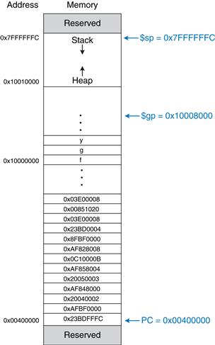
Figure 6.34 Executable loaded in memory
6.7 Odds and Ends*
This section covers a few optional topics that do not fit naturally elsewhere in the chapter. These topics include pseudoinstructions, exceptions, signed and unsigned arithmetic instructions, and floating-point instructions.
6.7.1 Pseudoinstructions
If an instruction is not available in the MIPS instruction set, it is probably because the same operation can be performed using one or more existing MIPS instructions. Remember that MIPS is a reduced instruction set computer (RISC), so the instruction size and hardware complexity are minimized by keeping the number of instructions small.
However, MIPS defines pseudoinstructions that are not actually part of the instruction set but are commonly used by programmers and compilers. When converted to machine code, pseudoinstructions are translated into one or more MIPS instructions.
Table 6.5 gives examples of pseudoinstructions and the MIPS instructions used to implement them. For example, the load immediate pseudoinstruction (li) loads a 32-bit constant using a combination of lui and ori instructions. The no operation pseudoinstruction (nop, pronounced “no op”) performs no operation. The PC is incremented by 4 upon its execution. No other registers or memory values are altered. The machine code for the nop instruction is 0x00000000.
Table 6.5 Pseudoinstructions
| Pseudoinstruction | Corresponding MIPS Instructions |
| li $s0, 0x1234AA77 | lui $s0, 0x1234 ori $s0, 0xAA77 |
| clear $t0 | add $t0, $0, $0 |
| move $s2, $s1 | add $s2, $s1, $0 |
| nop | sll $0, $0, 0 |
Some pseudoinstructions require a temporary register for intermediate calculations. For example, the pseudoinstruction beq $t2, imm15:0, Loop compares $t2 to a 16-bit immediate, imm15:0. This pseudoinstruction requires a temporary register in which to store the 16-bit immediate. Assemblers use the assembler register, $at, for such purposes. Table 6.6 shows how the assembler uses $at in converting a pseudoinstruction to real MIPS instructions. We leave it as Exercises 6.38 and 6.39 to implement other pseudoinstructions such as rotate left (rol) and rotate right (ror).
Table 6.6 Pseudoinstruction using $at
| Pseudoinstruction | Corresponding MIPS Instructions |
| beq $t2, imm15:0, Loop | addi $at, $0, imm15:0 beq$t2, $at, Loop |
6.7.2 Exceptions
An exception is like an unscheduled function call that jumps to a new address. Exceptions may be caused by hardware or software. For example, the processor may receive notification that the user pressed a key on a keyboard. The processor may stop what it is doing, determine which key was pressed, save it for future reference, then resume the program that was running. Such a hardware exception triggered by an input/output (I/O) device such as a keyboard is often called an interrupt. Alternatively, the program may encounter an error condition such as an undefined instruction. The program then jumps to code in the operating system (OS), which may choose to terminate the offending program. Software exceptions are sometimes called traps. Other causes of exceptions include division by zero, attempts to read nonexistent memory, hardware malfunctions, debugger breakpoints, and arithmetic overflow (see Section 6.7.3).
The processor records the cause of an exception and the value of the PC at the time the exception occurs. It then jumps to the exception handler function. The exception handler is code (usually in the OS) that examines the cause of the exception and responds appropriately (by reading the keyboard on a hardware interrupt, for example). It then returns to the program that was executing before the exception took place. In MIPS, the exception handler is always located at 0x80000180. When an exception occurs, the processor always jumps to this instruction address, regardless of the cause.
The MIPS architecture uses a special-purpose register, called the Cause register, to record the cause of the exception. Different codes are used to record different exception causes, as given in Table 6.7. The exception handler code reads the Cause register to determine how to handle the exception. Some other architectures jump to a different exception handler for each different cause instead of using a Cause register.
Table 6.7 Exception cause codes
| Exception | Cause |
| hardware interrupt | 0x00000000 |
| system call | 0x00000020 |
| breakpoint/divide by 0 | 0x00000024 |
| undefined instruction | 0x00000028 |
| arithmetic overflow | 0x00000030 |
MIPS uses another special-purpose register called the Exception Program Counter (EPC) to store the value of the PC at the time an exception takes place. The processor returns to the address in EPC after handling the exception. This is analogous to using $ra to store the old value of the PC during a jal instruction.
The EPC and Cause registers are not part of the MIPS register file. The mfc0 (move from coprocessor 0) instruction copies these and other special-purpose registers into one of the general purpose registers. Coprocessor 0 is called the MIPS processor control; it handles interrupts and processor diagnostics. For example, mfc0 $t0, Cause copies the Cause register into $t0.
The syscall and break instructions cause traps to perform system calls or debugger breakpoints. The exception handler uses the EPC to look up the instruction and determine the nature of the system call or breakpoint by looking at the fields of the instruction.
$k0 and $kl are included in the MIPS register set. They are reserved by the OS for exception handling. They do not need to be saved and restored during exceptions.
In summary, an exception causes the processor to jump to the exception handler. The exception handler saves registers on the stack, then uses mfc0 to look at the cause and respond accordingly. When the handler is finished, it restores the registers from the stack, copies the return address from EPC to $k0 using mfc0, and returns using jr $k0.
6.7.3 Signed and Unsigned Instructions
Recall that a binary number may be signed or unsigned. The MIPS architecture uses two’s complement representation of signed numbers. MIPS has certain instructions that come in signed and unsigned flavors, including addition and subtraction, multiplication and division, set less than, and partial word loads.
Addition and Subtraction
Addition and subtraction are performed identically whether the number is signed or unsigned. However, the interpretation of the results is different.
As mentioned in Section 1.4.6, if two large signed numbers are added together, the result may incorrectly produce the opposite sign. For example, adding the following two huge positive numbers gives a negative result: 0x7FFFFFFF + 0x7FFFFFFF = 0xFFFFFFFE = −2. Similarly, adding two huge negative numbers gives a positive result, 0x80000001 + 0x80000001 = 0x00000002. This is called arithmetic overflow.
The C language ignores arithmetic overflows, but other languages, such as Fortran, require that the program be notified. As mentioned in Section 6.7.2, the MIPS processor takes an exception on arithmetic overflow. The program can decide what to do about the overflow (for example, it might repeat the calculation with greater precision to avoid the overflow), then return to where it left off.
MIPS provides signed and unsigned versions of addition and subtraction. The signed versions are add, addi, and sub. The unsigned versions are addu, addiu, and subu. The two versions are identical except that signed versions trigger an exception on overflow, whereas unsigned versions do not. Because C ignores exceptions, C programs technically use the unsigned versions of these instructions.
Multiplication and Division
Multiplication and division behave differently for signed and unsigned numbers. For example, as an unsigned number, 0xFFFFFFFF represents a large number, but as a signed number it represents –1. Hence, 0xFFFFFFFF × 0xFFFFFFFF would equal 0xFFFFFFFE00000001 if the numbers were unsigned but 0x0000000000000001 if the numbers were signed.
Therefore, multiplication and division come in both signed and unsigned flavors. mult and div treat the operands as signed numbers. multu and divu treat the operands as unsigned numbers.
Set Less Than
Set less than instructions can compare either two registers (slt) or a register and an immediate (slti). Set less than also comes in signed (slt and slti) and unsigned (sltu and sltiu) versions. In a signed comparison, 0x80000000 is less than any other number, because it is the most negative two’s complement number. In an unsigned comparison, 0x80000000 is greater than 0x7FFFFFFF but less than 0x80000001, because all numbers are positive.
Beware that sltiu sign-extends the immediate before treating it as an unsigned number. For example, sltiu $s0, $s1, 0x8042 compares $s1 to 0xFFFF8042, treating the immediate as a large positive number.
Loads
As described in Section 6.4.5, byte loads come in signed (lb) and unsigned (lbu) versions. lb sign-extends the byte, and lbu zero-extends the byte to fill the entire 32-bit register. Similarly, MIPS provides signed and unsigned half-word loads (lh and lhu), which load two bytes into the lower half and sign- or zero-extend the upper half of the word.
6.7.4 Floating-Point Instructions
The MIPS architecture defines an optional floating-point coprocessor, known as coprocessor 1. In early MIPS implementations, the floating-point coprocessor was a separate chip that users could purchase if they needed fast floating-point math. In most recent MIPS implementations, the floating-point coprocessor is built in alongside the main processor.
MIPS defines thirty-two 32-bit floating-point registers, $f0–$f31. These are separate from the ordinary registers used so far. MIPS supports both single- and double-precision IEEE floating-point arithmetic. Double-precision (64-bit) numbers are stored in pairs of 32-bit registers, so only the 16 even-numbered registers ($f0, $f2, $f4, … , $f30) are used to specify double-precision operations. By convention, certain registers are reserved for certain purposes, as given in Table 6.8.
Table 6.8 MIPS floating-point register set
| Name | Number | Use |
| $fv0–$fv1 | 0, 2 | function return value |
| $ft0–$ft3 | 4, 6, 8, 10 | temporary variables |
| $fa0–$fa1 | 12, 14 | function arguments |
| $ft4–$ft5 | 16, 18 | temporary variables |
| $fs0–$fs5 | 20, 22, 24, 26, 28, 30 | saved variables |
Floating-point instructions all have an opcode of 17 (100012). They require both a funct field and a cop (coprocessor) field to indicate the type of instruction. Hence, MIPS defines the F-type instruction format for floating-point instructions, shown in Figure 6.35. Floating-point instructions come in both single- and double-precision flavors. cop = 16 (100002) for single-precision instructions or 17 (100012) for double-precision instructions. Like R-type instructions, F-type instructions have two source operands, fs and ft, and one destination, fd.

Figure 6.35 F-type machine instruction format
Instruction precision is indicated by .s and .d in the mnemonic. Floating-point arithmetic instructions include addition (add.s, add.d), subtraction (sub.s, sub.d), multiplication (mul.s, mul.d), and division (div.s, div.d) as well as negation (neg.s, neg.d) and absolute value (abs.s, abs.d).
Floating-point branches have two parts. First, a compare instruction is used to set or clear the floating-point condition flag (fpcond). Then, a conditional branch checks the value of the flag. The compare instructions include equality (c.seq.s/c.seq.d), less than (c.lt.s/c.lt.d), and less than or equal to (c.le.s/c.le.d). The conditional branch instructions are bc1f and bc1t that branch if fpcond is FALSE or TRUE, respectively. Inequality, greater than or equal to, and greater than comparisons are performed with seq, lt, and le, followed by bc1f.
Floating-point registers are loaded and stored from memory using lwc1 and swc1. These instructions move 32 bits, so two are necessary to handle a double-precision number.
6.8 Real-World Perspective: x86 Architecture*
Almost all personal computers today use x86 architecture microprocessors. x86, also called IA-32, is a 32-bit architecture originally developed by Intel. AMD also sells x86 compatible microprocessors.
The x86 architecture has a long and convoluted history dating back to 1978, when Intel announced the 16-bit 8086 microprocessor. IBM selected the 8086 and its cousin, the 8088, for IBM’s first personal computers. In 1985, Intel introduced the 32-bit 80386 microprocessor, which was backward compatible with the 8086, so it could run software developed for earlier PCs. Processor architectures compatible with the 80386 are called x86 processors. The Pentium, Core, and Athlon processors are well known x86 processors. Section 7.9 describes the evolution of x86 microprocessors in more detail.
Various groups at Intel and AMD over many years have shoehorned more instructions and capabilities into the antiquated architecture. The result is far less elegant than MIPS. As Patterson and Hennessy explain, “this checkered ancestry has led to an architecture that is difficult to explain and impossible to love.” However, software compatibility is far more important than technical elegance, so x86 has been the de facto PC standard for more than two decades. More than 100 million x86 processors are sold every year. This huge market justifies more than $5 billion of research and development annually to continue improving the processors.
x86 is an example of a Complex Instruction Set Computer (CISC) architecture. In contrast to RISC architectures such as MIPS, each CISC instruction can do more work. Programs for CISC architectures usually require fewer instructions. The instruction encodings were selected to be more compact, so as to save memory, when RAM was far more expensive than it is today; instructions are of variable length and are often less than 32 bits. The trade-off is that complicated instructions are more difficult to decode and tend to execute more slowly.
This section introduces the x86 architecture. The goal is not to make you into an x86 assembly language programmer, but rather to illustrate some of the similarities and differences between x86 and MIPS. We think it is interesting to see how x86 works. However, none of the material in this section is needed to understand the rest of the book. Major differences between x86 and MIPS are summarized in Table 6.9.
Table 6.9 Major differences between MIPS and x86
| Feature | MIPS | x86 |
| # of registers | 32 general purpose | 8, some restrictions on purpose |
| # of operands | 3 (2 source, 1 destination) | 2 (1 source, 1 source/destination) |
| operand location | registers or immediates | registers, immediates, or memory |
| operand size | 32 bits | 8, 16, or 32 bits |
| condition codes | no | yes |
| instruction types | simple | simple and complicated |
| instruction encoding | fixed, 4 bytes | variable, 1–15 bytes |
6.8.1 x86 Registers
The 8086 microprocessor provided eight 16-bit registers. It could separately access the upper and lower eight bits of some of these registers. When the 32-bit 80386 was introduced, the registers were extended to 32 bits. These registers are called EAX, ECX, EDX, EBX, ESP, EBP, ESI, and EDI. For backward compatibility, the bottom 16 bits and some of the bottom 8-bit portions are also usable, as shown in Figure 6.36.
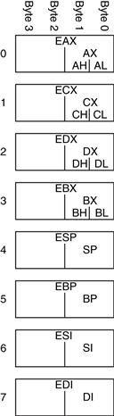
Figure 6.36 x86 registers
The eight registers are almost, but not quite, general purpose. Certain instructions cannot use certain registers. Other instructions always put their results in certain registers. Like $sp in MIPS, ESP is normally reserved for the stack pointer.
The x86 program counter is called EIP (the extended instruction pointer). Like the MIPS PC, it advances from one instruction to the next or can be changed with branch, jump, and function call instructions.
6.8.2 x86 Operands
MIPS instructions always act on registers or immediates. Explicit load and store instructions are needed to move data between memory and the registers. In contrast, x86 instructions may operate on registers, immediates, or memory. This partially compensates for the small set of registers.
MIPS instructions generally specify three operands: two sources and one destination. x86 instructions specify only two operands. The first is a source. The second is both a source and the destination. Hence, x86 instructions always overwrite one of their sources with the result. Table 6.10 lists the combinations of operand locations in x86. All combinations are possible except memory to memory.
Table 6.10 Operand locations
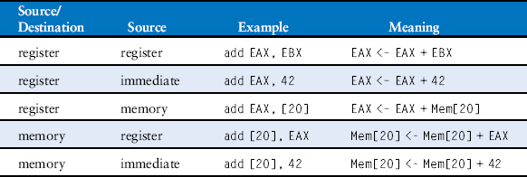
Like MIPS, x86 has a 32-bit memory space that is byte-addressable. However, x86 also supports a much wider variety of memory addressing modes. Memory locations are specified with any combination of a base register, displacement, and a scaled index register. Table 6.11 illustrates these combinations. The displacement can be an 8-, 16-, or 32-bit value. The scale multiplying the index register can be 1, 2, 4, or 8. The base + displacement mode is equivalent to the MIPS base addressing mode for loads and stores. The scaled index provides an easy way to access arrays or structures of 2-, 4-, or 8-byte elements without having to issue a sequence of instructions to generate the address.
Table 6.11 Memory addressing modes
| Example | Meaning | Comment |
| add EAX, [20] | EAX <– EAX + Mem[20] | displacement |
| add EAX, [ESP] | EAX <– EAX + Mem[ESP] | base addressing |
| add EAX, [EDX+40] | EAX <– EAX + Mem[EDX+40] | base + displacement |
| add EAX, [60+EDI*4] | EAX <– EAX + Mem[60+EDI*4] | displacement + scaled index |
| add EAX, [EDX+80+EDI*2] | EAX <– EAX + Mem[EDX+80+EDI*2] | base + displacement + scaled index |
While MIPS always acts on 32-bit words, x86 instructions can operate on 8-, 16-, or 32-bit data. Table 6.12 illustrates these variations.
Table 6.12 Instructions acting on 8-, 16-, or 32-bit data
| Example | Meaning | Data Size |
| add AH, BL | AH <– AH + BL | 8-bit |
| add AX, −1 | AX <– AX + 0xFFFF | 16-bit |
| add EAX, EDX | EAX <– EAX + EDX | 32-bit |
6.8.3 Status Flags
x86, like many CISC architectures, uses status flags (also called condition codes) to make decisions about branches and to keep track of carries and arithmetic overflow. x86 uses a 32-bit register, called EFLAGS, that stores the status flags. Some of the bits of the EFLAGS register are given in Table 6.13. Other bits are used by the operating system.
Table 6.13 Selected EFLAGS
| Name | Meaning |
| CF (Carry Flag) | Carry out generated by last arithmetic operation. Indicates overflow in unsigned arithmetic. Also used for propagating the carry between words in multiple-precision arithmetic. |
| ZF (Zero Flag) | Result of last operation was zero. |
| SF (Sign Flag) | Result of last operation was negative (msb = 1). |
| OF (Overflow Flag) | Overflow of two’s complement arithmetic. |
The architectural state of an x86 processor includes EFLAGS as well as the eight registers and the EIP.
6.8.4 x86 Instructions
x86 has a larger set of instructions than MIPS. Table 6.14 describes some of the general purpose instructions. x86 also has instructions for floating-point arithmetic and for arithmetic on multiple short data elements packed into a longer word. D indicates the destination (a register or memory location), and S indicates the source (a register, memory location, or immediate).
Table 6.14 Selected x86 instructions
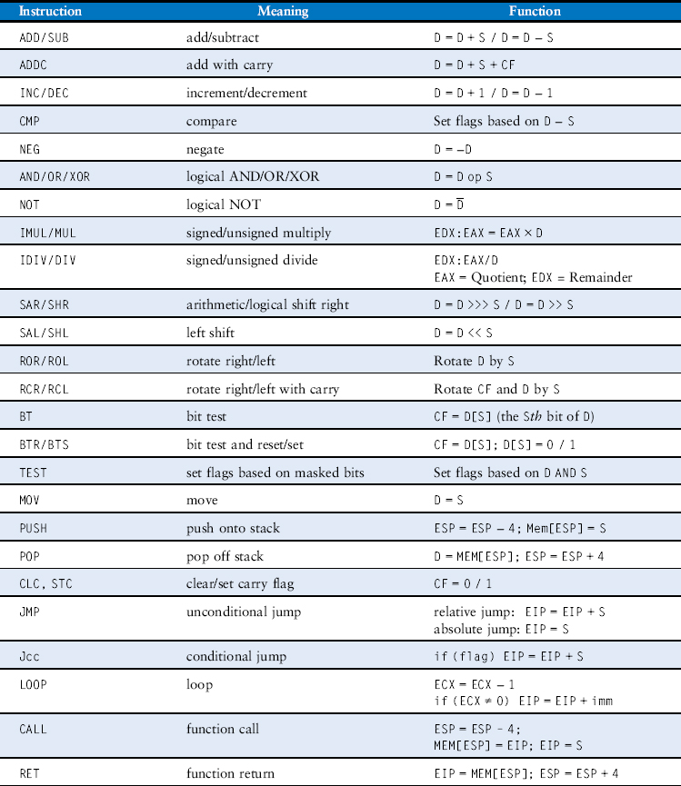
Note that some instructions always act on specific registers. For example, 32 × 32-bit multiplication always takes one of the sources from EAX and always puts the 64-bit result in EDX and EAX. LOOP always stores the loop counter in ECX. PUSH, POP, CALL, and RET use the stack pointer, ESP.
Conditional jumps check the flags and branch if the appropriate condition is met. They come in many flavors. For example, JZ jumps if the zero flag (ZF) is 1. JNZ jumps if the zero flag is 0. The jumps usually follow an instruction, such as the compare instruction (CMP), that sets the flags. Table 6.15 lists some of the conditional jumps and how they depend on the flags set by a prior compare operation.
Table 6.15 Selected branch conditions
| Instruction | Meaning | Function After CMP D, S |
| JZ/JE | jump if ZF = 1 | jump if D = S |
| JNZ/JNE | jump if ZF = 0 | jump if D ≠ S |
| JGE | jump if SF = OF | jump if D ≥ S |
| JG | jump if SF = OF and ZF = 0 | jump if D > S |
| JLE | jump if SF ≠ OF or ZF = 1 | jump if D ≤ S |
| JL | jump if SF ≠ OF | jump if D < S |
| JC/JB | jump if CF = 1 | |
| JNC | jump if CF = 0 | |
| JO | jump if OF = 1 | |
| JNO | jump if OF = 0 | |
| JS | jump if SF = 1 | |
| JNS | jump if SF = 0 |
6.8.5 x86 Instruction Encoding
The x86 instruction encodings are truly messy, a legacy of decades of piecemeal changes. Unlike MIPS, whose instructions are uniformly 32 bits, x86 instructions vary from 1 to 15 bytes, as shown in Figure 6.37.3 The opcode may be 1, 2, or 3 bytes. It is followed by four optional fields: Mod R/M, SIB, Displacement, and Immediate. ModR/M specifies an addressing mode. SIB specifies the scale, index, and base registers in certain addressing modes. Displacement indicates a 1-, 2-, or 4-byte displacement in certain addressing modes. And Immediate is a 1-, 2-, or 4-byte constant for instructions using an immediate as the source operand. Moreover, an instruction can be preceded by up to four optional byte-long prefixes that modify its behavior.
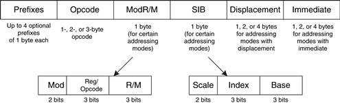
Figure 6.37 x86 instruction encodings
The ModR/M byte uses the 2-bit Mod and 3-bit R/M field to specify the addressing mode for one of the operands. The operand can come from one of the eight registers, or from one of 24 memory addressing modes. Due to artifacts in the encodings, the ESP and EBP registers are not available for use as the base or index register in certain addressing modes. The Reg field specifies the register used as the other operand. For certain instructions that do not require a second operand, the Reg field is used to specify three more bits of the opcode.
In addressing modes using a scaled index register, the SIB byte specifies the index register and the scale (1, 2, 4, or 8). If both a base and index are used, the SIB byte also specifies the base register.
MIPS fully specifies the instruction in the opcode and funct fields of the instruction. x86 uses a variable number of bits to specify different instructions. It uses fewer bits to specify more common instructions, decreasing the average length of the instructions. Some instructions even have multiple opcodes. For example, add AL, imm8 performs an 8-bit add of an immediate to AL. It is represented with the 1-byte opcode, 0x04, followed by a 1-byte immediate. The A register (AL, AX, or EAX) is called the accumulator. On the other hand, add D, imm8 performs an 8-bit add of an immediate to an arbitrary destination, D (memory or a register). It is represented with the 1-byte opcode 0x80 followed by one or more bytes specifying D, followed by a 1-byte immediate. Many instructions have shortened encodings when the destination is the accumulator.
In the original 8086, the opcode specified whether the instruction acted on 8- or 16-bit operands. When the 80386 introduced 32-bit operands, no new opcodes were available to specify the 32-bit form. Instead, the same opcode was used for both 16- and 32-bit forms. An additional bit in the code segment descriptor used by the OS specifies which form the processor should choose. The bit is set to 0 for backward compatibility with 8086 programs, defaulting the opcode to 16-bit operands. It is set to 1 for programs to default to 32-bit operands. Moreover, the programmer can specify prefixes to change the form for a particular instruction. If the prefix 0x66 appears before the opcode, the alternative size operand is used (16 bits in 32-bit mode, or 32 bits in 16-bit mode).
6.8.6 Other x86 Peculiarities
The 80286 introduced segmentation to divide memory into segments of up to 64 KB in length. When the OS enables segmentation, addresses are computed relative to the beginning of the segment. The processor checks for addresses that go beyond the end of the segment and indicates an error, thus preventing programs from accessing memory outside their own segment. Segmentation proved to be a hassle for programmers and is not used in modern versions of the Windows operating system.
x86 contains string instructions that act on entire strings of bytes or words. The operations include moving, comparing, or scanning for a specific value. In modern processors, these instructions are usually slower than performing the equivalent operation with a series of simpler instructions, so they are best avoided.
As mentioned earlier, the 0x66 prefix is used to choose between 16- and 32-bit operand sizes. Other prefixes include ones used to lock the bus (to control access to shared variables in a multiprocessor system), to predict whether a branch will be taken or not, and to repeat the instruction during a string move.
Intel and Hewlett-Packard jointly developed a new 64-bit architecture called IA-64 in the mid 1990’s. It was designed from a clean slate, bypassing the convoluted history of x86, taking advantage of 20 years of new research in computer architecture, and providing a 64-bit address space. However, IA-64 has yet to become a market success. Most computers needing the large address space now use the 64-bit extensions of x86.
The bane of any architecture is to run out of memory capacity. With 32-bit addresses, x86 can access 4 GB of memory. This was far more than the largest computers had in 1985, but by the early 2000s it had become limiting. In 2003, AMD extended the address space and register sizes to 64 bits, calling the enhanced architecture AMD64. AMD64 has a compatibility mode that allows it to run 32-bit programs unmodified while the OS takes advantage of the bigger address space. In 2004, Intel gave in and adopted the 64-bit extensions, renaming them Extended Memory 64 Technology (EM64T). With 64-bit addresses, computers can access 16 exabytes (16 billion GB) of memory.
For those curious about more details of the x86 architecture, the x86 Intel Architecture Software Developer’s Manual is freely available on Intel’s Web site.
6.8.7 The Big Picture
This section has given a taste of some of the differences between the MIPS RISC architecture and the x86 CISC architecture. x86 tends to have shorter programs, because a complex instruction is equivalent to a series of simple MIPS instructions and because the instructions are encoded to minimize memory use. However, the x86 architecture is a hodgepodge of features accumulated over the years, some of which are no longer useful but must be kept for compatibility with old programs. It has too few registers, and the instructions are difficult to decode. Merely explaining the instruction set is difficult. Despite all these failings, x86 is firmly entrenched as the dominant computer architecture for PCs, because the value of software compatibility is so great and because the huge market justifies the effort required to build fast x86 microprocessors.
6.9 Summary
To command a computer, you must speak its language. A computer architecture defines how to command a processor. Many different computer architectures are in widespread commercial use today, but once you understand one, learning others is much easier. The key questions to ask when approaching a new architecture are
MIPS is a 32-bit architecture because it operates on 32-bit data. The MIPS architecture has 32 general-purpose registers. In principle, almost any register can be used for any purpose. However, by convention, certain registers are reserved for certain purposes, for ease of programming and so that functions written by different programmers can communicate easily. For example, register 0 ($0) always holds the constant 0, $ra holds the return address after a jal instruction, and $a0–$a3 and $v0–$v1 hold the arguments and return value of a function. MIPS has a byte-addressable memory system with 32-bit addresses. The memory map was described in Section 6.6.1. Instructions are 32 bits long and must be word aligned. This chapter discussed the most commonly used MIPS instructions.
The power of defining a computer architecture is that a program written for any given architecture can run on many different implementations of that architecture. For example, programs written for the Intel Pentium processor in 1993 will generally still run (and run much faster) on the Intel Xeon or AMD Phenom processors in 2012.
In the first part of this book, we learned about the circuit and logic levels of abstraction. In this chapter, we jumped up to the architecture level. In the next chapter, we study microarchitecture, the arrangement of digital building blocks that implement a processor architecture. Microarchitecture is the link between hardware and software engineering. And, we believe it is one of the most exciting topics in all of engineering: you will learn to build your own microprocessor!
Exercises
Exercise 6.1 Give three examples from the MIPS architecture of each of the architecture design principles: (1) simplicity favors regularity; (2) make the common case fast; (3) smaller is faster; and (4) good design demands good compromises. Explain how each of your examples exhibits the design principle.
Exercise 6.2 The MIPS architecture has a register set that consists of 32-bit registers. Is it possible to design a computer architecture without a register set? If so, briefly describe the architecture, including the instruction set. What are advantages and disadvantages of this architecture over the MIPS architecture?
Exercise 6.3 Consider memory storage of a 32-bit word stored at memory word 42 in a byte-addressable memory.
(a) What is the byte address of memory word 42?
(b) What are the byte addresses that memory word 42 spans?
(c) Draw the number 0xFF223344 stored at word 42 in both big-endian and little-endian machines. Your drawing should be similar to Figure 6.4. Clearly label the byte address corresponding to each data byte value.
Exercise 6.4 Repeat Exercise 6.3 for memory storage of a 32-bit word stored at memory word 15 in a byte-addressable memory.
Exercise 6.5 Explain how the following program can be used to determine whether a computer is big-endian or little-endian:
li $t0, 0xABCD9876
sw $t0, 100($0)
lb $s5, 101($0)
Exercise 6.6 Write the following strings using ASCII encoding. Write your final answers in hexadecimal.
Exercise 6.7 Repeat Exercise 6.6 for the following strings.
Exercise 6.8 Show how the strings in Exercise 6.6 are stored in a byte-addressable memory on (a) a big-endian machine and (b) a little-endian machine starting at memory address 0x1000100C. Use a memory diagram similar to Figure 6.4. Clearly indicate the memory address of each byte on each machine.
Exercise 6.9 Repeat Exercise 6.8 for the strings in Exercise 6.7.
Exercise 6.10 Convert the following MIPS assembly code into machine language. Write the instructions in hexadecimal.
add $t0, $s0, $s1
lw $t0, 0x20($t7)
addi $s0, $0, −10
Exercise 6.11 Repeat Exercise 6.10 for the following MIPS assembly code:
addi $s0, $0, 73
sw $t1, −7($t2)
sub $t1, $s7, $s2
Exercise 6.12 Consider I-type instructions.
(a) Which instructions from Exercise 6.10 are I-type instructions?
(b) Sign-extend the 16-bit immediate of each instruction from part (a) so that it becomes a 32-bit number.
Exercise 6.13 Repeat Exercise 6.12 for the instructions in Exercise 6.11.
Exercise 6.14 Convert the following program from machine language into MIPS assembly language. The numbers on the left are the instruction addresses in memory, and the numbers on the right give the instruction at that address. Then reverse engineer a high-level program that would compile into this assembly language routine and write it. Explain in words what the program does. $a0 is the input, and it initially contains a positive number, n. $v0 is the output.
0x00400000 0x20080000
0x00400004 0x20090001
0x00400008 0x0089502A
0x0040000C 0x15400003
0x00400010 0x01094020
0x00400014 0x21290002
0x00400018 0x08100002
0x0040001C 0x01001020
0x00400020 0x03E00008
Exercise 6.15 Repeat Exercise 6.14 for the following machine code. $a0 and $a1 are the inputs. $a0 contains a 32-bit number and $a1 is the address of a 32-element array of characters (char).
0x00400000 0x2008001F
0x00400004 0x01044806
0x00400008 0x31290001
0x0040000C 0x0009482A
0x00400010 0xA0A90000
0x00400014 0x20A50001
0x00400018 0x2108FFFF
0x0040001C 0x0501FFF9
0x00400020 0x03E00008
Exercise 6.16 The nori instruction is not part of the MIPS instruction set, because the same functionality can be implemented using existing instructions. Write a short assembly code snippet that has the following functionality: $t0 = $t1 NOR 0xF234. Use as few instructions as possible.
Exercise 6.17 Implement the following high-level code segments using the slt instruction. Assume the integer variables g and h are in registers $s0 and $s1, respectively.
Exercise 6.18 Write a function in a high-level language for int find42(int array[], int size). size specifies the number of elements in array, and array specifies the base address of the array. The function should return the index number of the first array entry that holds the value 42. If no array entry is 42, it should return the value –1.
Exercise 6.19 The high-level function strcpy copies the character string src to the character string dst (see page 360).
This simple string copy function has a serious flaw: it has no way of knowing that dst has enough space to receive src. If a malicious programmer were able to execute strcpy with a long string src, the programmer might be able to write bytes all over memory, possibly even modifying code stored in subsequent memory locations. With some cleverness, the modified code might take over the machine. This is called a buffer overflow attack; it is employed by several nasty programs, including the infamous Blaster worm, which caused an estimated $525 million in damages in 2003.
// C code
void strcpy(char dst[], char src[]) {
int i = 0;
do {
dst[i] = src[i];
} while (src[i++]);
}
(a) Implement the strcpy function in MIPS assembly code. Use $s0 for i.
(b) Draw a picture of the stack before, during, and after the strcpy function call. Assume $sp = 0x7FFFFF00 just before strcpy is called.
Exercise 6.20 Convert the high-level function from Exercise 6.18 into MIPS assembly code.
Exercise 6.21 Consider the MIPS assembly code below. func1, func2, and func3 are non-leaf functions. func4 is a leaf function. The code is not shown for each function, but the comments indicate which registers are used within each function.
0x00401000 func1 : … # func1 uses $s0–$s1
0x00401020 jal func2
…
0x00401100 func2: … # func2 uses $s2–$s7
0x0040117C jal func3
…
0x00401400 func3: … # func3 uses $s1–$s3
0x00401704 jal func4
…
0x00403008 func4: … # func4 uses no preserved
0x00403118 jr $ra # registers
(a) How many words are the stack frames of each function?
(b) Sketch the stack after func4 is called. Clearly indicate which registers are stored where on the stack and mark each of the stack frames. Give values where possible.
Exercise 6.22 Each number in the Fibonacci series is the sum of the previous two numbers. Table 6.16 lists the first few numbers in the series, fib(n).
Table 6.16 Fibonacci series

(a) What is fib(n) for n = 0 and n = –1?
(b) Write a function called fib in a high-level language that returns the Fibonacci number for any nonnegative value of n. Hint: You probably will want to use a loop. Clearly comment your code.
(c) Convert the high-level function of part (b) into MIPS assembly code. Add comments after every line of code that explain clearly what it does. Use the SPIM simulator to test your code on fib(9). (See the Preface for how to install the SPIM simulator.)
Exercise 6.23 Consider C Code Example 6.27. For this exercise, assume factorial is called with input argument n = 5.
(a) What value is in $v0 when factorial returns to the calling function?
(b) Suppose you delete the instructions at addresses 0x98 and 0xBC that save and restore $ra. Will the program (1) enter an infinite loop but not crash; (2) crash (cause the stack to grow beyond the dynamic data segment or the PC to jump to a location outside the program); (3) produce an incorrect value in $v0 when the program returns to loop (if so, what value?), or (4) run correctly despite the deleted lines?
(c) Repeat part (b) when the instructions at the following instruction addresses are deleted:
(i) 0x94 and 0xC0 (instructions that save and restore $a0)
(ii) 0x90 and 0xC4 (instructions that save and restore $sp). Note: the factorial label is not deleted
Exercise 6.24 Ben Bitdiddle is trying to compute the function f(a, b) = 2a + 3b for nonnegative b. He goes overboard in the use of function calls and recursion and produces the following high-level code for functions f and f2.
// high-level code for functions f and f2
int f(int a, int b) {
int j;
j = a;
return j + a + f2(b);
}
int f2(int x)
{
int k;
k = 3;
if (x == 0) return 0;
else return k + f2(x − l);
}
Ben then translates the two functions into assembly language as follows. He also writes a function, test, that calls the function f(5, 3).
# MIPS assembly code
# f: $a0 = a, $a1 = b, $s0 = j; f2: $a0 = x, $s0 = k
0x00400000 test: addi $a0, $0, 5 # $a0 = 5 (a = 5)
0x00400004 addi $a1, $0, 3 # $a1 = 3 (b = 3)
0x00400008 jal f # call f(5, 3)
0x0040000C loop: j loop # and loop forever
0x00400010 f: addi $sp, $sp, −16 # make room on the stack
# for $s0, $a0, $a1, and $ra
0x00400014 sw $a1, 12($sp) # save $a1 (b)
0x00400018 sw $a0, 8($sp) # save $a0 (a)
0x0040001C sw $ra, 4($sp) # save $ra
0x00400020 sw $s0, 0($sp) # save $s0
0x00400024 add $s0, $a0, $0 # $s0 = $a0 (j = a)
0x00400028 add $a0, $a1, $0 # place b as argument for f2
0x0040002C jal f2 # call f2(b)
0x00400030 lw $a0, 8($sp) # restore $a0 (a) after call
0x00400034 lw $a1, 12($sp) # restore $a1 (b) after call
0x00400038 add $v0, $v0, $s0 # $v0 = f2(b) + j
0x0040003C add $v0, $v0, $a0 # $v0 = (f2(b) + j) + a
0x00400040 lw $s0, 0($sp) # restore $s0
0x00400044 lw $ra, 4($sp) # restore $ra
0x00400048 addi $sp, $sp, 16 # restore $sp (stack pointer)
0x0040004C jr $ra # return to point of call
0x00400050 f2: addi $sp, $sp, −12 # make room on the stack for
# $s0, $a0, and $ra
0x00400054 sw $a0, 8($sp) # save $a0 (x)
0x00400058 sw $ra, 4($sp) # save return address
0x0040005C sw $s0, 0($sp) # save $s0
0x00400060 addi $s0, $0, 3 # k = 3
0x00400064 bne $a0, $0, else # x = 0?
0x00400068 addi $v0, $0, 0 # yes: return value should be 0
0x0040006C j done # and clean up
0x00400070 else:addi $a0, $a0, −1 # no: $a0 = $a0 − 1 (x = x − 1)
0x00400074 jal f2 # call f2(x − 1)
0x00400078 lw $a0, 8($sp) # restore $a0 (x)
0x0040007C add $v0, $v0, $s0 # $v0 = f2(x − 1) + k
0x00400080 done: lw $s0, 0($sp) # restore $s0
0x00400084 lw $ra, 4($sp) # restore $ra
0x00400088 addi $sp, $sp, 12 # restore $sp
0x0040008C jr $ra # return to point of call
You will probably find it useful to make drawings of the stack similar to the one in Figure 6.26 to help you answer the following questions.
(a) If the code runs starting at test, what value is in $v0 when the program gets to loop? Does his program correctly compute 2a + 3b?
(b) Suppose Ben deletes the instructions at addresses 0x0040001C and 0x00400044 that save and restore $ra. Will the program (1) enter an infinite loop but not crash; (2) crash (cause the stack to grow beyond the dynamic data segment or the PC to jump to a location outside the program); (3) produce an incorrect value in $v0 when the program returns to loop (if so, what value?), or (4) run correctly despite the deleted lines?
(c) Repeat part (b) when the instructions at the following instruction addresses are deleted. Note that labels aren’t deleted, only instructions.
(i) 0x00400018 and 0x00400030 (instructions that save and restore $a0)
(ii) 0x00400014 and 0x00400034 (instructions that save and restore $a1)
(iii) 0x00400020 and 0x00400040 (instructions that save and restore $s0)
(iv) 0x00400050 and 0x00400088 (instructions that save and restore $sp)
(v) 0x0040005C and 0x00400080 (instructions that save and restore $s0)
(vi) 0x00400058 and 0x00400084 (instructions that save and restore $ra)
(vii) 0x00400054 and 0x00400078 (instructions that save and restore $a0)
Exercise 6.25 Convert the following beq, j, and jal assembly instructions into machine code. Instruction addresses are given to the left of each instruction.
(a) 0x00401000 beq $t0, $s1, Loop
0x00401004 …
0x00401008 …
0x0040100C Loop: …
(b) 0x00401000 beq $t7, $s4, done
… …
0x00402040 done: …
(c) 0x0040310C back: …
… …
0x00405000 beq $t9, $s7, back
Exercise 6.26 Consider the following MIPS assembly language snippet. The numbers to the left of each instruction indicate the instruction address.
0x00400028 add $a0, $a1, $0
0x0040002C jal f2
0x00400030 f1: jr $ra
0x00400034 f2: sw $s0, 0($s2)
0x00400038 bne $a0, $0, else
0x0040003C j f1
0x00400040 else: addi $a0, $a0, −1
0x00400044 j f2
(a) Translate the instruction sequence into machine code. Write the machine code instructions in hexadecimal.
Exercise 6.27 Consider the following C code snippet.
// C code
void setArray(int num) {
int i;
int array[10];
for (i = 0; i < 10; i = i + 1) {
array[i] = compare(num, i);
}
}
int compare(int a, int b) {
if (sub(a, b) >= 0)
return 1;
else
return 0;
}
int sub(int a, int b) {
return a − b;
}
(a) Implement the C code snippet in MIPS assembly language. Use $s0 to hold the variable i. Be sure to handle the stack pointer appropriately. The array is stored on the stack of the setArray function (see Section 6.4.6).
(b) Assume setArray is the first function called. Draw the status of the stack before calling setArray and during each function call. Indicate the names of registers and variables stored on the stack, mark the location of $sp, and clearly mark each stack frame.
(c) How would your code function if you failed to store $ra on the stack?
Exercise 6.28 Consider the following high-level function.
// C code
int f(int n, int k) {
int b;
b = k + 2;
if (n == 0) b = 10;
else b = b + (n * n) + f(n − 1, k + 1);
return b * k;
}
(a) Translate the high-level function f into MIPS assembly language. Pay particular attention to properly saving and restoring registers across function calls and using the MIPS preserved register conventions. Clearly comment your code. You can use the MIPS mul instruction. The function starts at instruction address 0x00400100. Keep local variable b in $s0.
(b) Step through your function from part (a) by hand for the case of f(2, 4). Draw a picture of the stack similar to the one in Figure 6.26(c). Write the register name and data value stored at each location in the stack and keep track of the stack pointer value ($sp). Clearly mark each stack frame. You might also find it useful to keep track of the values in $a0, $a1, $v0, and $s0 throughout execution. Assume that when f is called, $s0 = 0xABCD and $ra = 0x400004. What is the final value of $v0?
Exercise 6.29 What is the range of instruction addresses to which conditional branches, such as beq and bne, can branch in MIPS? Give your answer in number of instructions relative to the conditional branch instruction.
Exercise 6.30 The following questions examine the limitations of the jump instruction, j. Give your answer in number of instructions relative to the jump instruction.
(a) In the worst case, how far can the jump instruction (j) jump forward (i.e., to higher addresses)? (The worst case is when the jump instruction cannot jump far.) Explain using words and examples, as needed.
(b) In the best case, how far can the jump instruction (j) jump forward? (The best case is when the jump instruction can jump the farthest.) Explain.
(c) In the worst case, how far can the jump instruction (j) jump backward (to lower addresses)? Explain.
(d) In the best case, how far can the jump instruction (j) jump backward? Explain.
Exercise 6.31 Explain why it is advantageous to have a large address field, addr, in the machine format for the jump instructions, j and jal.
Exercise 6.32 Write assembly code that jumps to an instruction 64 Minstructions from the first instruction. Recall that 1 Minstruction = 220 instructions = 1,048,576 instructions. Assume that your code begins at address 0x00400000. Use a minimum number of instructions.
Exercise 6.33 Write a function in high-level code that takes a 10-entry array of 32-bit integers stored in little-endian format and converts it to big-endian format. After writing the high-level code, convert it to MIPS assembly code. Comment all your code and use a minimum number of instructions.
Exercise 6.34 Consider two strings: string1 and string2.
(a) Write high-level code for a function called concat that concatenates (joins together) the two strings: void concat(char string1[], char string2[], char stringconcat[]). The function does not return a value. It concatenates string1 and string2 and places the resulting string in stringconcat. You may assume that the character array stringconcat is large enough to accommodate the concatenated string.
(b) Convert the function from part (a) into MIPS assembly language.
Exercise 6.35 Write a MIPS assembly program that adds two positive single-precision floating point numbers held in $s0 and $s1. Do not use any of the MIPS floating-point instructions. You need not worry about any of the encodings that are reserved for special purposes (e.g., 0, NANs, etc.) or numbers that overflow or underflow. Use the SPIM simulator to test your code. You will need to manually set the values of $s0 and $s1 to test your code. Demonstrate that your code functions reliably.
Exercise 6.36 Show how the following MIPS program would be loaded into memory and executed.
# MIPS assembly code
main:
addi $sp, $sp, −4
sw $ra, 0($sp)
lw $a0, x
lw $a1, y
jal diff
lw $ra, 0($sp)
addi $sp, $sp, 4
jr $ra
diff:
sub $v0, $a0, $a1
jr $ra
(a) First show the instruction address next to each assembly instruction.
(b) Draw the symbol table showing the labels and their addresses.
(c) Convert all instructions into machine code.
(d) How big (how many bytes) are the data and text segments?
(e) Sketch a memory map showing where data and instructions are stored.
Exercise 6.37 Repeat Exercise 6.36 for the following MIPS code.
# MIPS assembly code
main:
addi $sp, $sp, −4
sw $ra, 0($sp)
addi $t0, $0, 15
sw $t0, a
addi $a1, $0, 27
sw $a1, b
lw $a0, a
jal greater
lw $ra, 0($sp)
addi $sp, $sp, 4
jr $ra
greater:
slt $v0, $a1, $a0
jr $ra
Exercise 6.38 Show the MIPS instructions that implement the following pseudoinstructions. You may use the assembler register, $at, but you may not corrupt (overwrite) any other registers.
(c) rol $t0, $t1, 5 (rotate $t1 left by 5 and put the result in $t0)
(d) ror $s4, $t6, 31 (rotate $t6 right by 31 and put the result in $s4)
Exercise 6.39 Repeat Exercise 6.38 for the following pseudoinstructions.
Interview Questions
The following exercises present questions that have been asked at interviews for digital design jobs (but are usually open to any assembly language).
Question 6.1 Write MIPS assembly code for swapping the contents of two registers, $t0 and $t1. You may not use any other registers.
Question 6.2 Suppose you are given an array of both positive and negative integers. Write MIPS assembly code that finds the subset of the array with the largest sum. Assume that the array’s base address and the number of array elements are in $a0 and $a1, respectively. Your code should place the resulting subset of the array starting at base address $a2. Write code that runs as fast as possible.
Question 6.3 You are given an array that holds a C string. The string forms a sentence. Design an algorithm for reversing the words in the sentence and storing the new sentence back in the array. Implement your algorithm using MIPS assembly code.
Question 6.4 Design an algorithm for counting the number of 1’s in a 32-bit number. Implement your algorithm using MIPS assembly code.
Question 6.5 Write MIPS assembly code to reverse the bits in a register. Use as few instructions as possible. Assume the register of interest is $t3.
Question 6.6 Write MIPS assembly code to test whether overflow occurs when $t2 and $t3 are added. Use a minimum number of instructions.
Question 6.7 Design an algorithm for testing whether a given string is a palindrome. (Recall that a palindrome is a word that is the same forward and backward. For example, the words “wow” and “racecar” are palindromes.) Implement your algorithm using MIPS assembly code.
1 SPIM, the MIPS simulator that comes with this text, uses the endianness of the machine it is run on. For example, when using SPIM on an Intel x86 machine, the memory is little-endian. With an older Macintosh or Sun SPARC machine, memory is big-endian.
2 In practice, because of pipelining (discussed in Chapter 7), MIPS processors have a branch delay slot. This means that the instruction immediately after a branch or jump is always executed. This idiosyncracy is ignored in MIPS assembly code in this chapter.
3 It is possible to construct 17-byte instructions if all the optional fields are used. However, x86 places a 15-byte limit on the length of legal instructions.