
In this recipe, we will look at a tried and tested technique for simulating ocean waves using a series of Gerstner waves at varying amplitudes, wave lengths, frequencies, and directions within a vertex shader (or domain shader).
For this recipe, we need to render a plane along the x and z axis. The completed solution uses an FBX scene with a simple subdivided mesh and UV coordinates for a normal map, however, a quad passed to the tessellation pipeline will also work; or better yet, a mesh generated in the vertex shader based on the SV_VertexID and SV_InstanceID input semantics.
A prerequisite is the mesh renderer and shaders that implement normal mapping as shown in the Adding surface detail with normal mapping recipe of Chapter 6, Adding Surface Detail with Normal and Displacement Mapping.
As we will be generating sine waves over a period of time, we need to add a Time property to our PerFrame constant buffer. Then we will implement the vertex displacement within a vertex shader. Consider the following steps:
- Within
Common.hlsl, update thePerFramestructure (as shown in the highlighted section of the following code):cbuffer PerFrame: register (b1) { DirectionalLight Light; float3 CameraPosition; float Time; }; - Within your
ConstantBuffers.csfile, update the matchingPerFramestructure to include the time component.[StructLayout(LayoutKind.Sequential, Pack = 1)] public struct PerFrame { public DirectionalLight Light; public SharpDX.Vector3 CameraPosition; public float Time; } - Within the render loop, update the code for setting up the
perFrameconstant buffer, by setting up theTimeproperty.perFrame.CameraPosition = cameraPosition; // Provide simulation time to shader perFrame.Time = (float)simTime.Elapsed.TotalSeconds; context.UpdateSubresource(ref perFrame, perFrameBuffer);
- Next, add the
SubdividedPlane.fbxto your project, set the Build Action to MeshContentTask, and load it into aMeshRendererinstance. Alternatively, if you are using the tessellation pipeline, create a quad with a width (X-axis) and depth (Z-axis) of around 24 units and a tessellation factor in the range of approximately 10.0 to 20.0.var loadedMesh = Common.Mesh.LoadFromFile("SubdividedPlane.cmo"); var waterMesh = ToDispose(new MeshRenderer(loadedMesh.First())); waterMesh.Initialize(this);Now, we can update the vertex shader to implement the displacement. If you are using the tessellation pipeline, the same changes will be made to your domain shader instead.
- First, we will add a new HLSL function to our vertex shader file in order to generate the waveform.
void GerstnerWaveTessendorf(float waveLength, float speed, float amplitude, float steepness, float2 direction, in float3 position, inout float3 result, inout float3 normal, inout float3 tangent) { ...SNIP see next steps } - Within the preceding function, we will initialize the values for the Gerstner formula as follows:
float L = waveLength;// wave crest to crest
float A = amplitude; // wave height
float k = 2.0 * 3.1416 / L; // wave length
float kA = k*A;
float2 D = normalize(direction); // normalized direction
float2 K = D * k; // wave vector and magnitude (direction)
// peak/crest steepness, higher means steeper, but too much
// can cause the wave to become inside out at the top
// A value of zero results in a sine wave.
float Q = steepness;

// Calculate wave speed (frequency) from input
float S = speed * 0.5; // Speed 1 =~ 2m/s so halve first
float w = S * k; // Phase/frequency
float wT = w * Time;

// Calculate values for reuse
float KPwT = dot(K, position.xz)-wT;
float S0 = sin(KPwT);
float C0 = cos(KPwT);
- Next, we will calculate the vertex offset from the provided direction and current vertex position.
// Calculate the vertex offset along the X and Z axes
float2 xz = position.xz - D*Q*A*S0;
// Calculate the vertex offset along the Y (up/down) axis
float y = A*C0;
- Then, we need to calculate the new normal and tangent vectors, as follows:
// Calculate the tangent/bitangent/normal // Bitangent float3 B = float3( 1-(Q * D.x * D.x * kA * C0), D.x * kA * S0, -(Q*D.x * D.y * kA * C0)); // Tangent float3 T = float3( -(Q * D.x * D.y * kA * C0), D.y * kA * S0, 1-(Q*D.y * D.y * kA * C0)); B = normalize(B); T = normalize(T); float3 N = cross(T, B); - And lastly, set the output values. Note that we are accumulating the results in order to call the method multiple times with varying parameters.
// Append the results
result.xz += xz;
result.y += y;
normal += N;
tangent += T;
With the Gerstner wave function in place, we can now displace the vertices within our vertex or domain shader.
- The following is an example of the code that is necessary to generate gentle ocean waves. This should be inserted before any
WorldViewProjectionorViewProjectiontransforms....SNIP // Existing vertex shader code float3 N = (float3)0; // normal float3 T = (float3)0; // tangent float3 waveOffset = (float3)0; // vertex xyz offset float2 direction = float2(1, 0); // Gentle ocean waves GerstnerWaveTessendorf(8, 0.5, 0.3, 1, direction, vertex.Position, waveOffset, N, T); GerstnerWaveTessendorf(4, 0.5, 0.4, 1, direction + float2(0, 0.5), vertex.Position, waveOffset, N, T); GerstnerWaveTessendorf(3, 0.5, 0.3, 1, direction + float2(0, 1), vertex.Position, waveOffset, N, T); GerstnerWaveTessendorf(2.5, 0.5, 0.2, 1, direction, vertex.Position, waveOffset, N, T); vertex.Position.xyz += waveOffset; vertex.Normal = normalize(N); vertex.Tangent.xyz = normalize(T); // If using normal mapping // Existing vertex shader code result.Position = mul(vertex.Position, WorldViewProjection); ...SNIP - For larger and more choppy waves, you can try the following code instead:
// Choppy ocean waves
GerstnerWaveTessendorf(10, 2, 2.5, 0.5, direction, vertex.Position, waveOffset, N, T);
GerstnerWaveTessendorf(5, 1.2, 2, 1, direction, vertex.Position, waveOffset, N, T);
GerstnerWaveTessendorf(4, 2, 2, 1, direction + float2(0, 1), vertex.Position, waveOffset, N, T);
GerstnerWaveTessendorf(4, 1, 0.5, 1, direction + float2(0, 1), vertex.Position, waveOffset, N, T);
GerstnerWaveTessendorf(2.5, 2, 0.5, 1, direction + float2(0, 0.5), vertex.Position, waveOffset, N, T);
GerstnerWaveTessendorf(2, 2, 0.5, 1, direction, vertex.Position, waveOffset, N, T);
This completes our HLSL shader code.
- Now, render the mesh within your render loop, and ensure that the correct vertex shader is assigned (if a new shader has been created, compile it within the appropriate location).
// If showing normal map
waterMesh.DisableNormalMap = disableNormalMap;
waterMesh.PerMaterialBuffer = perMaterialBuffer;
waterMesh.PerArmatureBuffer = perArmatureBuffer;
waterMesh.Render();
The completed project in the downloadable companion code maps the Backspace key to switch between the previous physics scene and this recipe. Pressing Shift + N toggles between the diffuse mapping as well as the diffuse and normal mapping, and the N key will toggle the display of the debug normal vectors. The final result of the gentle and choppy waves, is shown in the following diagram:

Multiple Gerstner waves: gentle ocean waves (left), choppy ocean waves (right), wireframe (top) with debug normal vectors (top-left), diffuse shader (middle), and diffuse + normal mapping (bottom).
By combining multiple Gerstner waves of varying wave lengths and directions together, we have been able to produce a reasonable simulation of ocean waves. The Gerstner waves are an approximate solution to fluid dynamics, and our implementation is based upon the following formula, which in turn is based upon Tessendorf 2004.
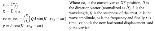
Formula used to generate the Gerstner waves
A similar effect can be generated using multiple sine waves. However, the Gerstner waves not only displace the vertices vertically, but also horizontally. In order to produce a more natural result the vertices are displaced along the X and Z axes towards the crest of the wave, resulting in a sharper peak and smoother trough, we can control the amount of displacement through the steepness parameter of the GerstnerWaveTessendorf function.
The following screenshot shows three examples of waves, the first is a regular sine wave (Gerstner wave with a steepness of 0.0), the second is the same wave except with a steepness of 0.5, and the last is a wireframe of the same wave again with a steepness of 1.0. See how the vertices in the wireframe come closer along the length of the crest.
When comparing a single wave to the gentle and choppy waves, it is fairly obvious that a good simulation of a wave requires multiple waves of varying lengths, amplitudes, directions, and possibly frequencies; these different individual wave definitions are often referred to as octaves. By summing together the entire set of waves, we achieve a more realistic and varied result. The gentle waves are generated using four octaves, while the choppy waves are generated using six octaves.
Although we have generated the waves on the GPU, it is interesting to note that if we place a ship (similar to the one in the following screenshot – section D) , we still need to compute its movement as a part of the wider physics simulation. This would most likely occur on the CPU.
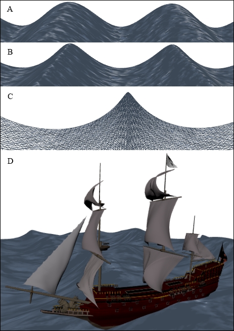
Three examples of a single wave with a length of 10 m and amplitude of 2.5 m, A) Crest steepness of 0.0, B) Crest steepness of 0.5, C) Steepness of 1.0, and D) A static ship on dynamic waves.
There are a number of methods for simulating water, depending on whether it is shallow or deep, a lake or a river, and a realistic simulation or an approximation. One such method is the combination of the Fast Fourier Transform (FFT) and Perlin Noise.
In this recipe, we looked at the wave geometry. However, for a realistic water or ocean simulation, you must consider the caustics, refraction, reflectivity, dispersion, and interactivity as well.
Providing a static value for time, adding some texture, and playing with the amplitude could also produce interesting sand dunes or other terrain such as mountains or rolling hills.
- For more information on implementing normal mapping, refer to Chapter 6, Adding Surface Detail with Normal and Displacement Mapping
- Vertex instancing and indirect draws are covered in the next recipe, Rendering particles