4. Series Impedance of Overhead and Underground Lines

Search in book...
Toggle Font Controls
Create new playlist

Name your new playlist

Playlist description (optional)
Sign In

Email address

Password

Forgot Password?

or

Continue with Facebook

Continue with Google
Sign Up

Full Name

Email address

Confirm Email Address

Password

or

Continue with Facebook

Continue with Google

The determination of the series impedance for overhead and underground lines is a critical step before the analysis of a distribution feeder can begin. The series impedance of a single-phase, two-phase (V-phase), or three-phase distribution line consists of the resistance of the conductors and the self and mutual inductive reactances resulting from the magnetic fields surrounding the conductors. The resistance component for the conductors will typically come from a table of conductor data such as that found in Appendix A.

4.1 Series Impedance of Overhead Lines

The inductive reactance (self and mutual) component of the impedance is a function of the total magnetic fields surrounding a conductor. Figure 4.1 shows conductors 1 to n with the magnetic flux lines created by currents flowing in each of the conductors.

images

Figure 4.1
Magnetic fields.

The currents in all conductors are assumed to be flowing out of the page. It is further assumed that the sum of the currents will add to zero. That is:

I 1 + I 2 + \dots + I i + \dots + I n = 0

$I_{1} + I_{2} + \dots + I_{i} + \dots + I_{n} = 0$ (4.1)

The total flux linking conductor i is given by:

λ i = 2 \cdot 10 - 7 \cdot (I 1 \cdot ln 1 D i 1 + I 2 \cdot ln 1 D i 2 + \dots + I i \cdot ln 1 GMR i + \dots + I n \cdot ln 1 D i n) W-T/m

$λ_{i} = 2 \cdot 10^{- 7} \cdot (I_{1} \cdot \ln \frac{1}{D_{i 1}} + I_{2} \cdot \ln \frac{1}{D_{i 2}} + \dots + I_{i} \cdot \ln \frac{1}{{GMR}_{i}} + \dots + I_{n} \cdot \ln \frac{1}{D_{i n}}) W-T/m$ (4.2)

where

D_in = Distance between conductor i and conductor n (ft)

GMR_i = geometric mean radius of conductor i (ft)

The inductance of conductor i consists of the “self-inductance” of conductor i and the “mutual inductance” between conductor i and all of the other n −1 conductors. By definition:

Self-inductance: L i i = λ i i I i = 2 \cdot 10 - 7 \cdot ln 1 GMR i H/m

$Self-inductance: L_{i i} = \frac{λ_{i i}}{I_{i}} = 2 \cdot 10^{- 7} \cdot \ln \frac{1}{{GMR}_{i}} H/m$ (4.3)

Mutual inductance: L i n = λ i n I n = 2 \cdot 10 - 7 \cdot ln 1 D i n H/m

$Mutual inductance: L_{i n} = \frac{λ_{i n}}{I_{n}} = 2 \cdot 10^{- 7} \cdot \ln \frac{1}{D_{i n}} H/m$ (4.4)

4.1.1 Transposed Three-Phase Lines

High-voltage transmission lines are usually assumed to be transposed (each phase occupies the same physical position on the structure for one-third of the length of the line). In addition to the assumption of transposition, it is assumed that the phases are equally loaded (balanced loading). With these two assumptions, it is possible to combine the “self” and “mutual” terms into one “phase” inductance [1].

Phase inductance: L i = 2 \cdot 10 - 7 \cdot ln D eq GMR i H/m

$Phase inductance: L_{i} = 2 \cdot 10^{- 7} \cdot \ln \frac{D_{eq}}{{GMR}_{i}} H/m$ (4.5)

where

D eq = D a b \cdot D b c \cdot D c a - - - - - - - - - - - \sqrt 3 ft

$D_{eq} = \sqrt[3]{D_{a b} \cdot D_{b c} \cdot D_{c a}} ft$ (4.6)

D_ab, D_bc, and D_ca are the distances between phases.

Assuming a frequency of 60 Hz, the phase inductive reactance is given by:

Phase reactance: x i = ω \cdot L i = 0.12134 \cdot ln D eq GMR i Ω /mile

$Phase reactance: x_{i} = ω \cdot L_{i} = 0.12134 \cdot \ln \frac{D_{eq}}{{GMR}_{i}} Ω /mile$ (4.7)

The series impedance per phase of a transposed three-phase line consisting of one conductor per phase is given by:

Series impedance: z i = r i + j \cdot 0.12134 \cdot ln D eq GMR i Ω/mile

$Series impedance: z_{i} = r_{i} + j \cdot 0.12134 \cdot \ln \frac{D_{eq}}{{GMR}_{i}} Ω/mile$ (4.8)

4.1.2 Untransposed Distribution Lines

Because distribution systems consist of single-phase, two-phase, and untransposed three-phase lines serving unbalanced loads, it is necessary to retain the identity of the self- and mutual impedance terms of the conductors in addition to taking into account the ground return path for the unbalanced currents. The resistance of the conductors is taken directly from a table of conductor data. Equations 4.3 and 4.4 are used to compute the self- and mutual inductive reactances of the conductors. The inductive reactance will be assumed to be at a frequency of 60 Hz, and the length of the conductor will be assumed to be 1 mile. With those assumptions, the self- and mutual impedances are given by:

z ¯ i i = r i + j 0.12134 \cdot ln 1 GMR i Ω/mile

${\bar{z}}_{i i} = r_{i} + j 0.12134 \cdot \ln \frac{1}{{GMR}_{i}} Ω/mile$ (4.9)

z ¯ i j = j 0.12134 \cdot ln 1 D i j Ω/mile

${\bar{z}}_{i j} = j 0.12134 \cdot \ln \frac{1}{D_{i j}} Ω/mile$ (4.10)

In 1926, John Carson published a paper in which he developed a set of equations for computing the self- and mutual impedances of lines, taking into account the return path of the current through the ground [2]. Carson’s approach was to represent a line with the conductors connected to a source at one end and grounded at the remote end. Figure 4.2 illustrates a line consisting of two conductors (i and j) carrying currents (I_i and I_j) with the remote ends of the conductors tied to the ground. A fictitious “dirt” conductor carrying current I_d is used to represent the return path for the currents.

images

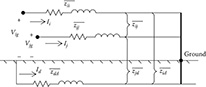
Figure 4.2
Two conductors with dirt return path.

In Figure 4.2, Kirchhoff’s voltage law (KVL) is used to write the equation for the voltage between conductor i and the ground.

V i g = z ¯ i i \cdot I i + z ¯ i j \cdot I j + z ¯ i d \cdot I d - (z ¯ d d \cdot I d + z ¯ d i \cdot I i + z ¯ d j \cdot I j)

$V_{i g} = {\bar{z}}_{i i} \cdot I_{i} + {\bar{z}}_{i j} \cdot I_{j} + {\bar{z}}_{i d} \cdot I_{d} - ({\bar{z}}_{d d} \cdot I_{d} + {\bar{z}}_{d i} \cdot I_{i} + {\bar{z}}_{d j} \cdot I_{j})$ (4.11)

Collect terms in Equation 4.11:

V i g = (z ¯ i i - z ¯ d n) \cdot I i + (z ¯ i j - z ¯ d j) \cdot I j + (z ¯ i d - z ¯ d d) \cdot I d

$V_{i g} = ({\bar{z}}_{i i} - {\bar{z}}_{d n}) \cdot I_{i} + ({\bar{z}}_{i j} - {\bar{z}}_{d j}) \cdot I_{j} + ({\bar{z}}_{i d} - {\bar{z}}_{d d}) \cdot I_{d}$ (4.12)

From Kirchhoff’s Current Law:

I i + I j + I d = 0 I d = - I i - I j

$\begin{array}{l} I_{i} + I_{j} + I_{d} = 0 \\ I_{d} = - I_{i} - I_{j} \end{array}$ (4.13)

Substitute Equation 4.13 into Equation 4.12 and collect terms:

V i g = (z ¯ i i + z ¯ d d - z ¯ d i - z ¯ i d) \cdot I i + (z ¯ i j + z ¯ d d - z ¯ d j - z ¯ i d) \cdot I j

$V_{i g} = ({\bar{z}}_{i i} + {\bar{z}}_{d d} - {\bar{z}}_{d i} - {\bar{z}}_{i d}) \cdot I_{i} + ({\bar{z}}_{i j} + {\bar{z}}_{d d} - {\bar{z}}_{d j} - {\bar{z}}_{i d}) \cdot I_{j}$ (4.14)

Equation 4.14 is of the general form:

V i g = z ˆ i i \cdot I i + z ˆ i j \cdot I j

$V_{i g} = {\hat{z}}_{i i} \cdot I_{i} + {\hat{z}}_{i j} \cdot I_{j}$ (4.15)

where

z ˆ i i = z ¯ i i + z ¯ d d - z ¯ d i - z ¯ i d

${\hat{z}}_{i i} = {\bar{z}}_{i i} + {\bar{z}}_{d d} - {\bar{z}}_{d i} - {\bar{z}}_{i d}$ (4.16)

z ˆ i j = z ¯ i j + z ¯ d d - z ¯ d j - z ¯ i d

${\hat{z}}_{i j} = {\bar{z}}_{i j} + {\bar{z}}_{d d} - {\bar{z}}_{d j} - {\bar{z}}_{i d}$ (4.17)

In Equations 4.16 and 4.17, the “hat” impedances are given by Equations 4.9 and 4.10. Note that in these two equations, the effect of the ground return path is being “folded” into what will now be referred to as the “primitive” self- and mutual impedances of the line. The “equivalent primitive circuit” is shown in Figure 4.3.

images

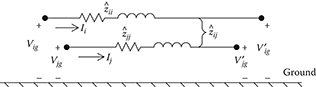
Figure 4.3
Equivalent primitive circuit.

Substituting Equations 4.9 and 4.10 of the “hat” impedances into Equations 4.16 and 4.17, the primitive self-impedance is given by:

z ˆ i i = r i + j x i i + r d + j x d d - j x d n - j x n d z ˆ i i = r d + r i + j 0.12134 \cdot (ln 1 GMR i + ln 1 GMR d - ln 1 D i d - ln 1 D d i) z ˆ i i = r d + r i + j 0.12134 \cdot (ln 1 GMR i + ln D i d \cdot D d j GMR d)

$\begin{array}{l} {\hat{z}}_{i i} = r_{i} + j x_{i i} + r_{d} + j x_{d d} - j x_{d n} - j x_{n d} \\ {\hat{z}}_{i i} = r_{d} + r_{i} + j 0.12134 \cdot (\ln \frac{1}{{GMR}_{i}} + \ln \frac{1}{{GMR}_{d}} - \ln \frac{1}{D_{i d}} - \ln \frac{1}{D_{d i}}) \\ {\hat{z}}_{i i} = r_{d} + r_{i} + j 0.12134 \cdot (\ln \frac{1}{{GMR}_{i}} + \ln \frac{D_{i d} \cdot D_{d j}}{{GMR}_{d}}) \end{array}$ (4.18)

In a similar manner, the primitive mutual impedance can be expanded:

z ˆ i j = j x i j + r d + j x d d - j x d j - j x i d z ˆ i j = r d + j 0.12134 \cdot (ln 1 D i j + ln 1 GMR d - ln 1 D d j - ln 1 D i d) z ˆ i j = r d + j 0.12134 (ln 1 D i j + ln D d j \cdot D i d GMR d)

$\begin{array}{l} {\hat{z}}_{i j} = j x_{i j} + r_{d} + j x_{d d} - j x_{d j} - j x_{i d} \\ {\hat{z}}_{i j} = r_{d} + j 0.12134 \cdot (\ln \frac{1}{D_{i j}} + \ln \frac{1}{{GMR}_{d}} - \ln \frac{1}{D_{d j}} - \ln \frac{1}{D_{i d}}) \\ {\hat{z}}_{i j} = r_{d} + j 0.12134 (\ln \frac{1}{D_{i j}} + \ln \frac{D_{d j} \cdot D_{i d}}{{GMR}_{d}}) \end{array}$ (4.19)

The obvious problem in using Equations 4.18 and 4.19 is the fact that we do not know the values of the resistance of dirt (r_d), the geometric mean radius of dirt (GMR_d), and the distances from the conductors to dirt (D_nd, D_dn, D_md, D_dm). This is where John Carson’s work bails us out.

4.1.3 Carson’s Equations

Because a distribution feeder is inherently unbalanced, the most accurate analysis should not make any assumptions regarding the spacing between conductors, conductor sizes, and transposition. In Carson’s 1926 paper, he developed a technique whereby the self- and mutual impedances for ncond overhead conductors can be determined. The equations can also be applied to underground cables. In 1926, this technique was not met with a lot of enthusiasm because of the tedious calculations that would have to be done on the slide rule and by hand. With the advent of the digital computer, Carson’s equations have now become widely used.

In his paper, Carson assumes the earth as an infinite, uniform solid, with a flat uniform upper surface and a constant resistivity. Any “end effects” introduced at the neutral grounding points are not large at power frequencies, and therefore are neglected.

Carson made use of conductor images—that is, every conductor at a given distance above ground has an image conductor at the same distance below ground. This is illustrated in Figure 4.4.

images

Figure 4.4
Conductors and images.

Referring to Figure 4.4, the original Carson equations are given in Equations 4.20 and 4.21.

Self-impedance:

z ˆ i i = r i + 4 ω P i i G + j (X i + 2 ω G \cdot ln S i i R D i + 4 ω Q i i G) Ω/mile

${\hat{z}}_{i i} = r_{i} + 4 ω P_{i i} G + j (X_{i} + 2 ω G \cdot \ln \frac{S_{i i}}{R D_{i}} + 4 ω Q_{i i} G) Ω/mile$ (4.20)

Mutual impedance:

z ˆ i j = 4 ω P i j G + j (2 ω G \cdot ln S i j D i j + 4 ω Q i j G) Ω /mile

${\hat{z}}_{i j} = 4 ω P_{i j} G + j (2 ω G \cdot \ln \frac{S_{i j}}{D_{i j}} + 4 ω Q_{i j} G) Ω /mile$ (4.21)

where

Ẑ_ii = self-impedance of conductor i in Ω/mile

Ẑ_ij = mutual impedance between conductors i and jin Ω/mile

r_i = resistance of conductor i in Ω/mile

ω = 2πf = system angular frequency in radians per second

G = 0.1609347 × 10⁻³ Ω/mile

RD_i = radius of conductor i in ft

GMR_i = geometric mean radius of conductor i in ft

f = system frequency in Hertz

ρ = resistivity of earth in Ω-meters

D_ij = distance between conductors i and j in ft (see Figure 4.4)

S_ij = distance between conductor i and image j in ft (see Figure 4.4)

θ_ij = angle between a pair of lines drawn from conductor i to its own image and to the image of conductor j (see Figure 4.4)

X i = 2 ω G \cdot ln R D i GMR i Ω/mile

$X_{i} = 2 ω G \cdot \ln \frac{R D_{i}}{{GMR}_{i}} Ω/mile$ (4.22)

P i j = π 8 - 1 3 2 - \sqrt k i j cos (θ i j) + k 2 i j 16 cos (2 θ i j) \cdot (0.6728 + ln 2 k i j)

$P_{i j} = \frac{π}{8} - \frac{1}{3 \sqrt{2}} k_{i j} \cos (θ_{i j}) + \frac{k_{i j}^{2}}{16} \cos (2 θ_{i j}) \cdot (0.6728 + \ln \frac{2}{k_{i j}})$ (4.23)

Q i j = - 0.0386 + 1 2 \cdot l n 2 k i j + 1 3 2 - \sqrt k i j c o s (θ i j)

$Q_{i j} = - 0.0386 + \frac{1}{2} \cdot l n \frac{2}{k_{i j}} + \frac{1}{3 \sqrt{2}} k_{i j} c o s (θ_{i j})$ (4.24)

k i j = 8.565 \cdot 10 - 4 \cdot S i j \cdot f ρ - - \sqrt

$k_{i j} = 8.565 \cdot 10^{- 4} \cdot S_{i j} \cdot \sqrt{\frac{f}{ρ}}$ (4.25)

4.1.4 Modified Carson’s Equations

Only two approximations are made in deriving the “Modified Carson Equations.” These approximations involve the terms associated with P_ij and Q_ij. The approximations use only the first term of the variable P_ij and the first two terms of Q_ij.

P i j = π 8

$P_{i j} = \frac{π}{8}$ (4.26)

Q i j = - 0.03860 + 1 2 ln 2 k i j

$Q_{i j} = - 0.03860 + \frac{1}{2} \ln \frac{2}{k_{i j}}$ (4.27)

Substitute X_i (Equation 4.22) into Equation 4.20:

z ˆ i i = r i + 4 ω P i i G + j (2 ϖ G \cdot ln R D i GMR i + 2 ϖ G \cdot ln S i i R D i + 4 ϖ Q i i G)

${\hat{z}}_{i i} = r_{i} + 4 ω P_{i i} G + j (2 ϖ G \cdot \ln \frac{R D_{i}}{{GMR}_{i}} + 2 ϖ G \cdot \ln \frac{S_{i i}}{R D_{i}} + 4 ϖ Q_{i i} G)$ (4.28)

Combine terms and simplify:

z ˆ i i = r i + 4 ω P i i G + j 2 ω G (ln S i i GMR i + ln R D i R D i + 2 Q i i)

${\hat{z}}_{i i} = r_{i} + 4 ω P_{i i} G + j 2 ω G (\ln \frac{S_{i i}}{{GMR}_{i}} + \ln \frac{R D_{i}}{R D_{i}} + 2 Q_{i i})$ (4.29)

Simplify Equation 4.21:

z ˆ i j = 4 ω P i j G + j 2 ω G (ln S i j D i j + 2 Q i j)

${\hat{z}}_{i j} = 4 ω P_{i j} G + j 2 ω G (\ln \frac{S_{i j}}{D_{i j}} + 2 Q_{i j})$ (4.30)

Substitute expressions for P (Equation 4.27) and ω (2 ⋅ π ⋅ f):

z ˆ i i = r i + π 2 f G + j 4 π f G (ln S i i GMR i + 2 Q i i)

${\hat{z}}_{i i} = r_{i} + π^{2} f G + j 4 π f G (\ln \frac{S_{i i}}{{GMR}_{i}} + 2 Q_{i i})$ (4.31)

z ˆ i j = π 2 f G + j 4 π f G (ln S i j D i j + 2 Q i j)

${\hat{z}}_{i j} = π^{2} f G + j 4 π f G (\ln \frac{S_{i j}}{D_{i j}} + 2 Q_{i j})$ (4.32)

Substitute expression for k_ij (Equation 4.25) into the approximate expression for Q_ij (Equation 4.27):

Q i j = - 0.03860 + 1 2 ln ⎛ ⎝ ⎜ 2 8.565 \cdot 10 - 4 \cdot S i j \cdot f ρ - - \sqrt ⎞ ⎠ ⎟

$Q_{i j} = - 0.03860 + \frac{1}{2} \ln (\frac{2}{8.565 \cdot 10^{- 4} \cdot S_{i j} \cdot \sqrt{\frac{f}{ρ}}})$ (4.33)

Expand:

Q i j = - 0.03860 + 1 2 ln (2 8.565 \cdot 10 - 4) + 1 2 ln 1 S i j + 1 2 ln ρ f - - \sqrt

$Q_{i j} = - 0.03860 + \frac{1}{2} \ln (\frac{2}{8.565 \cdot 10^{- 4}}) + \frac{1}{2} \ln \frac{1}{S_{i j}} + \frac{1}{2} \ln \sqrt{\frac{ρ}{f}}$ (4.34)

Equation 4.34 can be reduced to:

Q i j = 3.8393 - 1 2 ln S i j + 1 4 ln ρ f

$Q_{i j} = 3.8393 - \frac{1}{2} \ln S_{i j} + \frac{1}{4} \ln \frac{ρ}{f}$ (4.35)

or:

2 Q i j = 2 Q i j = 7.6786 - ln S i j + 1 2 ln ρ f

$2 Q_{i j} = 2 Q_{i j} = 7.6786 - \ln S_{i j} + \frac{1}{2} \ln \frac{ρ}{f}$ (4.36)

Substitute Equation 4.36 into Equation 4.31 and simplify:

z ˆ i i = r i + π 2 f G + j 4 π f G (ln S i i GMR i + 7.6786 - ln S i i + 1 2 ln ρ f) z ˆ i i = r i + π 2 f G + 4 π f G (ln 1 GMR i + 7.6786 + 1 2 ln ρ f)

$\begin{array}{l} {\hat{z}}_{i i} = r_{i} + π^{2} f G + j 4 π f G (\ln \frac{S_{i i}}{{GMR}_{i}} + 7.6786 - \ln S_{i i} + \frac{1}{2} \ln \frac{ρ}{f}) \\ {\hat{z}}_{i i} = r_{i} + π^{2} f G + 4 π f G (\ln \frac{1}{{GMR}_{i}} + 7.6786 + \frac{1}{2} \ln \frac{ρ}{f}) \end{array}$ (4.37)

Substitute Equation 4.36 into Equation 4.32 and simplify:

z ˆ i j = π 2 f G + j 4 π f G (ln S i j D i j + 7.6786 - ln S i j + 1 2 ln ρ f) z ˆ i j = π 2 f G + j 4 π f G (ln 1 D i j + 7.6786 + 1 2 ln ρ f)

$\begin{array}{l} {\hat{z}}_{i j} = π^{2} f G + j 4 π f G (\ln \frac{S_{i j}}{D_{i j}} + 7.6786 - \ln S_{i j} + \frac{1}{2} \ln \frac{ρ}{f}) \\ {\hat{z}}_{i j} = π^{2} f G + j 4 π f G (\ln \frac{1}{D_{i j}} + 7.6786 + \frac{1}{2} \ln \frac{ρ}{f}) \end{array}$ (4.38)

Substitute in the values of π and G:

z ˆ i i = r i + 0.00158836 \cdot f + j 0.00202237 \cdot f (ln 1 GMR i + 7.6786 + 1 2 ln ρ f)

${\hat{z}}_{i i} = r_{i} + 0.00158836 \cdot f + j 0.00202237 \cdot f (\ln \frac{1}{{GMR}_{i}} + 7.6786 + \frac{1}{2} \ln \frac{ρ}{f})$ (4.39)

z ˆ i j = 0.00158836 \cdot f + j 0.00202237 \cdot f (ln 1 D i j + 7.6786 + 1 2 ln ρ f)

${\hat{z}}_{i j} = 0.00158836 \cdot f + j 0.00202237 \cdot f (\ln \frac{1}{D_{i j}} + 7.6786 + \frac{1}{2} \ln \frac{ρ}{f})$ (4.40)

It is now assumed:

f = frequency = 60 Hertz

ρ = earth resistivity = 100 Ω-m

Using these approximations and assumptions, the “Modified Carson’s Equations” are:

z ˆ i i = r i + 0.09530 + j 0.12134 (ln 1 GMR i + 7.93402) Ω /mile

${\hat{z}}_{i i} = r_{i} + 0.09530 + j 0.12134 (\ln \frac{1}{{GMR}_{i}} + 7.93402) Ω /mile$ (4.41)

z ˆ i j = 0.09530 + j 0.12134 (ln 1 D i j + 7.93402) Ω /mile

${\hat{z}}_{i j} = 0.09530 + j 0.12134 (\ln \frac{1}{D_{i j}} + 7.93402) Ω /mile$ (4.42)

It will be recalled that Equations 4.18 and 4.19 could not be used because the resistance of dirt, the GMR_d, and the various distances from conductors to dirt were not known. A comparison of Equations 4.18 and 4.19 to Equations 4.41 and 4.42 demonstrates that the Modified Carson’s Equations have defined the missing parameters. A comparison of the two sets of equations shows that:

r d = 0.09530 Ω /mile

$r_{d} = 0.09530 Ω /mile$ (4.43)

ln D i d \cdot D d i GMR d = ln D d j \cdot D i d GMR d = 7.93402

$\ln \frac{D_{i d} \cdot D_{d i}}{{GMR}_{d}} = \ln \frac{D_{d j} \cdot D_{i d}}{{GMR}_{d}} = 7.93402$ (4.44)

The “Modified Carson’s Equations” will be used to compute the primitive self- and mutual impedances of overhead and underground lines.

4.1.5 Primitive Impedance Matrix for Overhead Lines

Equations 4.41 and 4.42 are used to compute the elements of an ncond × ncond “primitive impedance matrix.” An overhead four-wire grounded wye distribution line segment will result in a 4 × 4 matrix. For an underground-grounded wye line segment consisting of three concentric neutral cables, the resulting matrix will be 6 × 6. The primitive impedance matrix for a three-phase line consisting of m neutrals will be of the form:

[z ˆ p r i m i t i v e] = ⎡ ⎣ ⎢ ⎢ ⎢ ⎢ ⎢ ⎢ ⎢ ⎢ ⎢ ⎢ ⎢ ⎢ z ˆ a a z ˆ b a z ˆ c a - - - z ˆ n 1 a z ˆ n 2 a z ˆ n m a z ˆ a b z ˆ b b z ˆ c b - - - z ˆ n 1 b z ˆ n 2 b z ˆ n m b z ˆ a c z ˆ b c z ˆ c c - - - z ˆ n 1 c z ˆ n 2 c z ˆ n m c | | | - - - | | | z ˆ a n 1 z ˆ b n 1 z ˆ c n 1 - - - z ˆ n 1 n 1 z ˆ n 2 n 1 z ˆ n m n 1 z ˆ a n 2 z ˆ b n 2 z ˆ c n 2 - - - z ˆ n 1 n 2 z ˆ n 1 n 2 z ˆ n 2 n 2 z ˆ n 2 n 2 z ˆ n m n 2 z ˆ n m n 2 z ˆ a n m z ˆ b n m z ˆ c n m - - - z ˆ n 1 n m z ˆ n 2 n m z ˆ n m n m ⎤ ⎦ ⎥ ⎥ ⎥ ⎥ ⎥ ⎥ ⎥ ⎥ ⎥ ⎥ ⎥ ⎥

$[{\hat{z}}_{p r i m i t i v e}] = [\begin{matrix} {\hat{z}}_{a a} & {\hat{z}}_{a b} & {\hat{z}}_{a c} & | & {\hat{z}}_{a n 1} & {\hat{z}}_{a n 2} & {\hat{z}}_{a n m} \\ {\hat{z}}_{b a} & {\hat{z}}_{b b} & {\hat{z}}_{b c} & | & {\hat{z}}_{b n 1} & {\hat{z}}_{b n 2} & {\hat{z}}_{b n m} \\ {\hat{z}}_{c a} & {\hat{z}}_{c b} & {\hat{z}}_{c c} & | & {\hat{z}}_{c n 1} & {\hat{z}}_{c n 2} & {\hat{z}}_{c n m} \\ - - - & - - - & - - - & - - - & - - - & - - - & - - - \\ {\hat{z}}_{n 1 a} & {\hat{z}}_{n 1 b} & {\hat{z}}_{n 1 c} & | & {\hat{z}}_{n 1 n 1} & {\hat{z}}_{n 1 n 2} {\hat{z}}_{n 1 n 2} & {\hat{z}}_{n 1 n m} \\ {\hat{z}}_{n 2 a} & {\hat{z}}_{n 2 b} & {\hat{z}}_{n 2 c} & | & {\hat{z}}_{n 2 n 1} & {\hat{z}}_{n 2 n 2} {\hat{z}}_{n 2 n 2} & {\hat{z}}_{n 2 n m} \\ {\hat{z}}_{n m a} & {\hat{z}}_{n m b} & {\hat{z}}_{n m c} & | & {\hat{z}}_{n m n 1} & {\hat{z}}_{n m n 2} {\hat{z}}_{n m n 2} & {\hat{z}}_{n m n m} \end{matrix}]$ (4.45)

In partitioned form, Equation 4.45 becomes:

[z ˆ p r i m i t i v e] = [[z ˆ i j] [z ˆ n j] [z ˆ i n] [z ˆ n n]]

$[{\hat{z}}_{p r i m i t i v e}] = [\begin{matrix} [{\hat{z}}_{i j}] & [{\hat{z}}_{i n}] \\ [{\hat{z}}_{n j}] & [{\hat{z}}_{n n}] \end{matrix}]$ (4.46)

4.1.6 Phase Impedance Matrix for Overhead Lines

For most applications, the primitive impedance matrix needs to be reduced to a 3 × 3 “phase frame” matrix consisting of the self- and mutual equivalent impedances for the three phases. A four-wire grounded neutral line segment is shown in Figure 4.5.

images

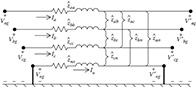
Figure 4.5
Four-wire grounded wye line segment.

One standard method of reduction is the “Kron” reduction [3]. It is assumed that the line has a multigrounded neutral (Figure 4.5). The Kron reduction method applies KVL to the circuit.

$[\begin{matrix} V_{a g} \\ V_{b g} \\ V_{c g} \\ V_{n g} \end{matrix}] = [\begin{matrix} {V^{'}}_{a g} \\ {V^{'}}_{b g} \\ {V^{'}}_{c g} \\ {V^{'}}_{n g} \end{matrix}] + [\begin{matrix} {\hat{z}}_{a a} & {\hat{z}}_{a b} & {\hat{z}}_{a c} & {\hat{z}}_{a n} \\ {\hat{z}}_{b a} & {\hat{z}}_{b b} & {\hat{z}}_{b c} & {\hat{z}}_{b n} \\ {\hat{z}}_{c a} & {\hat{z}}_{c b} & {\hat{z}}_{c c} & {\hat{z}}_{c n} \\ {\hat{z}}_{n a} & {\hat{z}}_{n b} & {\hat{z}}_{n c} & {\hat{z}}_{n n} \end{matrix}] \cdot [\begin{matrix} I_{a} \\ I_{b} \\ I_{c} \\ I_{n} \end{matrix}]$ (4.47)

In partitioned form, Equation 4.47 becomes:

$[\begin{matrix} [V_{a b c}] \\ [V_{n g}] \end{matrix}] = [\begin{matrix} [{V^{'}}_{a b c}] \\ [{V^{'}}_{n g}] \end{matrix}] + [\begin{matrix} [{\hat{z}}_{i j}] & [{\hat{z}}_{i n}] \\ [{\hat{z}}_{n g}] & [{\hat{z}}_{n n}] \end{matrix}] \cdot [\begin{matrix} [I_{a b c}] \\ [I_{n}] \end{matrix}]$ (4.48)

Because the neutral is grounded, the voltages V_ng and V′_ng are equal to zero. Substituting those values into Equation 4.48 and expanding results in:

$[V_{a b c}] = [{V^{'}}_{a b c}] + [{\hat{z}}_{i j}] \cdot [I_{a b c}] + [{\hat{z}}_{i n}] \cdot [I_{n}]$ (4.49)

$[0] = [0] + [{\hat{z}}_{n j}] \cdot [I_{a b c}] + [{\hat{z}}_{n n}] \cdot [I_{n}]$ (4.50)

Solve Equation 4.50 for [I_n]:

$[I_{n}] = - {[{\hat{z}}_{n n}]}^{- 1} \cdot [{\hat{z}}_{n j}] \cdot [I_{a b c}]$ (4.51)

Note in Equation 4.51 that once the line currents have been computed, it is possible to determine the current flowing in the neutral conductor. Because this will be a useful concept later on, the “neutral transformation matrix” is defined as:

$[t_{n}] = - {[{\hat{z}}_{n n}]}^{- 1} \cdot [{\hat{z}}_{n j}]$ (4.52)

Such that:

$[I_{n}] = [t_{n}] \cdot [I_{a b c}]$ (4.53)

Substitute Equation 4.51 into Equation 4.49:

$[V_{a b c}] = [{V^{'}}_{a b c}] + ([{\hat{z}}_{i j}] - [{\hat{z}}_{i n}] \cdot {[{\hat{z}}_{n n}]}^{- 1} \cdot [{\hat{z}}_{n j}]) \cdot [I_{a b c}] [V_{a b c}] = [{V^{'}}_{a b c}] + [z_{a b c}] \cdot [I_{a b c}]$ (4.54)

where

$[z_{a b c}] = [{\hat{z}}_{i j}] - [{\hat{z}}_{i n}] \cdot {[{\hat{z}}_{n n}]}^{- 1} \cdot [{\hat{z}}_{n j}]$ (4.55)

Equation 4.55 is the final form of the “Kron” reduction technique. The final phase impedance matrix becomes:

$[z_{a b c}] = [\begin{matrix} z_{a a} & z_{a b} & z_{a c} \\ z_{b a} & z_{b b} & z_{b c} \\ z_{c a} & z_{c b} & z_{c c} \end{matrix}] Ω /mile$ (4.56)

For a distribution line that is not transposed, the diagonal terms of Equation 4.56 will not be equal to each other and the off-diagonal terms will not be equal to each other. However, the matrix will be symmetrical.

For two-phase (V-phase) and single-phase lines in grounded wye systems, the Modified Carson’s Equations can be applied, which will lead to initial 3 × 3 and 2 × 2 primitive impedance matrices. Kron reduction will reduce the matrices to 2 × 2 and a single element. These matrices can be expanded to 3 × 3 “phase frame” matrices by the addition of rows and columns consisting of zero elements for the missing phases. For example, for a V-phase line consisting of phases a and c, the phase impedance matrix would be:

$[z_{a b c}] = [\begin{matrix} z_{a a} & 0 & z_{a c} \\ 0 & 0 & 0 \\ z_{c a} & 0 & z_{c c} \end{matrix}] Ω /mile$ (4.57)

The phase impedance matrix for a phase b single-phase line would be:

$[z_{a b c}] = [\begin{matrix} 0 & 0 & 0 \\ 0 & z_{b b} & 0 \\ 0 & 0 & 0 \end{matrix}] Ω /mile$ (4.58)

The phase impedance matrix for a three-wire delta line is determined by the application of Carson’s equations without the Kron reduction step.

The phase impedance matrix can be used to accurately determine the voltage drops on the feeder line segments once the currents have been determined. Because no approximations (transposition, for example) have been made regarding the spacing between conductors, the effect of the mutual coupling between phases is accurately taken into account. The application of the Modified Carson’s Equations and the phase frame matrix leads to the most accurate model of a line segment. Figure 4.6 shows the general three-phase model of a line segment. Keep in mind that for V-phase and single-phase lines, some of the impedance values will be zero.

images

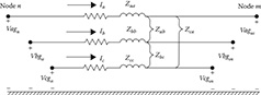
Figure 4.6
Three-phase line segment model.

The voltage equation in matrix form for the line segment is:

${[\begin{matrix} V_{a g} \\ V_{b g} \\ V_{c g} \end{matrix}]}_{n} = {[\begin{matrix} V_{a g} \\ V_{b g} \\ V_{c g} \end{matrix}]}_{m} + [\begin{matrix} Z_{a a} & Z_{a b} & Z_{a c} \\ Z_{b a} & Z_{b b} & Z_{b c} \\ Z_{c a} & Z_{c b} & Z_{c c} \end{matrix}] \cdot [\begin{matrix} I_{a} \\ I_{b} \\ I_{c} \end{matrix}]$ (4.59)

where $Z_{i j} = z_{i j} \cdot length$ .

Equation 4.59 can be written in “condensed” form as:

${[V_{L G}_{_{a b c}}]}_{n} = {[V_{L G}_{_{a b c}}]}_{m} + [Z_{a b c}] \cdot [I_{a b c}]$ (4.60)

4.1.7 Sequence Impedances

Mostly, the analysis of a feeder will use only the positive and zero sequence impedances for the line segments. There are two methods for obtaining these impedances. The first method incorporates the application of the Modified Carson’s Equations and the Kron reduction to obtain the phase impedance matrix.

The definition for line-to-ground phase voltages as a function of the line-to-ground sequence voltages is given by Carson [2]:

$[\begin{matrix} V_{a g} \\ V_{b g} \\ V_{c g} \end{matrix}] = [\begin{matrix} 1 & 1 & 1 \\ 1 & a_{s}^{2} & a_{s} \\ 1 & a_{s} & a_{s}^{2} \end{matrix}] \cdot [\begin{matrix} V_{0 g} \\ V_{1 g} \\ V_{2 g} \end{matrix}]$ (4.61)

where $a_{s} = 1.0 / 120_$ .

In condensed form, Equation 4.61 becomes:

$[V_{L G}_{_{a b c}}] = [A_{s}] \cdot [V_{L G}_{_{012}}]$ (4.62)

where

$[A_{s}] = [\begin{matrix} 1 & 1 & 1 \\ 1 & a_{s}^{2} & a_{s} \\ 1 & a_{s} & a_{s}^{2} \end{matrix}]$ (4.63)

The phase line currents are defined in the same manner:

$[I_{a b c}] = [A_{s}] \cdot [I_{012}]$ (4.64)

Equation 4.62 can be used to solve for the sequence line-to-ground voltages as a function of the phase line-to-ground voltages.

$[V_{L G}_{_{012}}] = {[A_{s}]}^{- 1} \cdot [V_{L G}_{_{a b c}}]$ (4.65)

where

${[A_{s}]}^{- 1} = \frac{1}{3} \cdot [\begin{matrix} 1 & 1 & 1 \\ 1 & a_{s} & a_{s}^{2} \\ 1 & a_{s}^{2} & a_{s} \end{matrix}]$ (4.66)

Equation 4.60 can be transformed to the sequence domain by multiplying both sides by [A_s]⁻¹ and also substituting in the definition of the phase currents as given by Equation 4.62.

$\begin{array}{l} {[V_{L G}_{_{012}}]}_{n} = {[A_{s}]}^{- 1} \cdot {[V_{L G}_{_{a b c}}]}_{n} \\ {[V_{L G}_{_{012}}]}_{n} = {[A_{s}]}^{- 1} \cdot {[V_{L G}_{_{a b n}}]}_{m} + {[A_{s}]}^{- 1} \cdot [Z_{a b c}] \cdot [A_{s}] \cdot [I_{012}] \\ {[V_{L G}_{_{012}}]}_{n} = {[V_{L G}_{_{012}}]}_{m} + [Z_{012}] \cdot [I_{012}] \end{array}$ (4.67)

where

$[Z_{012}] = {[A_{s}]}^{- 1} \cdot [Z_{a b c}] \cdot [A_{s}] = [\begin{matrix} Z_{00} & Z_{01} & Z_{02} \\ Z_{10} & Z_{11} & Z_{12} \\ Z_{20} & Z_{21} & Z_{22} \end{matrix}]$ (4.68)

Equation 4.67 in expanded form is given by:

${[\begin{matrix} V_{0 g} \\ V_{1 g} \\ V_{2 g} \end{matrix}]}_{n} = {[\begin{matrix} V_{0 g} \\ V_{1 g} \\ V_{2 g} \end{matrix}]}_{m} + [\begin{matrix} Z_{00} & Z_{01} & Z_{02} \\ Z_{10} & Z_{11} & Z_{02} \\ Z_{20} & Z_{21} & Z_{22} \end{matrix}] \cdot [\begin{matrix} I_{0} \\ I_{1} \\ I_{2} \end{matrix}]$ (4.69)

Equation 4.68 is the defining equation for converting phase impedances to sequence impedances. In Equation 4.68, the diagonal terms of the matrix are the “sequence impedances” of the line such that:

Z₀₀ = zero sequence impedance

Z₁₁ = positive sequence impedance

Z₂₂ = negative sequence impedance

The off-diagonal terms of Equation 4.68 represent the mutual coupling between sequences. In the idealized state, these off-diagonal terms would be zero. In order for this to happen, it must be assumed that the line has been transposed. For high-voltage transmission lines, this will generally be the case. When the lines are transposed, the mutual coupling between phases (off-diagonal terms) are equal, and consequently the off-diagonal terms of the sequence impedance matrix become zero. Because distribution lines are rarely if ever transposed, the mutual coupling between phases is not equal, and as a result, the off-diagonal terms of the sequence impedance matrix will not be zero. This is the primary reason that distribution system analysis uses the phase domain rather than symmetrical components.

If a line is assumed to be transposed, the phase impedance matrix is modified so that the three diagonal terms are equal and all of the off-diagonal terms are equal. A different method to compute the sequence impedances is to set the three diagonal terms of the phase impedance matrix equal to the average of the diagonal terms of Equation 4.56 and the off-diagonal terms equal to the average of the off-diagonal terms of Equation 4.56. When this is done, the self- and mutual impedances are defined as:

$z_{s} = \frac{1}{3} \cdot (z_{a a} + z_{b b} + z_{c c}) Ω / m i l e$ (4.70)

$z_{m} = \frac{1}{3} (z_{a b} + z_{b c} + z_{c a}) Ω / m i l e$ (4.71)

The phase impedance matrix is now defined as:

$[z_{a b c}] = [\begin{matrix} z_{s} & z_{m} & z_{m} \\ z_{m} & z_{s} & z_{m} \\ z_{m} & z_{m} & z_{s} \end{matrix}] Ω / m i l e$ (4.72)

When Equation 4.68 is used with this phase impedance matrix, the resulting sequence matrix is diagonal (off-diagonal terms are zero). The sequence impedances can be determined directly as:

$z_{00} = z_{s} + 2 \cdot z_{m} Ω / m i l e$ (4.73)

$z_{11} = z_{22} = z_{s} - z_{m} Ω / mile$ (4.74)

A second method that is commonly used to determine the sequence impedances directly is to employ the concept of geometric mean distances (GMDs). The GMD between phases is defined as:

$D_{i j} = G M D_{i j} = \sqrt[3]{D_{a b} \cdot D_{b c} \cdot D_{c a}} f t$ (4.75)

The GMD between phases and neutral is defined as:

$D_{i n} = G M D_{i n} = \sqrt[3]{D_{a n} \cdot D_{b n} \cdot D_{c n}} f t$ (4.76)

The GMDs as defined previously are used in Equations 4.41 and 4.42 to determine the various self- and mutual impedances of the line resulting in:

${\hat{z}}_{i i} = r_{i} + 0.0953 + j 0.12134 \cdot [l n (\frac{1}{G M R_{i}}) + 7.93402] Ω / m i l e$ (4.77)

${\hat{z}}_{n n} = r_{n} + 0.0953 + j 0.12134 \cdot [l n (\frac{1}{G M R_{n}}) + 7.93402] Ω / m i l e$ (4.78)

${\hat{z}}_{i j} = 0.0953 + j 0.12134 \cdot [l n (\frac{1}{D_{i j}}) + 7.93402] Ω / m i l e$ (4.79)

${\hat{z}}_{i n} = 0.0953 + j 0.12134 \cdot [l n (\frac{1}{D_{i n}}) + 7.93402] Ω / m i l e$ (4.80)

Equations 4.77 through 4.80 will define a matrix of order ncond × ncond where ncond is the number of conductors (phases plus neutrals) in the line segment. Application of the Kron reduction (Equation 4.55) and the sequence impedance transformation (Equation 4.68) leads to the following expressions for the zero, positive, and negative sequence impedances:

$z_{00} = {\hat{z}}_{i i} + 2 \cdot {\hat{z}}_{i j} - 3 \cdot (\frac{{\hat{z}}_{i n}^{2}}{{\hat{z}}_{n n}}) Ω / m i l e$ (4.81)

$\begin{array}{l} z_{11} = z_{22} = {\hat{z}}_{i i} - {\hat{z}}_{i j} \\ z_{11} = z_{22} = r_{i} + j 0.12134 \cdot l n (\frac{D_{i j}}{G M R_{i}}) Ω / m i l e \end{array}$ (4.82)

Equations 4.81 and 4.82 are recognized as the standard equations for the calculation of the line impedances when a balanced three-phase system and transposition are assumed.

Example 4.1

An overhead three-phase distribution line is constructed as shown in Figure 4.7. Determine the phase impedance matrix and the positive and zero sequence impedance matrices of the line. The phase conductors are 336,400 26/7 ACSR (Linnet), and the neutral conductor is 4/0 6/1 ACSR.

images

Figure 4.7
Three-phase distribution line spacings.

Solution: From the table of standard conductor data (Appendix A), it is found that:

336,400 26/7 ACSR: GMR = 0.0244 ft

Resistance = 0.306 Ω/mile

4/0 6/1 ACSR: GMR = 0.00814 ft

Resistance = 0.5920 Ω/mile

An effective way of computing the distance between all conductors is to specify each position on the pole in Cartesian coordinates using complex number notation. The ordinate will be selected as a point on the ground directly below the leftmost position. For the line in Figure 4.7, the positions are:

$d_{1} = 0 + j 29 d_{2} = 2.5 + j 29 d_{3} = 7.0 + j 29 d_{4} = 4.0 + j 25$

The distances between the positions can be computed as:

$D_{12} = | d_{1} - d_{2} | D_{23} = | d_{2} - d_{3} | D_{31} = | d_{3} - d_{1} |$

$D_{14} = | d_{1} - d_{4} | D_{24} = | d_{2} - d_{4} | D_{34} = | d_{3} - d_{4} |$

For this example, phase a is in position 1, phase b is in position 2, phase c is in position 3, and the neutral is in position 4.

$D_{a b} = 2 . 5^{'} D_{b c} = 4 . 5^{'} D_{c a} = 7 . 0^{'}$

$D_{a n} = 5.656 9^{'} D_{b n} = 4.27 2^{'} D_{c n} = 5 . 0^{'}$

The diagonal terms of the distance matrix are the GMRs of the phase and neutral conductors.

$D_{a a} = D_{b b} = D_{c c} = 0.0244 D_{n n} = 0.00814$

Applying the Modified Carson’s Equation for self-impedance (Equation 4.41), the self-impedance for phase a is:

${\hat{z}}_{a a} = 0.0953 + 0.306 + j 0.12134 \cdot (\ln \frac{1}{0.0244} + 7.93402) = 0.4013 + j 1.4133 Ω / m i l e$

Applying Equation 4.42 for the mutual impedance between phases a and b:

${\hat{z}}_{a b} = 0.0953 + j 0.12134 \cdot (\ln \frac{1}{2.5} + 7.93402) = 0.0953 + j 0.8515 Ω / m i l e$

Applying the equations for the other self- and mutual impedance terms results in the primitive impedance matrix.

$[\hat{z}] = [\begin{matrix} 0.4013 + j 1.4133 & 0.0953 + j 0.8515 & 0.0953 + j 0.7266 & 0.0953 + j 0.7524 \\ 0.0953 + j 0.8515 & 0.4013 + j 1.4133 & 0.0953 + j 0.7802 & 0.0953 + j 0.7865 \\ 0.0953 + j 0.7266 & 0.0953 + j 0.7802 & 0.4013 + j 1.4133 & 0.0953 + j 0.7674 \\ 0.0953 + j 0.7524 & 0.0953 + j 0.7865 & 0.0953 + j 0.7674 & 0.6873 + j 1.5465 \end{matrix}] Ω / m i l e$

The primitive impedance matrix in partitioned form is:

$[{\hat{z}}_{i j}] = [\begin{matrix} 0.4013 + j 1.4133 & 0.0953 + j 0.8515 & 0.0953 + j 0.7266 \\ 0.0953 + j 0.8515 & 0.4013 + j 1.4133 & j 0.0943 + j 0.7865 \\ 0.0953 + j 0.7266 & 0.0953 + j 0.7802 & 0.4013 + j 1.4133 \end{matrix}] Ω / m i l e$

$[{\hat{z}}_{i n}] = [\begin{matrix} 0.0953 + j 0.7524 \\ 0.0953 + j 0.7865 \\ 0.0953 + j 0.7674 \end{matrix}] Ω / m i l e$

$[{\hat{z}}_{n n}] = [0.6873 + j 1.5465] Ω / m i l e$

$[{\hat{z}}_{n j}] = [\begin{matrix} 0.0953 + j 0.7524 & 0.0953 + j 0.7865 & 0.0953 + j 0.7674 \end{matrix}] Ω / m i l e$

The “Kron” reduction of Equation 4.55 results in the “phase impedance matrix.”

$[z_{a b c}] = [{\hat{z}}_{i j}] - [{\hat{z}}_{i n}] \cdot {[{\hat{z}}_{n n}]}^{- 1} \cdot [{\hat{z}}_{n j}]$

$[z_{a b c}] = [\begin{matrix} 0.4576 + j 1.0780 & 0.1560 + j .5017 & 0.1535 + j 0.3849 \\ 0.1560 + j 0.5017 & 0.4666 + j 1.0482 & 0.1580 + j 0.4236 \\ 0.1535 + j 0.3849 & 0.1580 + j 0.4236 & 0.4615 + j 1.0651 \end{matrix}] Ω / m i l e$

The neutral transformation matrix given by Equation 4.52 is:

$\begin{array}{l} [t_{n}] = - ({[{\hat{z}}_{n n}]}^{- 1} \cdot [{\hat{z}}_{n j}]) \\ [t_{n}] = [\begin{matrix} - 0.4292 - j 0.1291 & - 0.4476 - j 0.1373 & - 0.4373 - j 0.1327 \end{matrix}] \end{array}$

The phase impedance matrix can be transformed into the “sequence impedance matrix” with the application of Equation 4.66.

$[z_{012}] = {[A_{s}]}^{- 1} \cdot [z_{a b c}] \cdot [A_{s}]$

$[z_{012}] = [\begin{matrix} 0.7735 + j 1.9373 & 0.0256 + j 0.0115 & - 0.0321 + j 0.0159 \\ - 0.0321 + j 0.0159 & 0.3061 + j 0.6270 & - 0.0723 - j 0.0060 \\ 0.0256 + j 0.0115 & 0.0723 - j 0.0059 & 0.3061 + j 0.6270 \end{matrix}] Ω / m i l e$

In the sequence impedance matrix, the 1,1 term is the zero sequence impedance, the 2,2 term is the positive sequence impedance, and the 3,3 term is the negative sequence impedance. The 2,2 and 3,3 terms are equal, which demonstrates that for line segments, the positive and negative sequence impedances are equal. Note that the off-diagonal terms are not zero. This implies that there is mutual coupling between sequences. This is a result of the nonsymmetrical spacing between phases. With the off-diagonal terms being nonzero, the three sequence networks representing the line will not be independent. However, it is noted that the off-diagonal terms are small relative to the diagonal terms.

In high-voltage transmission lines, it is usually assumed that the lines are transposed and that the phase currents represent a balanced three-phase set. The transposition can be simulated in Example 4.1 by replacing the diagonal terms of the phase impedance matrix with the average value of the diagonal terms (0.4619 + j1.0638) and replacing each off-diagonal term with the average of the off-diagonal terms (0.1558 + j0.4368). This modified phase impedance matrix becomes:

$[z_{1}_{_{a b c}}] = [\begin{matrix} 0.4619 + j 1.0638 & 0.1558 + j 0.4368 & 0.1558 + j 0.4368 \\ 0.1558 + j 0.4368 & 0.4619 + j 1.0638 & 0.1558 + j 0.4368 \\ 0.1558 + j 0.4368 & 0.1558 + j 0.4368 & 0.4619 + j 1.0638 \end{matrix}] Ω / m i l e$

Using this modified phase impedance matrix in the symmetrical component transformation equation results in the modified sequence impedance matrix.

$[z_{1}_{_{012}}] = [\begin{matrix} 0.7735 + j 1.9373 & 0 & 0 \\ 0 & 0.3061 + j 0.6270 & 0 \\ 0 & 0 & 0.3061 + j 0.6270 \end{matrix}] Ω / m i l e$

Note now that the off-diagonal terms are all equal to zero, which means that there is no mutual coupling between sequence networks. It should also be noted that the modified zero, positive, and negative sequence impedances are exactly equal to the exact sequence impedances that were first computed.

The results of this example should not be interpreted to mean that a three-phase distribution line could be assumed to have been transposed. The original phase impedance matrix should be used if the correct effect of the mutual coupling between phases is to be modeled.

4.1.8 Parallel Overhead Distribution Lines

It is fairly common in a distribution system to find instances where two distribution lines are “physically” parallel. The parallel combination may have both distribution lines constructed on the same pole, or the two lines may run in parallel on separate poles but on the same right-of-way. For example, two different feeders leaving a substation may share a common pole or right-of-way before they branch out to their own service area. It is also possible that two feeders may converge and run in parallel until again they branch out into their own service areas. The lines could also be underground circuits sharing a common trench. In all of the cases, the question arises as to how the parallel lines should be modeled and analyzed.

Two parallel overhead lines on one pole are shown in Figure 4.8.

images

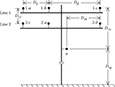
Figure 4.8
Parallel overhead lines.

Note in Figure 4.8 the phasing of the two lines.

The phase impedance matrix for the parallel distribution lines is computed by the application of Carson’s equations and the Kron reduction method. The first step is to number the phase positions as follows:

images

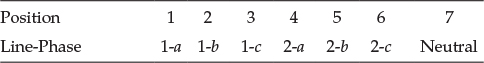
With the phases numbered, the 7 × 7 primitive impedance matrix for 1 mile can be computed using the Modified Carson’s Equations. It should be pointed out that if the two parallel lines are on different poles, most likely each pole will have a grounded neutral conductor. In this case, there will be 8 positions, and position 8 will correspond to the neutral on line 2. An 8 × 8 primitive impedance matrix will be developed for this case. The Kron reduction will reduce the matrix to a 6 × 6 phase impedance matrix. With reference to Figure 4.8, the voltage drops in the two lines are given by:

$[\begin{matrix} v_{1}_{_{a}} \\ v_{1}_{_{b}} \\ v_{1}_{_{c}} \\ v_{2}_{_{a}} \\ v_{2}_{_{b}} \\ v_{2}_{_{c}} \end{matrix}] = [\begin{matrix} z_{11}_{_{a a}} & z_{11}_{_{a b}} & z_{11}_{_{a c}} & z_{12}_{_{a a}} & z_{12}_{_{a b}} & z_{12}_{_{a c}} \\ z_{11}_{_{b a}} & z_{11}_{_{b b}} & z_{11}_{_{b c}} & z_{12}_{_{b a}} & z_{12}_{_{b b}} & z_{12}_{_{b c}} \\ z_{11}_{_{c a}} & z_{11}_{_{c b}} & z_{11}_{_{c c}} & z_{12}_{_{c a}} & z_{12}_{_{c b}} & z_{12}_{_{c c}} \\ z_{21_{a a}} & z_{21}_{_{a b}} & z_{21}_{_{a c}} & z_{22}_{_{a a}} & z_{22}_{_{a b}} & z_{22}_{_{a c}} \\ z_{21}_{_{b a}} & z_{21}_{_{b b}} & z_{21}_{_{b c}} & z_{22}_{_{b a}} & z_{22}_{_{b b}} & z_{22}_{_{b c}} \\ z_{21}_{_{c a}} & z_{21}_{_{c b}} & z_{21}_{_{c c}} & z_{22}_{_{c a}} & z_{22}_{_{c b}} & z_{22}_{_{c c}} \end{matrix}] \cdot [\begin{matrix} I_{1}_{_{a}} \\ I_{1}_{_{b}} \\ I_{1}_{_{c}} \\ I_{2}_{_{a}} \\ I_{2}_{_{b}} \\ I_{2}_{_{c}} \end{matrix}]$ (4.83)

Partition Equation 4.83 between the third and fourth rows and columns, so that series voltage drops for 1 mile of line are given by:

$[v] = [z] \cdot [I] = [\begin{matrix} [v_{1}] \\ [v_{2}] \end{matrix}] = [\begin{matrix} [z_{11}] & [z_{12}] \\ [z_{21}] & [z_{22}] \end{matrix}] \cdot [\begin{matrix} [I_{1}] \\ [I_{2}] \end{matrix}] V$ (4.84)

Example 4.2

Two parallel distribution lines are on a single pole (Figure 4.9).

images

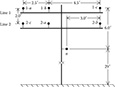
Figure 4.9
Example parallel OH lines.

The phase conductors are:

Line 1: 336,400 26/7 ACSR: GMR₁ = 0.0244′ r₁ =0.306 Ω/mile d₁ = 0.721″

Line 2: 250,000 AA: GMR₂ = 0.0171′ r₂ = 0.41 Ω/mile d₂ = 0.567″

Neutral: 4/06/1 ACSR: GMR_n = 0.00814′ r_n = 0.592 Ω/mile d_n = 0.563″

Determine the 6 × 6 phase impedance matrix.

Define the conductor positions according to the phasing:

$\begin{array}{l} d_{1} = 0 + j 35 d_{2} = 2.5 + j 35 d_{3} = 7 + j 35 \\ d_{4} = 2.5 + j 33 d_{5} = 7 + j 33 d_{6} = 0 + j 33 \\ d_{7} = 4 + j 29 \end{array}$

Using $D_{i j} = | d_{i} - d_{j} |$ , the distances between all conductors can be computed. Using this equation, the diagonal terms of the resulting spacing matrix will be zero. It is convenient to define the diagonal terms of the spacing matrix as the GMR of the conductors occupying the position. Using this approach, the final spacing matrix is:

$[D] = [\begin{matrix} 0.0244 & 2.5 & 7 & 3.2016 & 7.2801 & 2 & 7.2111 \\ 2.5 & 0.0244 & 4.5 & 2 & 4.9244 & 3.2016 & 6.1847 \\ 7 & 4.5 & 0.0244 & 4.9244 & 2 & 7.2801 & 6.7082 \\ 3.2016 & 2 & 4.9244 & 0.0171 & 4.5 & 2.5 & 4.2720 \\ 7.2801 & 4.9244 & 2 & 4.5 & 0.0171 & 7 & 5 \\ 2 & 3.2016 & 7.2801 & 2.5 & 7 & 0.0171 & 5.6869 \\ 7.2111 & 6.1847 & 6.7082 & 4.2720 & 5 & 5.6569 & 0.0081 \end{matrix}]$

The terms for the primitive impedance matrix can be computed using the Modified Carson’s Equations. For this example, the subscripts i and j will run from 1 to 7. The 7 × 7 primitive impedance matrix is partitioned between rows and columns 6 and 7. The Kron reduction will now give the final phase impedance matrix. In partitioned form, the phase impedance matrices are:

${[z_{11}]}_{a b c} = [\begin{matrix} 0.4502 + j 1.1028 & 0.1464 + j 0.5334 & 0.1452 + j 0.4126 \\ 0.1464 + j 0.5334 & 0.4548 + j 1.0873 & 0.1475 + j 0.4584 \\ 0.1452 + j 0.4126 & 0.1475 + j 0.4584 & 0.4523 + j 1.0956 \end{matrix}] Ω / m i l e$

${[z_{12}]}_{a b c} = [\begin{matrix} 0.1519 + j 0.4848 & 0.1496 + j 0.3931 & 0.1477 + j 0.5560 \\ 0.1545 + j 0.5336 & 0.1520 + j 0.4323 & 0.1502 + j 0.4909 \\ 0.1531 + j 0.4287 & 0.1507 + j 0.5460 & 0.1489 + j 0.3955 \end{matrix}] Ω / m i l e$

${[z_{21}]}_{a b c} = [\begin{matrix} 0.1519 + j 0.4848 & 0.1545 + j 0.5336 & 0.1531 + j 0.4287 \\ 0.1496 + j 0.3931 & 0.1520 + j 0.4323 & 0.1507 + j 0.5460 \\ 0.1477 + j 0.5560 & 0.1502 + j 0.4909 & 0.1489 + j 0.3955 \end{matrix}] Ω / m i l e$

${[z_{22}]}_{a b c} = [\begin{matrix} 0.5706 + j 1.0913 & 0.1580 + j 0.4236 & 0.1559 + j 0.5017 \\ 0.1580 + j 0.4236 & 0.5655 + j 1.1082 & 0.1535 + j 0.3849 \\ 0.1559 + j 0.5017 & 0.1535 + j 0.3849 & 0.5616 + j 1.1212 \end{matrix}] Ω / m i l e$

4.2 Series Impedance of Underground Lines

Figure 4.10 shows the general configuration of three underground cables (concentric neutral or tape-shielded) with an additional neutral conductor.

images

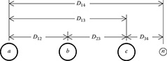
Figure 4.10
Three-phase underground with additional neutral.

The Modified Carson’s Equations can be applied to underground cables in much the same manner as for overhead lines. The circuit in Figure 4.10 will result in a 7 × 7 primitive impedance matrix. For underground circuits that do not have the additional neutral conductor, the primitive impedance matrix will be 6 × 6.

Two popular types of underground cables are the “concentric neutral cable” and the “tape shield cable.” To apply the Modified Carson’s Equations, the resistance and GMR of the phase conductor and the equivalent neutral must be known.

4.2.1 Concentric Neutral Cable

Figure 4.11 shows a simple detail of a concentric neutral cable. The cable consists of a central “phase conductor” covered by a thin layer of nonmetallic semiconducting screen to which is bonded the insulating material. The insulation is then covered by a semiconducting insulation screen. The solid strands of concentric neutral are spiraled around the semiconducting screen with a uniform spacing between strands. Some cables will also have an insulating “jacket” encircling the neutral strands.

images

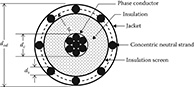
Figure 4.11
Concentric neutral cable.

In order to apply Carson’s equations to this cable, the following data needs to be extracted from a table of underground cables (Appendices A and B).

d_c = phase conductor diameter (in.)

d_od = nominal diameter over the concentric neutrals of the cable (in.)

d_s = diameter of a concentric neutral strand (in.)

GMR_c = geometric mean radius of the phase conductor (ft)

GMR_s = geometric mean radius of a neutral strand (ft)

r_c = resistance of the phase conductor (Ω/mile)

r_s = resistance of a solid neutral strand (Ω/mile)

k = number of concentric neutral strands

The GMRs of the phase conductor and a neutral strand are obtained from a standard table of conductor data (Appendix A). The equivalent GMR of the concentric neutral is computed using the equation for the GMR of bundled conductors used in high-voltage transmission lines [2].

${GMR}_{c n} = \sqrt[k]{{GMR}_{s} \cdot k \cdot R^{k - 1}} f t$ (4.85)

where

R = radius of a circle passing through the center of the concentric neutral strands

$R = \frac{d_{od} - d_{s}}{24} ft$ (4.86)

The equivalent resistance of the concentric neutral is:

$r_{c n} = \frac{r_{s}}{k} Ω /mile$ (4.87)

The various spacings between a concentric neutral and the phase conductors and other concentric neutrals are as follows:

Concentric Neutral to Its Own Phase Conductor

D_ij = R (Equation 4.86)

Concentric Neutral to an Adjacent Concentric Neutral

D_ij = center-to-center distance of the phase conductors

Concentric Neutral to an Adjacent Phase Conductor

Figure 4.12 shows the relationship between the distance between centers of concentric neutral cables and the radius of a circle passing through the centers of the neutral strands.

images

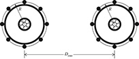
Figure 4.12
Distances between concentric neutral cables.

The GMD between a concentric neutral and an adjacent phase conductor is given by:

$D_{i j} = \sqrt[k]{D_{n m}^{k} - R^{k}} ft$ (4.88)

where D_nm = center-to-center distance between phase conductors.

The distance between cables will be much greater than the radius R; so a good approximation of modeling the concentric neutral cables is shown in Figure 4.13. In this figure, the concentric neutrals are modeled as one equivalent conductor (shown in black) directly above the phase conductor.

images

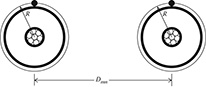
Figure 4.13
Equivalent neutral cables.

In applying the Modified Carson’s Equations, the numbering of conductors and neutrals is important. For example, a three-phase underground circuit with an additional neutral conductor must be numbered as:

1 = phase a Conductor #1

2 = phase b Conductor #2

3 = phase c Conductor #3

4 = neutral of Conductor #1

5 = neutral of Conductor #2

6 = neutral of Conductor #3

7 = additional neutral conductor (if present)

Example 4.3

Three concentric neutral cables are buried in a trench with spacings as shown in Figure 4.14.

images

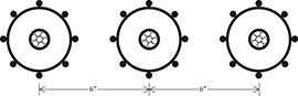
Figure 4.14
Three-phase concentric neutral cable spacing.

The concentric neutral cables of Figure 4.14 can be modeled as shown in Figure 4.15. Notice the numbering of the phase conductors and the equivalent neutrals.

images

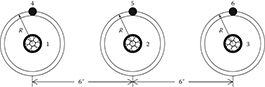
Figure 4.15
Three-phase equivalent concentric neutral cable spacing.

The cables are 15 kV, 250,000 CM stranded all aluminum with k = 13 strands of #14 annealed coated copper wires (1/3 neutral). The outside diameter of the cable over the neutral strands is 1.29 in. (Appendix B). Determine the phase impedance matrix and the sequence impedance matrix.

Solution: The data for the phase conductor and neutral strands from a conductor data table (Appendix A) are:

250,000 AA phase conductor:

GMR_p = 0.0171 ft

Diameter = 0.567 in.

Resistance = 0.4100 Ω/mile#

#14 copper neutral strands:

GMR_s = 0.00208 ft

Resistance = 14.87 Ω/mile

Diameter (d_s) = 0.0641 in.

The radius of the circle passing through the center of the strands (Equation 4.82) is:

$R = \frac{d_{od} - d_{s}}{24} = 0.0511 ft$

The equivalent GMR of the concentric neutral is computed by:

${GMR}_{c n} = \sqrt[k]{{GMR}_{s} \cdot k \cdot R^{k - 1}} = \sqrt[13]{0.00208 \cdot 13 \cdot {0.0511}^{13 - 1}} = 0.0486 ft$

The equivalent resistance of the concentric neutral is:

$r_{c n} = \frac{r_{s}}{k} = \frac{14.8722}{13} = 1.1438 Ω /mile$

The phase conductors are numbered 1, 2, and 3. The concentric neutrals are numbered 4, 5, and 6.

A convenient method of computing the various spacings is to define each conductor using Cartesian coordinates. Using this approach, the conductor coordinates are:

$\begin{array}{l} d_{1} = 0 + j 0 d_{2} = 0.5 + j 0 d_{3} = 1 + 1 j 0 \\ d_{4} = 0 + j R d_{5} = 0.5 + j R d_{6} = 1 + j R \end{array}$

The spacings of off-diagonal terms of the spacing matrix are computed by:

$\begin{array}{l} For: n = 1 to 6 and m = 1 to 6 \\ D_{n, m} = | d_{n} - d_{m} | \end{array}$

The diagonal terms of the spacing matrix are the GMRs of the phase conductors and the equivalent neutral conductors:

$\begin{array}{l} For i = 1 to 3 and j = 4 to 6 \\ D_{i, i} = {GMR}_{p} \\ D_{j, j} = {GMR}_{s} \end{array}$

The resulting spacing matrix is:

$[D] = [\begin{matrix} 0.0171 & 0.5 & 1 & 0.0511 & 0.5026 & 1.0013 \\ 0.5 & 0.0171 & 0.5 & 0.5026 & 0.0511 & 0.5026 \\ 1 & 0.5 & 0.0171 & 1.0013 & 0.5026 & 0.0511 \\ 0.0511 & 0.5026 & 1.0013 & 0.0486 & 0.5 & 1 \\ 0.5026 & 0.0511 & 0.5026 & 0.5 & 0.0486 & 0.5 \\ 1.0013 & 0.5026 & 0.0511 & 1 & 0.5 & 0.0486 \end{matrix}] ft.$

The self-impedance for the cable in position 1 is:

${\hat{z}}_{11} = 0.0953 + 0.41 + j 0.12134 \cdot (\ln \frac{1}{0.0171} + 7.93402) = 0.5053 + j 1.4564 Ω /mile$

The self-impedance for the concentric neutral for Cable #1 is:

${\hat{z}}_{44} = 0.0953 + 1.144 + j 0.12134 \cdot (\ln \frac{1}{0.0486} + 7.93402) = 1.2391 + j 1.3296 Ω /mile$

The mutual impedance between Cable #1 and Cable #2 is:

${\hat{z}}_{12} = 0.0953 + j 0.12134 \cdot (\ln \frac{1}{0.5} + 7.93402) = 0.0953 + j 1.0468 Ω /mile$

The mutual impedance between Cable #1 and its concentric neutral is:

${\hat{z}}_{14} = 0.0953 + j 0.12134 \cdot (\ln \frac{1}{0.0511} + 7.93402) = 0.0953 + j 1.3236 Ω /mile$

The mutual impedance between the concentric neutral of Cable #1 and the concentric neutral of Cable #2 is:

${\hat{z}}_{45} = 0.0953 + j 0.12134 \cdot (\ln \frac{1}{0.5} + 7.93402) = 0.0953 + j 1.0468 Ω /mile$

Continuing the application of the Modified Carson’s Equations results in a 6 × 6 primitive impedance matrix. This matrix in partitioned (Equation 4.33) form is:

$[{\hat{z}}_{i j}] = [\begin{matrix} 0.5053 + j 1.4564 & 0.0953 + j 1.0468 & 0.0953 + j .9627 \\ 0.0953 + j 1.0468 & 0.5053 + j 1.4564 & 0.0953 + j 1.0468 \\ 0.0953 + j .9627 & 0.0953 + j 1.0468 & 0.5053 + j 1.4564 \end{matrix}] Ω /mile$

$[{\hat{z}}_{i n}] = [\begin{matrix} 0.0953 + j 1.3236 & 0.0953 + j 1.0468 & 0.0953 + j .9627 \\ 0.0953 + j 1.0462 & 0.0953 + j 1.3236 & 0.0953 + j 1.0462 \\ 0.0953 + j .9626 & 0.0953 + j 1.0462 & 0.0953 + j 1.3236 \end{matrix}] Ω /mile$

$[{\hat{z}}_{n j}] = [{\hat{z}}_{i n}]$

$[{\hat{z}}_{n n}] = [\begin{matrix} 1.2393 + j 1.3296 & 0.0953 + j 1.0468 & 0.0953 + j .9627 \\ 0.0953 + j 1.0468 & 1.2393 + j 1.3296 & 0.0953 + j 1.0468 \\ 0.0953 + j .9627 & 0.0953 + j 1.0468 & 1.2393 + j 1.3296 \end{matrix}] Ω /mile$

Using the Kron reduction results in the phase impedance matrix:

$[z_{a b c}] = [{\hat{z}}_{i j}] - [{\hat{z}}_{i n}] \cdot {[{\hat{z}}_{n n}]}^{- 1} \cdot [{\hat{z}}_{n j}]$

$[z_{a b c}] = [\begin{matrix} 0.7981 + j 0.4467 & 0.3188 + j 0.0334 & 0.2848 - j 0.0138 \\ 0.3188 + j 0.0334 & 0.7890 + j 0.4048 & 0.3188 + j 0.0334 \\ 0.2848 - j 0.0138 & 0.3188 + j 0.0334 & 0.7981 + j 0.4467 \end{matrix}] Ω /mile$

The sequence impedance matrix for the concentric neutral three-phase line is determined using Equation 4.68.

$[z_{012}] = {[A_{s}]}^{- 1} \cdot [z_{a b c}] \cdot [A_{s}]$

$[z_{012}] = [\begin{matrix} 1.4140 + j 0.4681 & - 0.0026 - j 0.0081 & - 0.0057 + j 0.0063 \\ - 0.0057 + j 0.0063 & 0.4876 + j 0.4151 & - 0.0265 + j 0.0450 \\ - 0.0026 - j 0.0081 & 0.0523 + j 0.0004 & 0.4876 + j 0.4151 \end{matrix}] Ω /mile$

4.2.2 Tape-Shielded Cables

Figure 4.16 shows a simple detail of a tape-shielded cable. The cable consists of a central “phase conductor” covered by a thin layer of nonmetallic semiconducting screen to which is bonded the insulating material. The insulation is covered by a semiconducting insulation screen. The shield is bare copper tape helically applied around the insulation screen. An insulating “jacket” encircles the tape shield.

images

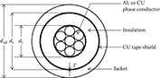
Figure 4.16
Tape-shielded cable.

Parameters of the tape-shielded cable are:

d_c = diameter of phase conductor (in.): Appendix A

d_s = outside diameter of the tape shield (in.): Appendix B

d_od = outside diameter over jacket (in.): Appendix B

T = thickness of copper tape shield in mils: Appendix B

Once again, the Modified Carson’s Equations will be applied to calculate the self-impedances of the phase conductor and the tape shield as well as the mutual impedance between the phase conductor and the tape shield. The resistance and GMR of the phase conductor are found in a standard table of conductor data (Appendix A).

The resistance of the tape shield is given by:

$r_{shield} = 1.0636 \cdot 10^{9} \cdot \frac{ρ m_{20}}{d_{s} \cdot T} Ω /mile$ (4.89)

The resistance of the tape shield given in Equation 4.89 assumes a resistivity (ρm₂₀) of 1.7721 · 10⁻⁸ Ω-m and a temperature of 20°C. The outside diameter of the tape shield d_s is given in inches, and the thickness of the tape shield T is in mils.

The GMR of the tape shield is the radius of a circle passing through the middle of the shield and is given by:

${GMR}_{shield} = \frac{\frac{d_{s}}{2} - \frac{T}{2000}}{12} ft$ (4.90)

The various spacings between a tape shield and the conductors and other tape shields are as follows:

Tape Shield to its Own Phase Conductor

$D_{i j} = {GMR}_{shield} = radius to midpoint of the shield (ft)$ (4.91)

Tape Shield to an Adjacent Tape Shield

$D_{i j} = Center-to-center distance of the phase conductors(ft)$ (4.92)

Tape Shield to an Adjacent Phase or Neutral Conductor

$D_{i j} = D_{n m} ft$ (4.93)

where D_nm = center-to-center distance between phase conductors.

Example 4.4

A single-phase circuit consists of a 1/0 AA, 220 mil insulation tape-shielded cable and a 1/0 CU neutral conductor (Figure 4.17). The single-phase line is connected to phase b. Determine the phase impedance matrix.

images

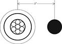
Figure 4.17
Single-phase tape shield with neutral conductor.

Cable data: 1/0 AA

Outside diameter of the tape shield = d_s = 0.88 in.

Resistance = 0.97 Ω/mile

GMR_p = 0.0111 ft

Tape shield thickness = T = 5 mils

Resistivity = ρm₂₀ = 1.7721 ⋅ 10⁻⁸ Ω-m

Neutral data: 1/0 Copper, 7 strand

Resistance = 0.607 Ω/mile

GMR_n = 0.01113 ft

Distance between cable and neutral = D_nm = 3 in.

The resistance of the tape shield is computed according to Equation 4.89:

$r_{shield} = \frac{1.0636 \cdot 10^{9} \cdot ρ m_{20}}{d_{s} \cdot T} = \frac{18.8481}{0.88 \cdot 5} = 4.2836 Ω /mile$

The GMR of the tape shield is computed according to Equation 4.90:

${GMR}_{shield} = \frac{\frac{d_{s}}{2} - \frac{T}{2000}}{12} = \frac{\frac{0.88}{2} - \frac{5}{2000}}{12} = 0.0365 ft$

The conductors are numbered such that:

#1 = 1/0 AA conductor

#2 = tape shield

#3 = 1/0 copper ground

The spacings used in the Modified Carson’s Equations are:

$\begin{array}{l} D_{12} = {GMR}_{shield} = 0.0365 \\ D_{13} = \frac{3}{12} = 0.25 \end{array}$

The self-impedance of Conductor #1 is:

${\hat{z}}_{11} = 0.0953 + 0.97 + j 0.12134 \cdot (\ln \frac{1}{0.0111} + 7.93402) = 1.0653 + j 1.5088 Ω /mile$

The mutual impedance between Conductor #1 and the tape shield (Conductor #2) is:

${\hat{z}}_{12} = 0.0953 + j 0.12134 \cdot (\ln \frac{1}{0.0365} + 7.93402) = 0.0953 + j 1.3645 Ω /mile$

The self-impedance of the tape shield (Conductor #2) is:

${\hat{z}}_{22} = 0.0953 + 4.2786 + j 0.12134 \cdot (\ln \frac{1}{0.0365} + 7.93402) = 4.3739 + j 1.3645 Ω /mile$

Continuing on the final primitive impedance matrix is:

$[\hat{z}] = [\begin{matrix} 1.0653 + j 1.5088 & 0.0953 + j 1.3645 & 0.0953 + 1.1309 \\ 0.0953 + j 1.3645 & 4.3739 + j 1.3645 & 0.0953 + j 1.1309 \\ 0.0953 + j 1.1309 & 0.0953 + j 1.1309 & 0.7023 + j 1.5085 \end{matrix}] Ω /mile$

In partitioned form, the primitive impedance matrix is:

$\begin{array}{l} [{\hat{z}}_{i j}] = 1.0653 + j 1.5088 \\ [{\hat{z}}_{i n}] = [\begin{matrix} 0.0953 + j 1.3645 & 0.0953 + j 1.1309 \end{matrix}] \\ [{\hat{z}}_{n j}] = [\begin{matrix} 0.0953 + j 1.3645 \\ 0.0953 + j 1.1309 \end{matrix}] \\ [{\hat{z}}_{n n}] = [\begin{matrix} 4.3739 + j 1.3645 & 0.0953 + j 1.1309 \\ 0.0953 + j 1.1309 & 0.7023 + j 1.5085 \end{matrix}] Ω /mile \end{array}$

Applying Kron’s reduction method will result in a single impedance, which represents the equivalent single-phase impedance of the tape shield cable and the neutral conductor.

$z_{1 p} = [{\hat{z}}_{i j}] - [{\hat{z}}_{i n}] \cdot {[{\hat{z}}_{n n}]}^{- 1} \cdot [{\hat{z}}_{n j}]$

$z_{1 p} = 1.3218 + j 0.6744 Ω /mile$

Because the single-phase line is on phase b, the phase impedance matrix for the line is:

$[z_{a b c}] = [\begin{matrix} 0 & 0 & 0 \\ 0 & 1.3218 + j 0.6744 & 0 \\ 0 & 0 & 0 \end{matrix}] Ω /mile$

4.2.3 Parallel Underground Distribution Lines

The procedure for computing the phase impedance matrix for two overhead parallel lines has been presented in Section 4.1.8. Figure 4.18 shows two concentric neutral parallel lines each with a separate grounded neutral conductor.

images

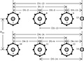
Figure 4.18
Parallel concentric neutral underground lines.

The process for computing the 6 × 6 phase impedance matrix follows exactly the same procedure as for the overhead lines. In this case, there are a total of 14 conductors (6 phase conductors, 6 equivalent concentric neutral conductors, and 2 grounded neutral conductors). Applying Carson’s equations will result in a 14 × 14 primitive impedance matrix. This matrix is partitioned between the sixth and seventh rows and columns. The Kron reduction is applied to form the final 6 × 6 phase impedance matrix.

Example 4.5

Two concentric neutral three-phase underground parallel lines are shown in Figure 4.19.

images

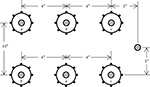
Figure 4.19
Parallel concentric neutral three-phase lines.

Cables (both lines): 250 kcmil, 1/3 neutral

Extra neutral: 4/0 Copper

Determine the 6 × 6 phase impedance matrix.

Solution: From Appendix B for the cables:

Outside diameter: d_od = 1.29″

Neutral strands: k = 13 #14 copper strands

From Appendix A for the conductors:

$250 kcmil Al : {GMR}_{c} = 0.017 1^{'}, r_{c} = 0.41 Ω /mile, d_{c} = 0.56 7^{″}$

$# 14 Copper: {GMR}_{s} = 0.0020 8^{'}, r_{s} = 14.8722 Ω /mile, d_{s} = 0.064 1^{″}$

$4 / 0 Copper : {GMR}_{n} = 0.1579', r_{n} = 0.303 Ω /mile, d_{n} = 0.522 "$

The radius of the circle to the center of the strands is:

$R_{b} = \frac{d_{od} - d_{s}}{24} = \frac{1.29 - 0.0641}{24} = 0.0511'$

The equivalent GMR of the concentric neutral strands is computed as:

${GMR}_{eq} = \sqrt[k]{{GMR}_{s} \cdot k \cdot R_{b}^{k - 1}} = \sqrt[13]{0.00208 \cdot 13 \cdot {0.05111}^{12}} = 0.0486'$

The positions of the six cables and extra neutral using Cartesian coordinates with the phase a cable in line 1 (top line) as the ordinate are shown below. Note the phasing in both lines.

$Phase a, line 1 : d_{1} = 0 + j 0 Phase b, line 1 : d_{2} = \frac{4}{12} + j 0 Phase c, line 1 : d_{3} = \frac{8}{12} + j 0$

$Phase a, line 2 : d_{4} = \frac{4}{12} - j \frac{10}{12} Phase b, line 2 : d_{5} = 0 - j \frac{10}{12} Phase c, line 2 : d_{6} = \frac{8}{12} - j \frac{10}{12}$

Equivalent neutrals:

$Phase a, line 1 : d_{7} = d_{1} + j R_{b} Phase b, line 1 : d_{8} = d_{2} + j R_{b} Phase c, line 1 : d_{9} = d_{3} + j R_{b}$

$Phase a, line 2 : d_{10} = d_{4} + j R_{b} Phase b, line 2 : d_{11} = d_{5} + j R_{b} Phase c, line 2 : d_{12} = d_{6} + j R_{b}$

Extra neutral:

$d_{13} = \frac{10}{12} - j \frac{5}{12}$

The spacing matrix defining the distances between conductors can be computed by:

$\begin{array}{l} i = 1 to 13 j = 1 to 13 \\ D_{i, j} = | d_{i} - d_{j} | \end{array}$

The diagonal terms of the spacing matrix are defined as the appropriate GMR:

$D_{1, 1} = D_{2, 2} = D_{3, 3} = D_{4, 4} = D_{5, 5} = D_{6, 6} = {GMR}_{c} = 0.0171'$

$D_{7, 7} = D_{8, 8} = D_{9, 9} = D_{10, 10} = D_{11, 11} = D_{12, 12} = {GMR}_{eq} = 0.0486'$

$D_{13, 13} = {GMR}_{n} = 0.01579'$

The resistance matrix is defined as:

$r_{1} = r_{2} = r_{3} = r_{4} = r_{5} = r_{6} = 0.41 Ω /mile$

$r_{7} = r_{8} = r_{9} = r_{10} = r_{11} = r_{12} = \frac{r_{s}}{k} = \frac{14.8722}{13} = 1.144 Ω /mile$

$r_{13} = r_{n} = 0.303 Ω /mile$

The primitive impedance matrix (13 × 13) is computed using Carson’s equations:

$\begin{array}{l} i = 1 to 13 j = 1 to 13 \\ z p_{i, j} = 0.0953 + j 0.12134 \cdot (\ln (\frac{1}{D_{i, i}}) + 7.93402) \\ z p_{i, i} = r_{i} + 0.0953 + j 0.12134 \cdot (\ln (\frac{1}{D_{i, j}}) + 7.93402) \end{array}$

Once the primitive impedance matrix is developed, it is partitioned between the sixth and seventh rows and columns, and the Kron reduction method is applied to develop the 6 × 6 phase impedance matrix. The phase impedance matrix in partitioned form is:

${[z_{11}]}_{a b c} = [\begin{matrix} 0.6450 + j 0.4327 & 0.1805 + j 0.0658 & 0.1384 + j 0.0034 \\ 0.1805 + j 0.0658 & 0.6275 + j 0.3974 & 0.1636 + j 0.0552 \\ 0.1384 + j 0.0034 & 0.1636 + j 0.0552 & 0.6131 + j 0.4081 \end{matrix}] Ω /mile$

${[z_{12}]}_{a b c} = [\begin{matrix} 0.1261 - j 0.0086 & 0.1389 + j 0.071 & 0.0782 - j 0.0274 \\ 0.1185 - j 0.0165 & 0.1237 - j 0.0145 & 0.0720 - j 0.0325 \\ 0.1083 - j 0.0194 & 0.1074 - j 0.0246 & 0.0725 - j 0.0257 \end{matrix}] Ω /mile$

${[z_{21}]}_{a b c} = [\begin{matrix} 0.1261 - j 0.0086 & 0.1185 - j 0.0165 & 0.1083 - j 0.0195 \\ 0.1389 + j 0.0071 & 0.1237 - j 0.0145 & 0.1074 - j 0.0246 \\ 0.0782 - j 0.0274 & 0.072 - j 0.0325 & 0.0725 - j 0.0257 \end{matrix}] Ω /mile$

${[z_{22}]}_{a b c} = [\begin{matrix} 0.6324 + j 0.4329 & 0.1873 + j 0.0915 & 0.0776 - j 0.0233 \\ 0.1873 + j 0.0915 & 0.6509 + j 0.4508 & 0.0818 - j 0.0221 \\ 0.0776 - j 0.0233 & 0.0818 - j 0.0221 & 0.8331 + j 0.6476 \end{matrix}] Ω /mile$

4.3 Summary

This chapter has been devoted to presenting methods for computing the phase impedances and sequence impedances of overhead lines and underground cables. Carson’s equations have been modified to simplify the computation of the phase impedances. When using the Modified Carson’s Equations, there is no need to make any assumptions, such as transposition of the lines. By assuming an untransposed line and including the actual phasing of the line, the most accurate values of the phase impedances, self and mutual, are determined. It is highly recommended that no assumptions be made in the computation of the impedances. Because voltage drop is a primary concern on a distribution line, the impedances used for the line must be as accurate as possible. This chapter also included the process of applying Carson’s equations to two distribution lines that are physically parallel. This same approach would be taken when there are more than two lines physically parallel.

Problems

4.1 The configuration and conductors of a three-phase overhead line is shown in Figure 4.20.

images

Figure 4.20
Three-phase configuration for Problem 4.1.

Phase conductors:556,500 26/7 ACSR

Neutral conductor:4/0 ACSR

1 Determine the phase impedance matrix [Z_abc] in Ω/mile.

2 Determine the sequence impedance matrix [Z₀₁₂] in Ω/mile.

3 Determine the neutral transformation matrix [t_n].

4.2 Determine the phase impedance [Z_abc] matrix in Ω/mile for the two-phase configuration in Figure 4.21.

images

Figure 4.21
Two-phase configuration for Problem 4.2.

Phase conductors: 336,400 26/7 ACSR

Neutral conductor: 4/0 6/1 ACSR

4.3 Determine the phase impedance [Z_abc] matrix in Ω/mile for the single-phase configuration shown in Figure 4.22.

images

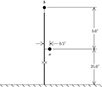
Figure 4.22
Single-phase pole configuration for Problem 4.3.

Phase and Neutral Conductors: 1/0 6/1 ACSR

4.4 Create the spacings and configurations of Problems 4.1, 4.2, and 4.3 in the distribution analysis program WindMil. Compare the phase impedance matrices to those computed in the previous problems.

4.5 Determine the phase impedance matrix [Z_abc] and sequence impedance matrix [Z₀₁₂] in Ω/mile for the three-phase pole configuration in Figure 4.23. The phase and neutral conductors are 250,000 all aluminum.

Figure 4.23
Three-phase pole configuration for Problem 4.5.

4.6 Compute the positive, negative, and zero sequence impedances in Ω/1000 ft using the GMD method for the pole configuration shown in Figure 4.23.

4.7 Determine the [Z_abc] and [Z₀₁₂ matrices in Ω/mile for the three-phase configuration shown in Figure 4.24. The phase conductors are 350,000 all aluminum, and the neutral conductor is 250,000 all aluminum.

Figure 4.24
Three-phase pole configuration for Problem 4.7.

4.8 Compute the positive, negative, and zero sequence impedances in Ω/1000 ft for the line of Figure 4.24 using the average self- and mutual impedances defined in Equations 4.70 and 4.71.

4.9 A 4/0 aluminum concentric neutral cable is to be used for a single-phase lateral. The cable has a full neutral (see Appendix B). Determine the impedance of the cable and the resulting phase impedance matrix in Ω/mile, assuming the cable is connected to phase b.

4.10 Three 250,000 CM aluminum concentric cables with one-third neutrals are buried in a trench in a horizontal configuration (see Figure 4.14). Determine the [Z_abc] and [Z₀₁₂] matrices in Ω/1000 ft assuming phasing of c–a–b.

4.11 Create the spacings and configurations of Problems 4.9 and 4.10 in WindMil. Compare the values of the phase impedance matrices to those computed in the previous problems. In order to check the phase impedance matrix, it will be necessary for you to connect the line to a balanced three-phase source. A source of 12.47 kV works fine.

4.12 A single-phase underground line is composed of a 350,000 CM aluminum tape-shielded cable. A 4/0 copper conductor is used as the neutral. The cable and neutral are separated by 4 in. Determine the phase impedance matrix in Ω/mile for this single-phase cable line assuming phase c.

4.13 Three one-third neutral 2/0 aluminum jacketed concentric neutral cables are installed in a 6-in. conduit. Assume the cable jacket has a thickness of 0.2 in. and the cables lie in a triangular configuration inside the conduit. Compute the phase impedance matrix in Ω/mile for this cabled line.

4.14 Create the spacing and configuration of Problem 4.13 in WindMil. Connect a 12.47 kV source to the line, and compare results to those of 4.13.

4.15 Two three-phase distribution lines are physically parallel as shown in Figure 4.25.

images

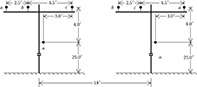
Figure 4.25
Parallel OH lines.

Line # 1 (left side): Phase conductors = 266,800 26/7 ACSR

Neutral conductor = 3/0 6/1 ACSR

Line # 2 (right side): Phase conductors = 300,000 CON LAY Aluminum

Neutral conductor = 4/0 CLASS A Aluminum

a. Determine the 6 × 6 phase impedance matrix.

b. Determine the neutral transform matrix.

4.16 Two concentric neutral underground three-phase lines are physically parallel as shown in Figure 4.26.

images

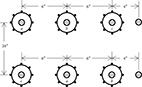
Figure 4.26
Parallel concentric neutral three-phase lines for Problem 4.16.

Line # 1 (top): Cable = 250 kcmil, 1/3 neutral

Additional neutral: 4/0 6/1 ACSR

Line #2 (bottom): Cable = 2/0 kcmil, 1/3 neutral

Additional neutral: 2/0 ACSR

a. Determine the 6 × 6 phase impedance matrix.

b. Determine the neutral transform matrix.

WindMil Assignment

Follow the method outlined in the User’s Manual to build a system called “System 1” in WindMil that will have the following components:

• 12.47 kV line-to-line source. The “Bus Voltage” should be set to 120 V

• Connect to the node and call it Node 1

• A 10,000 ft long overhead three-distribution line as defined in Problem 4.1. Call this line OH-1.

• Connect a node to the end of the line and call it Node 2.

• A wye-connected unbalanced three-phase load is connected to Node 2 and is modeled as constant PQ load with values of:

• Phase a–g: 1000 kVA, Power factor = 90% lagging

• Phase b–g: 800 kVA, Power factor = 85% lagging

• Phase c–g: 1200 kVA, Power factor = 95% lagging

Determine the voltages on a 120 V base at Node 2 and the current flowing on the OH-1 line.

References

1. Glover, J. D. and Sarma, M., Power System Analysis and Design, 2nd Edition, PWS-Kent Publishing, Boston, MA, 1994.

2. Carson, J. R., Wave propagation in overhead wires with ground return, Bell System Technical Journal, Vol. 5, pp. 539–554, 1926.

3. Kron, G., Tensorial analysis of integrated transmission systems, part I, the six basic reference frames, Transactions of the American Institute of Electrical Engineers, Vol. 71, pp. 814–882, 1952.

..................Content has been hidden....................

You can't read the all page of ebook, please click here login for view all page.

Table of Contents for
4. Series Impedance of Overhead and Underground Lines