In this chapter, you will:
Explore new and improved data features in Excel
Learn how to get help easily when working with formulas
Work with structured table references in formulas
Understand how to resolve errors in formulas
Discover how to streamline your Excel workbooks
Get sorting and filtering essentials
For those of you who hesitate to delve into the world of Microsoft Excel because you don’t like math, I’d like to start this chapter with a little story.
I dropped precalculus twice during high school. Yes, I used to be a ranking member of the math-phobic society. Ironically, by some odd stroke of luck, I placed out on the math achievement test in my senior year. So, I wasn’t required to take math in college. It was a dream come true until the start of graduate business school, where linear calculus was required for my first economics class. I was terrified. Thankfully, my economics professor did something I never thought anyone could do—the wonderful Dr. G. helped me understand the relevance of the math needed for his class. I then found, much to my astonishment, that I actually enjoy math.
This newfound appreciation for the beauty of mathematical logic enabled me a few years later to embrace Microsoft Excel, and I learned something I like even more. That is, Excel is actually the ideal program for anyone suffering from a math phobia, because Excel does the math for you.
With this story in mind, I want to welcome all math lovers and math phobics alike to this chapter on working with data in Excel. Though I hope you’ll discover more useful math-related tools than you knew before, as well as find tips and best practices for getting more from the number-crunching powers of Excel, very little knowledge of math or affection for the subject is actually required here.
The most important advance for the features and concepts addressed in this chapter is simply new and improved tools for the way you work with and present your data. Though that might sound too basic to spark your interest, it’s rather terrific in this case. From newly added sparklines, which let you chart your data in a single cell, to enhanced sorting and filtering features, such as instant search for your filters, the beauty of the Excel functionality addressed in this chapter is that doing just about anything you need to do with data can be truly and undeniably easy. A few of the marvelously simple timesavers for each version are outlined in the lists that follow.
Note
See Also For more information on sparklines, see Chapter 19.
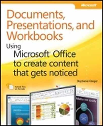
Excel 2007 added table headers that replace regular worksheet headers at the top of columns when you scroll down in a long table. Excel 2010 takes this feature one step further and keeps your filter and sort options at the top of the columns too, as shown in Figure 18-1, removing the need to freeze your panes just to access these valuable tools.
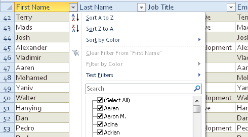
If you’re a data analyst, the Solver add-in, shown in Figure 18-2, has been redesigned for Excel 2010. Along with new solving methods, other enhancements include the ability to step through trial solutions and reuse your constraint models. To check out the enhanced Solver:
Click the File tab, click Options, and then click Add-Ins.
At the bottom of the dialog box, from the Manage drop-down, select Excel Add-Ins, and then click Go.
Select Solver Add-In, and then click OK.
After the Solver add-in is loaded, on the Data tab, in the Analysis group, click Solver.
For the number crunchers who work with millions of rows of data and think Excel is too limiting, well, it isn’t anymore. The exclusive PowerPivot for Excel 2010 is a free data analysis add-in that helps you overcome the existing limitations of working with large amounts of data on your desktop. It also integrates with SharePoint 2010 so you can turn your workbooks into shared applications and share them with others in the cloud.
Note
See Also For more on sorting and filtering, see the section2 Simplifying Data Organization, later in this chapter. For more information on PowerPivot and PowerPivot for SharePoint, and to download the add-in, go to www.powerpivot.com.
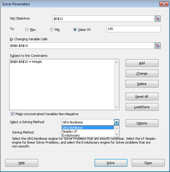
One of the key changes in Excel for Mac 2011 is the way you access functions and data tools. The Formulas tab, shown in Figure 18-3, organizes formula tools that were previously spread across several menus and gives you easier access to them.
The embedded Formula bar has finally arrived. That means each of your workbooks now has its own independent Formula bar, shown in Figure 18-4, which appears right above the worksheet column headings. And, because the Formula bar now belongs to the workbook window instead of the application (this is an Excel 2011 exclusive, by the way), you can easily compare formulas between workbooks.
The greatly improved tables feature (the evolution of Excel lists) includes powerful built-in data management capabilities, such as creating structured table references that use table element names in a formula, as shown in Figure 18-5.
Note
See Also For help creating and formatting Excel tables, see Chapter 17.
As previously mentioned, sorting and filtering capabilities are much improved. Along with new sort options, such as sorting and filtering by color and new built-in quick filters, now you can select multiple items to filter without using a custom or advanced filter, as shown in Figure 18-6. Filtering and sorting is covered in more detail later in this chapter.
The default 1904 date system is no more. Excel 2011 now uses the 1900 date system by default, which gives new workbooks date system compatibility between Mac and Windows automatically. And, exclusively in Excel 2011, you no longer need to carefully check your dates when you copy and paste them between workbooks—Excel 2011 will recognize if you’re using two date systems and prompt you accordingly, as shown in Figure 18-7.
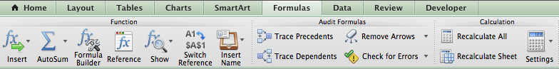
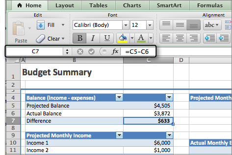
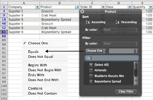
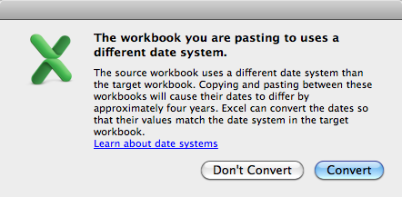
Figure 18-7. Excel 2011 will prompt you when using two different date systems instead of automatically shifting the dates by four years and one day.
Note
See Also For information explaining the two date systems, see the Microsoft Knowledge Base article 180162, available at http://support.microsoft.com/kb/180162. Note that this article was written prior to the current release of Office for Mac, so it still refers to behavior of Excel for Mac in previous versions.
When you format a range in Excel as a table, you get a working set of data instead of a simple worksheet of values. Once you’ve created that table, take advantage of the following data management capabilities.
Note
See Also To learn how to format a range as a table, see Chapter 17.
When you need a column of formulas for your data range, such as sums or averages for each row, you’ll save time if you add those formulas after your range has been formatted as a table. Tables provide a feature called Calculated Columns that enables you to add a column of formulas to the table just by adding a formula into any cell of an empty table column. When you do, the entire column populates with the same formula. In fact, if you then change that formula in any cell of the calculated column, all other cells in that column automatically update to match.
To add a calculated column to the right of existing table columns, just create a single formula in any cell of the column adjacent to the right edge of the table. The table will automatically expand and create the calculated column at the same time. Additionally, when you expand the table to add rows, the calculated column will continue to fill new cells with the same formula.
When you add a total row to a table, the functions you place in that row are interchangeable. To do this, on the Table Tools Design contextual tab (Tables tab in Excel 2011) in the Table Options group, click Total Row to add a total row to the bottom of the table. In Excel 2010, you can also right-click in the table, point to Table, and then click Totals Row.
The total row appears with a formula in the total row cell for the last column. If the data in the last column is numeric, a sum of visible cells appears in the last cell in the total row. Otherwise, a count of visible cells appears in that cell.
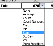
You can drag the fill handle (the box at the bottom-right corner of a selected cell) to the left to fill the same formula into other cells in that row, if appropriate. However, each cell in the total row has an available drop-down list of function options, as you see in Figure 18-8.
Note that when you choose one of the eight shortcut options available from this drop-down list, the function is actually inserted as an option of the SUBTOTAL function that performs your selected calculation type on only visible cells.
Additionally, if you add a formula in the row directly beneath a table that doesn’t have a total row, one will automatically be added. However, if it doesn’t already use a SUBTOTAL option, the formula you entered won’t be changed to one of the SUBTOTAL function options automatically. To use a SUBTOTAL option for acting on only visible cells, select the function from the drop-down list once the total row is added.
Note
See Also To learn more about SUBTOTAL functions and how they translate to the calculation types shown in Figure 18-8, see the sidebar How Can I Sum Only the Visible Cells in my Range?
Tables, much like named ranges, enable you to use structured references in formulas that automatically adjust to accommodate changes in the data range. For example, when PivotTable data refers to a table name instead of a cell range, and the table range expands, the PivotTable data range updates automatically when you refresh data.
Tables also take structured references quite a bit further than typical defined names. When you use a table, you can use structured references to specified portions of content within that table, both in formulas you create within the table as well as those you create in the workbook outside it.
For example, if you create a formula anywhere in your workbook to sum the second column of the first table in the workbook, you might do so by typing =SUM( and selecting the range to sum. However, when that range is a table column, the cell references won’t appear in your formula. Instead, your formula will look something like this: =SUM(Table1[Column2]).
Note
See Also Learn how to work with this capability in the section Defining Names and Using Structured References, later in this chapter.
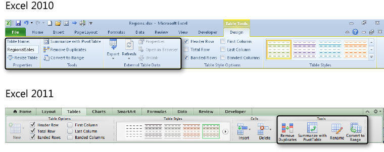
A handful of data-related features are also offered for tables, some more significant than others, as shown in Figure 18-9. In Excel 2010, these tools are located on the first half of the Table Tools Design contextual tab. In Excel 2011, they’re on the last half of the Tables tab.
If you intend to reference the table in formulas or with other functionality (such as macros), it’s a good idea to change the table name to something more intuitive that describes the data in the table. Otherwise, there’s nothing wrong with leaving the default name.
In Excel 2010, Resize Table enables you to redefine the cell range for the table. Note, however, that it’s usually quicker and easier to drag from the bottom-right corner of the table to do this, as explained in Chapter 17.
In Excel 2010, the Summarize With PivotTable option in the Tools group on this tab does the same thing as selecting PivotTable from the Insert tab. In Excel 2011, this option creates a manual PivotTable (that is, a PivotTable in which you need to add the fields to the correct areas), whereas the PivotTable command on the Data tab gives you the option to do the same or create an automatic PivotTable (one in which Excel adds suggested field placement for you).
Note
See Also To learn about creating and working with PivotTables, see Chapter 21.
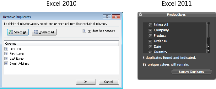
Remove Duplicates, which is new in Excel 2011, is available in the Tools group and does exactly what it sounds like. In the Remove Duplicates dialog box, shown in Figure 18-10, you see a list of column headings. Select only those columns in which you want to check for duplicate values. When duplicates are found, the entire applicable row will be deleted. Note that you can find this option on the Data tab as well, where it can also be used with worksheet ranges not formatted as tables.
Note
In Excel 2010, there isn’t any indication of found duplicates prior to them being removed. After you click OK, a message displays the count of duplicates that were found and removed. In Excel 2011, duplicate values are instantly indicated in the workbook and the total number found is displayed in the dialog box, as shown in Figure 18-10.
Convert To Range, the last option in the Tools group, is unlikely to be something you need often, but it’s nice to have it there when you do. This option strips all table functionality. Formatting from the table style remains, but it becomes direct cell formatting.
Note
See Also For help with table formatting if you choose to turn that range back into a table, see the upcoming sidebar, Table Style Isn’t Visible After Converting a Range to a Table.
In Excel 2010, the External Table Data group primarily provides options discussed in the final section of this chapter, Using External Data. However, it’s worth noting here as a nice shortcut for exporting the table to a Microsoft Office Visio 2010 PivotDiagram, available under the Export options.
Note
Companion Content For details on the outrageously cool PivotDiagram feature, see the article “Visualizing Data with Excel and Visio,” available in the Bonus Content folder online at http://oreilly.com/catalog/9780735651999.
How Can I Sum Only the Visible Cells in my Range?
When you have hidden rows or columns within a data range, functions can be frustrating because most of them include hidden cells when calculated. In fact, for earlier versions of Excel (specifically, Excel 2002 or earlier), the Microsoft Knowledge Base contains an article that provides a macro for summing only visible cells.
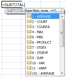
However, you can do this much more easily in recent versions by using the function number argument of the SUBTOTAL function. You can use the SUBTOTAL function to perform 11 different common functions on a specified data range, either with or without hidden cells included.
For example, the function number to sum only visible cells is 109. So, the formula =SUBTOTAL(109,A1:A25) provides a sum of visible cells in the range A1:A25.
In Excel 2010, after you select the SUBTOTAL function from the Formula AutoComplete list, you get a subsequent list of function numbers from which to select, as shown in Figure 18-11.
Ever wonder what the difference is between a function and a formula? It might appear that Excel uses the terms interchangeably, but it really doesn’t. A function is an action that you want to perform. A formula is the entire expression you create, including the function and the related arguments that you supply.
For example, SUM is a function; =SUM(A1:A25) is a formula.
This section looks at Excel functions in general, from accessing the function you need to referencing data, nesting functions, or auditing formulas.
There’s very little that Excel can’t do when it comes to working with data. More than 300 built-in functions are available from the Formulas tab, providing a much broader range of actions than most Excel users realize, including many functions that aren’t mathematical calculations at all.
In Excel 2010, the Function Library group on the Formulas tab does a nice job of exposing them all, and makes it easy to figure out which function you need. When you select a function from this group, the Function Arguments dialog box opens to help you complete the arguments for your formula.
Note that you can also click Insert Function on the Formulas tab to open the Insert Function dialog box, where you can select a function and see its description. When you click OK, the Function Arguments dialog box opens to help you complete the formula.
In Excel 2011, you can access the list of functions on the Formulas tab, under the Insert button. Or, also on the Formulas tab, click Formula Builder for a pane that provides information about your selected function and helps you complete the arguments.
Note that you can also access the Formula Builder from the Formula Bar (click the Function icon), from the Standard toolbar (click the Toolbox icon), or from the Insert menu (click Function).
In Excel 2010, when you point to an option under any of the headings in the Function Library, you get a ScreenTip showing a description of the selected function, such as with the CONCATENATE function shown in Figure 18-12. In Excel 2011, the Formula Builder (also shown in Figure 18-12) provides the same information directly below the list of functions.
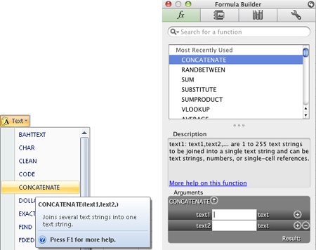
Figure 18-12. The Function Library in Excel 2010 (left) and the Formula Builder in Excel 2011 (right) provide similar tools to help you easily create the formulas you need.
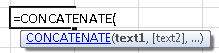
CONCATENATE is a good example of the fact that there’s also much more you can do with many functions than you might expect at first glance. The description you see in Figure 18-12 gives you a basic idea of when you might want to use that function. To insert a function in Excel and get help along the way, do one of the following.
When you open the Formula Arguments dialog box (Excel 2010) or the Formula Builder (Excel 2011) as noted earlier, you get a list of arguments to help you complete the formula.
In the CONCATENATE example, the dialog box in Excel 2010 adds space for more strings as you need it.
In Excel 2011, to add more strings, click the plus (+) button to the right of the text box. (Notice that the Formula Builder also provides more information about the function, such as the fact that you can use CONCATENATE to join up to 255 strings.)
Even with all of this help, these tools don’t tell you everything you might need to know to get the most out of the function. In the CONCATENATE example, you might want to know that you can use other functions in your formula as individual strings, or that you can use an ampersand (&) as an operator to join text strings instead of using the CONCATENATE function name.
Fortunately, help on Excel functions is hands-down the best built-in help available in any Microsoft Office program, and there are a few easy ways to access it.
You can access Help right from the Insert Function (or Function Arguments) dialog box or the Formula Builder pane to get much of this information, including examples. To do this in Excel 2010, click the link named Help On This Function. In Excel 2011, the link is named More Help On This Function.
If you’re typing your function or selecting it from the AutoComplete options, the fastest method for getting help is to use the hyperlink in the function argument ScreenTip, shown in Figure 18-13. (In Excel 2010, you won’t know the hyperlink is there until you point to the function name in the tip.)
Both Excel 2010 and Excel 2011 also provide a Help page with a complete list of built-in worksheet functions by category, including hyperlinks to the help articles for each. To access this list in Excel 2010, point to a function in the Function Library and then press F1. In Excel 2011, on the Formulas tab, in the Function group, click Reference.
Of course, you can also press F1 at any time to open Help in Excel 2010 or, in Excel 2011, click the Help icon on the Standard toolbar. Then type the function name into the search box.
Detailed help exists for most functions, including explanations of each argument and, in many cases, examples that you can copy and paste into a worksheet.
Note
If the hundreds of built-in functions and the various ways in which you can use many of them don’t give you what you need, you can find even more or write your own custom functions using Microsoft Visual Basic for Applications (VBA). (Check out the WorksheetFunction object in Excel VBA for a few built-in functions that don’t appear on the Formulas tab.)
Note
See Also To learn how to get started working with VBA, see Chapter 23.
The only limitation to using functions is that you have to understand enough about what the function is intended to do to be able to complete it effectively. When you aren’t completely clear on a particular argument required by a function, in Excel 2010, use the Function Arguments dialog box to complete the formula. In Excel 2011, use the Formula Builder.
If you’ve started to type the function or selected it from an AutoComplete list, in Excel 2010, on the Formulas tab, click Insert Function to open the Function Arguments dialog box. In Excel 2011, on the Formulas tab, click Formula Builder (or use another access point, as previously described, to open this pane).
When your insertion point is in a cell that contains a function and/or function arguments, the Function Arguments dialog box or the Formula Builder will automatically be set up for that function and reflect any arguments you’ve already provided.
Note
Because the Formula Builder in Excel 2011 is part of the Toolbox, Mac users can leave the Formula Builder open to get assistance on any function at any time.
Exploring Function Improvements
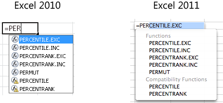
For the engineer, scientist, and financial analyst readers, the most exciting news for functions is that over 45 statistical, financial, and mathematical functions have been improved. Some functions have been renamed to more accurately reflect what they do, and there are also new versions of functions that better align with statistical, industry, and scientific definitions and give you increased compatibility across platforms. For example, the PERCENTILE.INC function was added to be more consistent with industry expectations. Here are a few items to keep in mind for these function improvements.
Improvements to functions are automatic—you don’t need to do anything different when using an improved function. As a matter of fact, when you open a workbook created in a previous version, any improved functions will automatically recalculate.
If you share workbooks with users of previous versions of Excel, older versions of the functions are still available to maintain compatibility. When you’re using Formula AutoComplete, available compatibility functions are identified, as shown in Figure 18-14.
Prior to sharing workbooks with users of a previous version, use the Compatibility Checker to find out whether your workbook uses a new or renamed function.
To do this in Excel 2010, click the File tab and then click Info. Under Check For Issues, click Check Compatibility.
In Excel 2011, on the View menu, click Compatibility Report. Or, in the Toolbox, click the Compatibility Report icon (the rightmost icon on the bar at the top of the toolbox).
Note that you can easily access a complete list of compatibility functions. See the Compatibility category in the Function Library (Excel 2010) or the Formula Builder (Excel 2011).
If you remember that a function is just an action and a formula is what you use functions to create, it’s easy to see how you might expand the capabilities of your work with functions by using multiple functions together within a single formula.
To use a function as an argument of another function, you need to know only these two points:
Type the function name and its arguments—do not put an equal sign before the name of the nested formula. Only the outermost formula starts with an equal sign.
Depending on the syntax of your formula, you might need to place parentheses around the nested formula, just as you would place parentheses around an individual operation in any formula to control the way the formula calculates. However, other characters (such as quotation marks) are never used around a nested formula.
Figure 18-15 provides a simple example of a nested formula. This formula reads as follows:
If the sum of A19 and A20 is greater than or equal to the average of A21 and A22, the value is true. Otherwise, the value is false.
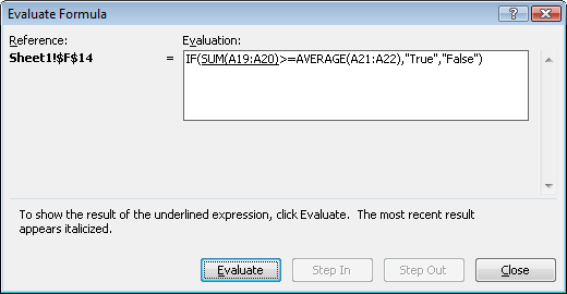
For Excel 2010 users, to confirm the logic in your nested formula—that is, to confirm that the formula is calculating nested formulas in the order you want—use the Evaluate Formula tool. To do this, select the cell containing the formula to evaluate and then, on the Formulas toolbar, in the Formula Auditing group, click Evaluate Formula.
In the Evaluate Formula dialog box (shown in Figure 18-16 for the sample nested formula shown in Figure 18-15), click Evaluate to see the results of the underlined portion of the formula. Continue to click Evaluate to view the order in which Excel completes the calculation.
Note
When you use defined names or structured references (discussed in the following section of this chapter), Evaluate will first show the cell range indicated by the reference and then show the result of the applicable calculation.
For Mac Users
Even though you don’t have the Evaluate Formula tool, you can get similar results with the Formula Builder. Although it won’t display the exact calculation order, it will display the result of each formula argument along with the result of the formula. And—unlike the Function Arguments dialog box in Excel 2010—you can place your insertion point in any nested function in the Formula Bar, and the Formula Builder will display the arguments and result of each argument for that function, as shown in Figure 18-17.
When you’re writing nested formulas in Excel 2011, to access the AutoComplete list after adding the outermost function, press Ctrl+Option+down arrow.
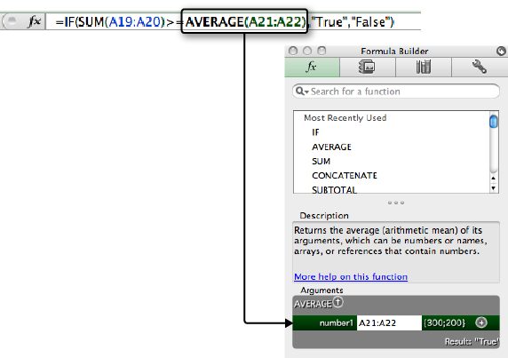
![]() Notice the arrow next to the function name in Figure 18-17, also shown at left. Clicking that arrow will take you back to that argument’s parent function. For example, in Figure 18-17, clicking the arrow will take you back to the IF function and its arguments.
Notice the arrow next to the function name in Figure 18-17, also shown at left. Clicking that arrow will take you back to that argument’s parent function. For example, in Figure 18-17, clicking the arrow will take you back to the IF function and its arguments.
Naming in Excel refers to naming cell ranges for use as structured references. As introduced in the section Using Tables As a Data Tool, earlier in this chapter, a structured reference is a reference to a named range rather than a cell range. The purpose of using names is so that you can simply update the cell range included in the defined name, and any references to that name throughout the workbook automatically update.
For example, say that you name the range C1:C10 as C_range and use that in several formulas, such as =Average(C_range). If you later need to include more data in that range and you redefine C_range to include C1:C18, all formulas that reference that range will update accordingly.
To quickly name a cell range, start by selecting the range. Then, in the Name Box on the Formula bar, shown in Figure 18-18, type the name you want to use for the range and press Enter. Names can contain only letters and numbers, and can’t include spaces.
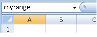
By default, a new name will be recognized throughout the workbook, so that you can reference a range on one sheet from a formula on another sheet without having to specify the source worksheet. To make the named range local only to the active worksheet—so that you can use the same name for ranges on more than one sheet in the same workbook—before the range name, type the sheet name followed by an exclamation point.
For example, type myrange as a range name that will be recognized throughout the workbook, or Sheet1!myrange to have the same range name recognized only on Sheet 1. To avoid confusion in your formulas, don’t duplicate range names—except in cases where the duplicated range names would be intuitive to all workbook users.
Instead of creating ranges using the Name Box, you can use the New Name dialog box (called Define Name in Excel 2011). In the New Name dialog box in Excel 2010, you can select the scope for the reference (workbook or active worksheet) and add comments about the range.
In Excel 2010, you can also use the Name Manager dialog box to see all defined names and table names throughout the workbook. Access this dialog box, shown in Figure 18-19 on the Formulas tab, in the Defined Names group.
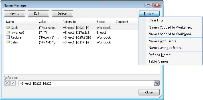
Just select a defined name to edit its range in the Refers To box at the bottom of the dialog box. When you’ve finished making changes, click the check icon to accept the changes.
You can also select a name and then click Edit to change the name, comments, or cell range of a defined name, or the name of a table. Note that the scope of a defined name can’t be edited.
Click Filter to limit your view by local or global name, table or defined name, or names containing errors.
Note
In both Excel 2010 and Excel 2011, if you change the name of a range or a table, any references to that range or table will automatically update with the new name. However, references to renamed items in other workbooks will update only if both workbooks are open at the same time. If the workbook containing the reference isn’t open when you change the referenced name, an error may occur when you next open the workbook in which the reference resides.
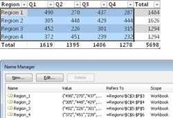
Excel also provides a nice tool for naming several ranges at once. For example, if you want to create defined names for individual table rows, start by selecting the data to include in the range along with the row headings, such as you see in the top portion of Figure 18-20. Then do the following:
In Excel 2010, on the Formulas tab, in the Defined Names group, click Create From Selection. In Excel 2011, on the Insert menu, point to Names and then click Create.
In the Create Names From Selection dialog box (Create Names dialog box in Excel 2011), select Left Column (in this example) as the source from which to create the names.
When you do this in Excel 2010, the resulting names and their respective ranges are shown in the Name Manager, as you see at the bottom of Figure 18-20. Notice that the cells used for the defined names are not included in the ranges.
In Excel 2011, you can verify your named ranges in the Define Name dialog box. To do this, on the Insert menu, point to Names, and then click Define.
As introduced in the section Using Tables As a Data Tool, earlier in this chapter, when you create a formula that references certain parts of a table, such as an entire column of data, the totals row, or all data in the table, you can use structured references to that table content. Structured references enable formulas to automatically adjust for changes in the table data range.
Table 18-1 lists the portions of the table that you can reference this way, along with the correct reference. Find examples and instructions for using these references in Table 18-2 and the tips that follow.
Table 18-1. Syntax of structured table references
Table component | Reference |
|---|---|
The entire table | Table name |
Any column | Column heading name surrounded by brackets, such as [Q1] if the first column name is Q1 |
All data | [#Data] |
Column headings | [#Headers] |
The total row | [#Totals] |
The active row | [#ThisRow] |
All contents of the specified table or column, including header and total cells if they contain applicable values | [#All] |
Note
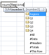
For the examples of structured references that follow in Table 18-2, refer to Figure 18-21, which depicts a table named Regions. SUM formulas are used for all examples.
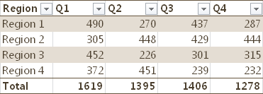
Table 18-2. Using structured references with tables
Keep the following rules in mind to create structured references:
When using references inside the table, such as in calculated columns, you don’t need to specify the table name. Outside the table, always specify the table name.
Type brackets around each element of a structured reference other than the table name, as well as brackets around an entire expression that refers to a single specific portion of the table.
Use a comma between any of the five special-item identifiers (those options that start with the pound sign) and the range to which they refer.
Use formula operators as you would in standard ranges, such as [Q1]:[Q3] to refer to columns Q1 through Q3. Use [Q1],[Q3] to refer to columns Q1 and Q3. Note, however, that only contiguous ranges (those that use a colon) can be qualified by a single special-item identifier.
[#ThisRow] doesn’t do exactly what you might think, because table rows can’t actually be specified as structured references. This option can apply only to specified cells in the active row, so it always must be used with column identifiers. For example, =Regions[[#ThisRow],[Q1]] refers to the cell in the active row in column Q1.
So, what do you really have to know among all of the structured reference options discussed in this section? Not as much as you’d think. In fact, the preceding bullet points are pretty much all you need to remember, because Excel will create structured references for you when you select various table components while building a formula. For example, if you select the entire table column, your formula will use a structured reference instead of a cell range that includes cell addresses. The main thing to keep in mind is if you want your formulas to automatically accommodate changes in a table, you need to use structured references in your formulas, not cell addresses.
For those who prefer to type their entire formula, AutoComplete for formulas offers help for working with structured table references. When you start typing a reference either directly in a cell or the Formula bar, you’ll see the available AutoComplete options. For example, working from the sample table data shown earlier in Figure 18-21, here’s how to use AutoComplete to add a structured reference as the range for a SUM function.
Type =SUM(R and you’ll see AutoComplete with function names that start with R, as well as the table name.
In Excel 2011, after you type the text shown in step 1, press Ctrl+Option+down arrow to access the AutoComplete list.
Scroll to Regions in the AutoComplete list and press the Tab key to apply it to your formula.
Next, type a single open bracket after the table name if you just want to reference a portion of the table, or type two consecutive open brackets if you’re going to use a special-item identifier along with a specified portion of the table. AutoComplete will again show you available options for the specified table and specified syntax, such as you see in Figure 18-22.
If the option you want isn’t available, check your syntax (for example, you might need an additional bracket, or a comma between references).
You have a complex workbook with multiple tables on multiple worksheets and many formulas throughout. When one calculation leads to the next, which leads to the next, the last thing you need to see is an error result. You have nested formulas, array formulas, structured references—and one small error in just one of those components can cause a domino effect of errors to ripple throughout your workbook. How do you even begin to track down the culprit? Better yet, how do you put controls into your formulas to prevent those error messages in the first place? Let’s take these two questions one at a time.
When an error occurs in a cell, you have several options to help you quickly resolve the issue, as follows.
When you select a cell containing an error result, an Error Options button appears. When you point to the icon at left, you can click the arrow that appears beside it to access tools for working with the error, such as a shortcut to the online help topic for that error type and other options. In Excel 2010, you’ll also see the option Show Calculation Steps, which opens the Evaluate Formula dialog box discussed earlier in this chapter.
Determining the source of the error might be as easy as clicking in the Formula bar when the error cell is selected, because you will see all referenced cells or ranges highlighted on the active sheet. If you understand the type of error, this might be enough information to quickly get you to the result you need. Of course, if some references are to ranges outside the active sheet, those won’t be highlighted on screen.
When you have more than one error on the sheet, in Excel 2010, on the Formulas tab, in the Formula Auditing group, click Error Checking. In Excel 2011, on the Formulas tab, in the Audit Formulas group, click Check For Errors. The dialog box that opens provides options similar to an Error Options button, as well as Previous and Next buttons to let you move through all errors on the sheet.
To trace the source of the error for the selected cell, click the arrow beside Error Checking (Check For Errors in Excel 2011) and then click Trace Error. Precedent arrows will appear, showing all available referenced cells in the error formula.
When using precedent or dependent arrows, notice that precedent arrows for off-screen references (such as source data on other sheets or in other workbooks) appear as a dashed line leading to a worksheet icon. Double-click the dashed arrow to open the Go To dialog box, in which you’ll see the location of the source range. Note, however, that if the source range is in a separate workbook, that workbook must be opened to access it using this method.
When the answer isn’t obvious to you, in Excel 2010, using Evaluate Formula is the easiest way to see the source of the error. Each time you click the Evaluate button, you see the next step in the formula, until the error occurs, so you can quickly and clearly see which argument caused the error. In Excel 2011, use the Formula Builder as shown earlier, and you’ll see the error result next to the argument causing the error.
Note
In previous versions of Excel, you need to use a named range to reference other worksheets in your validation rules. Now you can reference a worksheet directly and skip the named range step. However, to accommodate worksheet changes, using a named range is still considered best practice.
Caution
When you save your workbooks to the cloud, note that (as of when this book was written) you cannot view or edit workbooks that contain data validation in Excel Web App. Using either Excel 2010 or Excel 2011, save a copy of the workbook without the data validation rules to view and edit it online.
However, as noted in Chapter 2, note that Microsoft Office Web Apps are a new suite of programs that are in their first version as of this writing. So, if you wonder if that limitation has changed by the time you’re reading this, give it a try. You won’t harm your file by trying to view or edit it online. If you receive an error message, you can then just open the workbook in Excel on your computer to remove validation rules.
Note
See Also To learn about Excel Web App capabilities and limitations, see Chapter 2.
Of course, preventing errors is an even better solution than troubleshooting them. It’s certainly not always possible to control the worksheet to that extent, and not necessarily even appropriate in all cases, but using the Data Validation tool can be a great help.
Say, for example, that data entered into certain cells must be whole numbers between 50 and 80, or an error will result in formulas that are dependent on those cells. You can select the cells that require those values and set up data validation that informs users of the type of values required. You can even stop users from entering other types of values.
To do this, start by selecting all cells that require the same validation. Noncontiguous ranges can be used (to include noncontiguous cells, hold the Ctrl key—the Command key in Excel 2011—while selecting). Then, do the following:
On the Data tab in the Data Tools group, click Data Validation (Validate in Excel 2011).
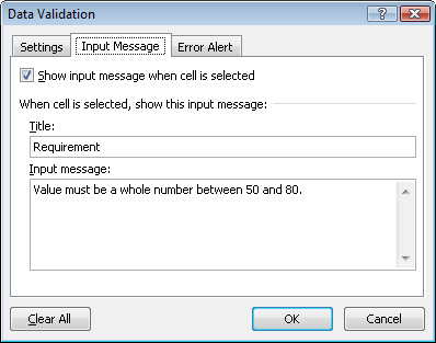
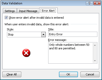
In the dialog box that appears, complete the settings you want on the Settings, Input Message, and Error Alert tabs, as shown in Figures Figure 18-23 through Figure 18-25.
Note that the example shown in the referenced images uses the preceding scenario that requires whole numbers between 50 and 80.
Figure 18-23. On the Settings tab, specify criteria for data entered into selected cells. Actions on the other two tabs of this dialog box are ignored if no criteria are set on this tab.
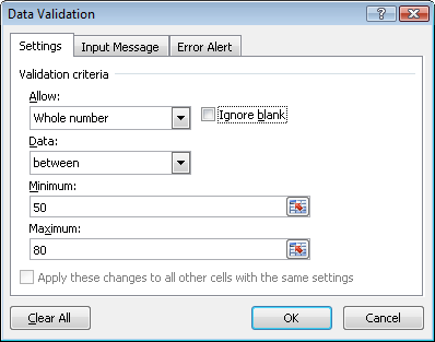
Notice that you can’t add an input message or an error alert without first specifying data validation criteria. However, you are not required to use both an input message and an error alert action when you use data validation. So, you might choose to use this feature to prevent errors or just to provide guidance to users on preferred types of data.
Note
When you turn off the Ignore Blanks option on the Settings tab, you have some control over blank cells but not complete control. If the user clicks in a cell and deletes all content, any error action will be taken. However, if a user selects the cell and presses Delete, the content of the cell will be deleted without any error alert.
Caution
Following are two important considerations for working with data validation:
When you use the fill handle or otherwise copy content from one cell to another, data validation settings are copied as well. So, if you fill a cell for which validation is active with invalid data from another cell that has no validation, data validation will be removed from the destination cell.
In Excel 2011, at the time of this writing, if your data validation rule is in a table, it may not be carried over to newly added rows, so you’ll need to add it again. The easiest way to do this is to select a cell that includes your data validation and any cells that need it added. Then, on the Data tab, click Validate, and you’ll be prompted to extend data validation to those cells. When you click OK, the Data Validation dialog box displays. Just click OK once more to accept the current settings, because your existing rule is picked up from your selection.
When you use Excel, you’re working in an environment designed for logic and clarity. Excel is a spreadsheet, after all—no matter what kind of great formatting you use in your workbooks, the concepts of Excel remain black and white. So, for best results whenever you create Excel documents or use Excel to create content for other documents, let the logic of Excel work for you.
Keep in mind that something as simple as the Freeze Panes feature on the View tab (Layout tab in Excel 2011) can help you review your worksheet data more effectively. Or, in Excel 2010, when you need to keep an eye on a few specific, important cells in any open workbook, regardless of which open workbook is active at the time, use the Watch Window (available from the Formula Auditing group on the Formulas tab).
Note
When your data range is formatted as an Excel table, you have an organization tool available that is even easier to use than Freeze Panes. Notice that if you scroll down in the table so that the table headings move past the top of the screen, the sheet column headings automatically take on the table column heading names. And, as previously mentioned, in Excel 2010 the filter and sort options remain at the top of the columns as well.
Also look for friendly solutions that can streamline your work while remaining intuitive to other users of the workbook. For example, before you hide columns or rows, consider whether the Outline feature would be more effective. Using the Outline options on the Data tab, you can group selected cells so that you can expand or collapse portions of your workbook as needed. When you group cells using the Outline feature, a pane appears at the left or at the top of your worksheet (depending on whether you have grouped rows or columns) with guidelines showing the grouped range and a minus icon that you can click to collapse that range. When collapsed, the icon becomes a plus sign that you can click to again expand that range. Using this feature can allow you to easily hide cells when you don’t want to view or print them, but the pane that shows the outline makes it clear to any user that the worksheet includes hidden cells.
Note
The Subtotal tool that you see on the Outline group of the Data tab in Excel 2010 (or on the Data menu in Excel 2011) is not available for ranges formatted as tables. However, when you hide cells (or collapse grouped cells), remember that by default the total row of a table automatically uses SUBTOTAL formulas that include only visible values. For an explanation of SUBTOTAL function behavior and options, see the section Using Tables As a Data Tool, earlier in this chapter.
Also remember that tasks that might sound complex don’t always need to be. For example, though PivotTables are simpler than you may think, you might need just an AutoFilter for the information you want from your data.
In fact, filters and sorts are incredibly flexible, with features such as the ability to sort and filter cells by color, and quick filters that build common filter criteria for you. Sort & Filter options are available on the Data tab and, in Excel 2010, on the Home tab as well.
To create a custom sort (such as sorting by cell or font color) in Excel 2010, on the Data tab, in the Sort & Filter group, click Sort. Or, on the Home tab, in the Editing group, click Sort & Filter and then click Custom Sort. In Excel 2011, on the Data tab, in the Sort & Filter group, click the arrow next to Sort, and then click Custom Sort.
Use the Sort dialog box, shown in Figure 18-26, to add the sorting rules you need.
Depending on the sort type you select, you’ll get different options. When you sort on Cell Icon, for example, you can select which icon, out of those available in the range, to sort at the top or bottom of the list, as shown in Figure 18-26. Notice also that you can copy a sort level to duplicate the settings and then change just what you need. This is particularly handy when you want to sort by color or icon and specify the order for more than just the first or last values in the list. Remember that sorts will execute in the order in which the sort levels appear in this dialog box.
To apply a filter, on the Data tab, in the Sort & Filter group, click Filter. Or, in Excel 2010, on the Home tab, in the Editing group, click Sort & Filter and then click Filter.
Both of these actions apply an AutoFilter arrow to the column headings in your selected range. (When working in a range that’s formatted as an Excel table, remember that the AutoFilter arrows are automatically applied to your column headings by default.) When you click an AutoFilter arrow, you get filter options as well as another access point for sort options, as you see in Figure 18-27.
Notice that the Excel 2011 options appear in an independent pane that you can move on screen as needed.
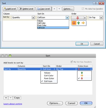
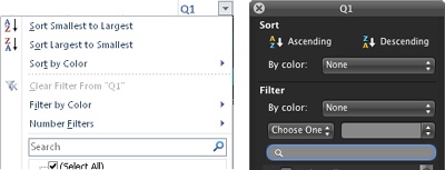
Figure 18-27. AutoFilter options for sorting and filtering, shown in Excel 2010 (left) and Excel 2011 (right).
The Sort By Color and Filter By Color options include fill color, font color, or icons, as applicable to the selected range. Note that colors that are part of a table style do not appear as available options for sort or filter by color, as those colors are applied automatically based on content position in the table rather than the content itself.
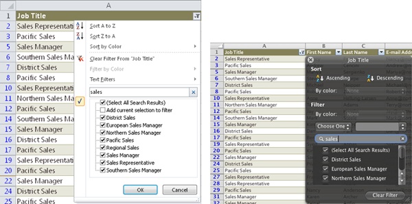
One of my favorite new features for filters is the instant search. Never again do you need to endlessly scroll through a long list of choices. Just type your search string in the search box, and Excel will instantly show you all items that match your search string, as shown in Figure 18-28.
And, for Excel 2010 users, after you perform an instant search, check out the Add Current Selection To Filter option, shown at left in Figure 18-28. You can use this option for subsequent searches to add filter items and maintain your previously filtered list.
Note
For Excel 2011 users who want to try the tip in the preceding sidebar, you can also use Command+End (as an alternative to Ctrl+End) to move your insertion point to the end of the used range. Excel 2011 gives you the option to use many Excel for Windows keystrokes available, so the Ctrl and Command keys are interchangeable—especially for some file management, editing, and navigation commands. For example, you can use Ctrl+O in Excel 2011 to open a file, Ctrl+C to copy a selection, and Ctrl+Home to move your selection to the top of the sheet or object. But this option is not universal. So, if the Ctrl key doesn’t give you the result you expect for a keyboard shortcut, try the Command key.
When your source data isn’t in an Excel workbook, have no fear. It’s quite easy to import data from a number of sources, and even in many cases to keep that data linked to a dynamic source so that it updates automatically when needed. Following is a summary of common data types you may want to import and their related options. In Excel 2010, find all of these options on the Data tab, in the Get External Data group. Excel 2011 includes some similar options, available on the Data tab in the External Data Sources group.
When you import data from a database in Excel 2010 or Excel 2011, you select the database that contains your source data, and Excel prompts you to select a table within that database, if it contains multiple tables. Once you select the data source, you get the option to import the data into a table, PivotTable, or (in Excel 2010) PivotTable and PivotChart.
Note that, even if you want to create a PivotTable, it’s a good idea to import the data as a table. You can create a PivotTable (or, in Excel 2010, a PivotChart) from the table in just a click, and you get quicker access to the source data.
When you import data from text, your source file can be a .txt or .csv file type. (Note that the .prn file format can be used as well, but your files must be space-delimited text files, not printer files.) Data imported from a text source (such as text delimited with commas between fields in a record) will be imported into an unformatted range. Like other data types, data from a text source will remain linked to its originating file by default. However, you will be prompted to select the file from which to get data whenever you click Refresh. For this reason, when you have multiple imported text ranges, refresh them one at a time rather than all at once to ensure that the correct data is refreshed to the correct range. To refresh the selected range instead of all connections at once, right-click in the range and then click Refresh. Or, in Excel 2010, on the Data tab, click the arrow below Refresh All and then click Refresh. In Excel 2011, from the Data menu, click Refresh.
When you choose the option to import data from the web (Excel 2010 only), you get a window in which you can browse to the webpage you need. Excel can import table content from a website, so an arrow will appear beside each table on the selected page that can be imported. You can select as many as you need. Just click the yellow arrows to place a check box by each table you want to import. After you click Import and choose the location for your content, you’ll see a line of text indicating that Excel is getting the data, and it will populate as many cells as needed to provide the data you requested.
Note that although Excel 2011 does not include the feature to import from the web, you do have the option to import data from an HTML file. So, you can save a webpage as an HTML file and then import the content you need.
Caution
With any type of imported data, when selecting a location for that data, be sure to leave enough room between the imported content and any other existing data on the sheet. If the imported data would overwrite an existing range, Excel may attempt to move the data, but it might copy unwanted formatting when it does. Alternately, Excel might refuse the operation. If the operation is refused, but a single cell is available where you indicated to place the imported data, the text string that indicates what data is being imported will appear. Though it looks like static text, it’s not. Move that string to a location on the sheet with ample space for the imported data and then, on the Data tab, click Refresh All to finish importing the data.
For any imported data type, note that you can set several custom properties, such as how and when the data refreshes. To access these options, click in the external data range and then do the following:
In Excel 2010, on the Data tab, in the Connections group, click Properties.
In Excel 2011, on the Data menu, point to Get External Data, and then click Data Range Properties.
Note that available options vary based on the type of data source.