

Performance test with a Cognos BI example
With the new technologies such as parallel vector processing, core-friendly parallelism, and scan-friendly memory caching, the DB2 with BLU Acceleration feature optimizes the best use of the hardware in your existing infrastructure for analytics. With adaptive compression and data skipping capabilities on columnar store, BLU Acceleration provides another level of performance for complex analytic workloads.
After a BLU Acceleration deployment, you might be eager to test the immediate performance gain that BLU Acceleration can provide to your analytic workloads. Although users are open to using their own testing tools, in this chapter, we demonstrate a built-in DB2 utility and a Cognos tool (specific for Cognos users) that you might find helpful to measure your query performance for testing or evaluation purposes.
Although this chapter uses Cognos BI workloads as an example, DB2 with BLU Acceleration can also benefit other analytic workloads generated by other business intelligence vendors.
The following topics are covered:
5.1 Testing your new column-organized tables
Testing is an essential and important phase in a deployment project. After you convert, load, or replicate your data into an analytic-optimized column store in DB2, you might be excited to experience the performance gains and storage saving for your environment. Users can use their own favorite benchmarking tool for testing their workload performance before or after their BLU-deployment. A helpful alternative is to use the built-in DB2 utility or a Cognos BI tool to help you measure performance results of your workloads.
In 5.2, “DB2 benchmark tool: db2batch command” on page 171, we use the built-in db2batch command to quickly demonstrate the performance comparisons of our Cognos BI workload, against original row-organized tables and the new BLU column-organized tables. In 5.3, “Cognos Dynamic Query Analyzer” on page 175, we perform a similar comparison with Cognos Dynamic Query Analyzer.
Besides the db2batch utility, DB2 also includes a variety of monitoring metrics that you can also use for determining query run times. For more details about these monitoring metrics, or for observing storage savings and compression rates of your new BLU column-organized tables, see Chapter 6, “Post-deployment of DB2 with BLU Acceleration” on page 187.
|
Note: Performance measuring results illustrated in this chapter are for functional demonstration only. They are not being used as a benchmarking reference.
|
5.1.1 Scenario environment
Here we describe the lab environment for the examples used in this section.
Hardware used in our scenario
One of the many advantages of BLU Acceleration technologies is that acquiring new hardware to run BLU is unnecessary. For best performance, we advise you to follow the suggested hardware from 2.4, “Prerequisites” on page 20. For this book, we used an existing System x3650 with non-solid-state drives (non-SSDs) available in our lab to complete our functional scenario. The system had less than the minimum memory recommended for the number of cores in it. Even without the SSDs and the recommended memory requirements, we observed a 6 - 20 times improvement in query response time during the test.
Sample workload used in our scenario
The workload we used in this example is mainly composed of six GO Data Warehouse Sales queries from the Cognos Dynamic Cubes samples pack, as illustrated in Figure 5-1 on page 171. These Dynamic Cubes samples are based on the sample database model from the Cognos sample GS_DB database. In our example, our sales fact table, GOSALESDW.SLS_SALES_FACT, is expanded to 3,000,000,000 (three billion) rows for the sole purpose of this functional demonstration.

Figure 5-1 Sample queries used in this example
For more details about the IBM Cognos Business Intelligence Sample Outdoors samples and setup instructions, visit the following website:
5.2 DB2 benchmark tool: db2batch command
DB2 provides a db2batch command that is used for benchmarking SQL or XQuery statements in all editions. This built-in DB2 command takes queries from either a flat or a standard input. Then, it dynamically prepares the statements and returns the query results and the required time to run the provided statements.
Before and after loading the Cognos BI sample data into BLU column-organized tables, we run the db2batch command to capture the performance results of the captured Cognos sample query workloads, as demonstrated in Example 5-1.
Example 5-1 db2batch benchmark tool example
db2batch -d GS_DB -f DQworkloads.sql -iso CS -r results.out,summary.out
In Example 5-1, we specify several options for the db2batch benchmarking tool command:
-d GS_DB Specifies the name of the database (in our example, GS_DB)
-f DQworkloads.sql This input file contains the SQL statement to be run by the tool dynamically (in our case, DQworkloads.sql)
-iso CS Sets the cursor isolation level to cursor stability (CS for ODBC read committed). This determines how data is locked and isolated from other processes while being accessed. Another available isolation level is uncommitted read (UR)
-r results.out,summary.out
No spaces exist between the two file names and the comma.
Specifies the query results to be returned in the results.out file; and the performance summary to be returned in a separate file called summary.out
With a few options to the db2batch command, we can determine the performance information about the query workload on the database level.
|
Tip: To reduce impact of writing to disk during the performance benchmark, put a limit on the number of rows that should be written to the results output file. To do so, use the --#SET ROWS_OUT <#_of_rows_in_resultsfile> control option in the workload SQL input file. For more information, see the following web page:
|
Example 5-2 shows an excerpt of the DQworkloads.sql input file. The following control option is added to limit the number of rows written to the results output file:
--SET ROWS_OUT <#>
Example 5-2 Example workload SQL input file for db2batch
--#SET ROWS_OUT 10
SELECT "SLS_PRODUCT_DIM"."PRODUCT_BRAND_KEY" AS "Product_brand_Product_brand_key",
"GO_TIME_DIM2"."CURRENT_YEAR" AS "Time_Year",
SUM("SLS_SALES_FACT"."GROSS_PROFIT") AS "Gross_profit"
FROM "GOSALESDW"."EMP_EMPLOYEE_DIM" "EMP_EMPLOYEE_DIM1" INNER JOIN "GOSALESDW"."SLS_SALES_FACT" "SLS_SALES_FACT" ON "EMP_EMPLOYEE_DIM1"."EMPLOYEE_KEY" = "SLS_SALES_FACT"."EMPLOYEE_KEY" INNER JOIN "GOSALESDW"."GO_TIME_DIM" "GO_TIME_DIM2" ON "GO_TIME_DIM2"."DAY_KEY" = "SLS_SALES_FACT"."ORDER_DAY_KEY" INNER JOIN "GOSALESDW"."SLS_PRODUCT_DIM" "SLS_PRODUCT_DIM" ON "SLS_PRODUCT_DIM"."PRODUCT_KEY" = "SLS_SALES_FACT"."PRODUCT_KEY" WHERE "EMP_EMPLOYEE_DIM1"."EMPLOYEE_KEY" BETWEEN 4001 AND 4972 GROUP BY "SLS_PRODUCT_DIM"."PRODUCT_BRAND_KEY", "GO_TIME_DIM2"."CURRENT_YEAR";
SELECT ...
5.2.1 Before BLU-conversion results
In Example 5-1 on page 172, we ran a db2batch command to test the captured workload against the row-organized Cognos sample GS_DB database before our BLU Acceleration conversion. Example 5-3 shows a sample db2batch output from the query run against the row-organized database. From the db2batch output summary, we find the following approximations of time spent:
•Approximately 1398 seconds (approximately 23 minutes) were spent for each query.
•A total of approximately 8389 seconds (approximately 2.3 hours) was spent to complete all six queries in the captured workload.
Example 5-3 db2batch results against row-organized tables in our example
* Summary Table:
Type Number Repetitions Total Time (s) Min Time (s) Max Time (s)
--------- ----------- ----------- -------------- -------------- --------------
Statement 1 1 1355.823464 1355.823464 1355.823464
Statement 2 1 1612.169303 1612.169303 1612.169303
Statement 3 1 1352.828554 1352.828554 1352.828554
Statement 4 1 1340.276011 1340.276011 1340.276011
Statement 5 1 1339.085966 1339.085966 1339.085966
Statement 6 1 1388.847591 1388.847591 1388.847591
Arithmetic Mean Geometric Mean Row(s) Fetched Row(s) Output
--------------- -------------- -------------- -------------
1355.823464 1355.823464 100 10
1612.169303 1612.169303 11 10
1352.828554 1352.828554 91 10
1340.276011 1340.276011 35 10
1339.085966 1339.085966 575 10
1388.847591 1388.847591 20 10
* Total Entries: 6
* Total Time: 8389.030889 seconds
* Minimum Time: 1339.085966 seconds
* Maximum Time: 1612.169303 seconds
* Arithmetic Mean Time: 1398.171815 seconds
* Geometric Mean Time: 1395.036726 seconds
5.2.2 After BLU-conversion results
Example 5-4 on page 175 shows the sample output captured the performance information after the sample database GS_DB is converted to BLU column-organized tables. In our results, we find the following information:
•Each query completed in less than 300 seconds (less than 5 minutes) that would otherwise complete in 23 minutes.
•The fastest-performed query completed in 80 seconds against converted column-organized tables, as opposed to the same query taking 1612 seconds, being the longest-performed query before the conversion. This is approximately 20 times faster than querying from data stored in a traditionally OLTP-optimized row-organized platform.
•The entire workload of six queries took approximately 1337 seconds (approximately 22 minutes) that would otherwise take 8389 seconds (approximately 2.3 hours) to complete.
Example 5-4 db2batch results against column-organized tables in our example
* Summary Table:
Type Number Repetitions Total Time (s) Min Time (s) Max Time (s)
--------- ----------- ----------- -------------- -------------- --------------
Statement 1 1 298.558335 298.558335 298.558335
Statement 2 1 80.128576 80.128576 80.128576
Statement 3 1 234.080254 234.080254 234.080254
Statement 4 1 197.261276 197.261276 197.261276
Statement 5 1 266.079743 266.079743 266.079743
Statement 6 1 260.751941 260.751941 260.751941
Arithmetic Mean Geometric Mean Row(s) Fetched Row(s) Output
--------------- -------------- -------------- -------------
1355.823464 1355.823464 100 10
1612.169303 1612.169303 11 10
1352.828554 1352.828554 91 10
1340.276011 1340.276011 35 10
1339.085966 1339.085966 575 10
1388.847591 1388.847591 20 10
* Total Entries: 6
* Total Time: 1336.860125 seconds
* Minimum Time: 80.128576 seconds
* Maximum Time: 298.558335 seconds
* Arithmetic Mean Time: 222.810021 seconds
* Geometric Mean Time: 206.099577 seconds
With a simple db2batch command, we can obtain an overview of the run times for a given query workload.
5.3 Cognos Dynamic Query Analyzer
For Cognos BI developers, Cognos Dynamic Query Analyzer (DQA) can be a useful tool to measure and analyze query workload performance before and after a BLU Acceleration deployment. Cognos Dynamic Query Analyzer provides a graphical interface for reviewing Cognos query logs. Logs are visualized in a graphical representation format, helping you understand the costs and how the queries are run from the view of a Cognos query engine. Dynamic Query Analyzer is the main tool to visualize queries in Dynamic Query Mode, but it can also be used for reports that are not based on dynamic cubes.
In this section, we continue the performance review before and after our BLU Acceleration deployment using Cognos Dynamic Query Analyzer. For more details about the sample data set we used in our scenario, see “Sample workload used in our scenario” on page 171.
5.3.1 Quick configuration of Cognos Dynamic Query Analyzer
Before we demonstrate our query results in Dynamic Query Analyzer, several items must be set up:
•Enable log tracing on dynamic queries, so that when any user generates a report, a query log trace is also generated for later review.
•Specify several settings in Dynamic Query Analyzer to connect to the Cognos instance and pull the query logs from the Cognos server.
This is a simplified demonstration of the preconfiguration to use Dynamic Query Analyzer. For more details about configuring Dynamic Query Analyzer, see the following web page:
You can download Cognos Dynamic Query Analyzer from IBM Passport Advantage® or IBM PartnerWorld® Software Access Catalog.
Enable query execution trace in Cognos Administration
Use the following steps to gather log tracing for query requests run under a QueryService:
1. Log in as a Cognos administrator. In the Cognos Connection web interface (Figure 5-2). Click IBM Cognos Administration to launch the administration view.

Figure 5-2 Launching IBM Cognos Administration from Cognos Connection
2. In IBM Cognos Administration, select Status → System → <name of target Cognos Server> → <name of target Cognos dispatcher> → Query Service → Set properties, as shown in Figure 5-3.

Figure 5-3 Set properties for QueryService of the target Cognos server or dispatcher
3. In the Set properties panel, select Settings. Then, locate the Enable query execution trace property, and select the check box under the Value column, as shown in Figure 5-4 on page 178. This enables query execution tracing and gathers the log and trace information for all requests to this QueryService. When query execution tracing is complete, you can return to this panel and disable the same property.

Figure 5-4 Enable Query execution trace for designated QueryService
Cognos Dynamic Query Analyzer configurations
Follow these steps to set preferences in Cognos Dynamic Query Analyzer to connect to your current Cognos instance. If required, you can optionally set the default log directory URI to pull your query logs from a web server instead of a local file systems.
1. In Cognos Dynamic Query Analyzer, select Window → Preferences. In the left navigation pane (Figure 5-5), select Cognos Server. Enter your Cognos Dispatcher and Gateway URIs, then click Apply. This makes sure that Cognos DQA is connected to your current Cognos instance.

Figure 5-5 Dynamic Query Analyzer: set Cognos Server preferences
2. In our scenario, we access our Cognos query execution logs from the Cognos web server. Therefore, we can optionally set the logging folder URI in the DQA Preferences settings. Select Logs in the left navigation pane (Figure 5-6), then enter the web server path that contains your Cognos query logs in the Log directory URI field. Click Apply and OK when finished.

Figure 5-6 Dynamic Query Analyzer: set Logs directory URL preferences
5.3.2 Opening query execution trace logs in DQA
Before this step, our users ran a few Cognos reports from Cognos connection against our three billion rows expanded GS_DB database for testing purposes. Reports were run before and after the database was converted to use BLU Acceleration as a comparison.
After enabling query execution trace and setting up Dynamic Query Analyzer, we are ready to review the query trace logs generated by the reports that ran previously. Query trace logs are generated in the XQE directory in the Cognos log directory as the reports are run.
Use the following steps to review the query trace logs:
1. Launch Cognos Dynamic Query Analyzer. Click Open Log.
2. In the Open Log dialog (Figure 5-7), select the query log to open. In our scenario, we open our query logs from the Cognos web server that we setup earlier. Other open log source options include previously opened files, or local file directory.
In Figure 5-7, we open two sets of logs from the same query that we executed before and after the BLU deployment for a comparison review.

Figure 5-7 Open Log from web server URL
3. Dynamic Query Analyzer opens the selected query logs in several views similar to Figure 5-8. By default, the following views are shown:
– Summary: Displays the overview information including the data source type, and total time that is needed to execute the query.
– Query: Displays the full query statement being run.
– Navigation: Shows the execution tree of the query in graphical format.
– Properties: Displays the detailed properties of a selected node.
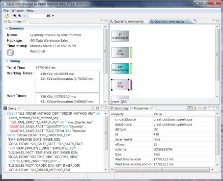
Figure 5-8 Dynamic Query Analyzer window-based views
5.3.3 Log summary before BLU Acceleration deployment
In our example, we focus on the timing Summary view of our query logs, specifically the performance numbers against the underlying database.
•Before converting the Cognos sample database to column-organized tables, the Quarterly revenue by order method query was run and query execution logs were captured. From the captured logs, Figure 5-9 shows the Summary trace of the relational data source component involved in the dynamic cube query. We observe that the total time spent in QueryService to fetch data from the source relational database is approximately 1,779,256 ms, which is approximately 30 minutes.
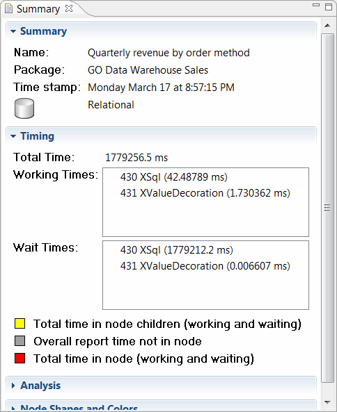
Figure 5-9 Timing summary against row-organized database
•You can review the logs in more depth and determine the actual time spent on querying the underlying database for a specific SQL component in the query. In the navigation view, click the Xsql node; the node details are displayed in the Properties view. The execution trace (Figure 5-10) shows that 91 rows were returned (nRows) from the SQL query. Overall, approximately 1779 seconds (approximately 30 minutes) were spent to complete the query against the source (row-organized) database.
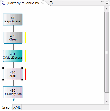
Figure 5-10 Xsql node and its properties against row-organized database
5.3.4 Log summary after BLU Acceleration deployment
After the Cognos Go Sales Warehouse database is converted into column-organized tables, we run the same sample dynamic cube Quarterly revenue by order method query. With Dynamic Query Analyzer, we review the log details. The sample outputs in this section are measured before any data is loaded in memory. Typically, you run the workload twice to experience the query response time when data is loaded in memory. In our scenario, reports returned instantly in the second run.
Figure 5-11 shows the timing summary for the relational data source component of the log, from the same dynamic cube query running against the converted column-organized tables. The log captured the total time spent querying from relational database at 277 717 ms, which is approximately 4.6 minutes. This is about 6.4 times faster than the same dynamic cube query against row-organized tables.
|
Note: This is a functional demonstration only, with workloads tested on hardware with less than minimum recommendations.
|

Figure 5-11 Timing summary against column-organized database
Again, we drill-down further to the same Xsql node properties that we reviewed previously for a direct comparison of SQL execution time from the database before and after BLU conversion. Figure 5-12 illustrates the Xsql node and its properties from a query that is executed after a BLU conversion. From the execution trace, we observe that the same SQL query completed in approximately 278 seconds on the database, returning 91 rows (nRows). This is 6.4 times faster than the same dynamic cube query against a row-organized database.

Figure 5-12 Xsql node and its properties against column-organized database
5.4 Conclusion
In this chapter, we demonstrated a DB2 benchmark utility and a Cognos tool that can be useful to measure workload performance before and after a BLU deployment for testing. Various other DB2 monitoring elements are available to perform a more thorough validation of a BLU Acceleration deployment. See Chapter 6, “Post-deployment of DB2 with BLU Acceleration” on page 187.
..................Content has been hidden....................
You can't read the all page of ebook, please click here login for view all page.