Recursion

Recursion is when a function calls itself. This seems like a recipe for disaster, but recursion is a powerful way to express some operations that are naturally defined in terms of themselves.

Another Binary Search

Consider the binary search introduced in Chapter 3, “Arrays and Algorithms”: You look at the midpoint of the range, and if that value equals the key, then you have succeeded. If the key is less than the middle value, you search the first half, and if the key is greater than the value, you search the second half. Finally, if the range is empty, you have failed. Note that this description of a search is defined in terms of searching! Here is a version of bsearch() that has no explicit loop. Instead, it calls itself to search either the first or the second half:

int bsearch(int arr[], int low, int high, int val)
{
    int mid = (low+high)/2;
    if (val == arr[mid]) return mid;  // success
    if (low == high)     return -1;   // failure
    if (val < arr[mid])               // keep searching...
       return bsearch(arr, low,  mid-1,val); // first half
    else
       return bsearch(arr, mid+1,high, val); // second half
}

Recursion must terminate at some point. Eventually there must be some simple and unambiguous case that can be evaluated immediately. In this case, either you have found the key, or the interval (low, high) is empty.

How does this magic occur? Consider the list {4,6,10,15,20,30} and the key 6. You can start with low=0 and high=5, and the midpoint index is 3; the value there (15) is greater than 6, so you call bsearch() with low=0 and high=3. The midpoint is at 1, where the value is exactly right; a hit!

Why Factorial Isn't So Cool

A classic example of a recursive function is the factorial function. Factorials are very common in statistics and are related to the number of ways you can arrange a number of objects. The factorial of 4, which is written 4!, is defined as 4×3×2×1 = 24. 0! is defined to be 1; otherwise, n! = n×(n–1)!; the factorial function can be defined in terms of itself. So you can write a recursive function to work out the factorial as follows (note that it continues until the stopping condition, which is the definition of 0! as 1):

long fact(int i) {
  if (i == 0) return 1;
  else return i*fact(i-1);
 }
;> fact(4);
(long int) 24
;> fact(6);
(long int) 720

This function will go haywire with negative values for the argument, because i will continue to be decremented and will never be equal to zero. It will continue to call itself, but until when? Not forever; each call to fact() uses up a little more of the runtime stack. In most implementations of C++, the runtime stack is used for three purposes: saving the return address, passing parameters, and allocating temporary space for local variables. When a function is called, the arguments are pushed onto the stack. Then the current address in the program (often called the instruction pointer) is pushed. When the function is entered, the stack is further pushed by the number of words needed to store local variables. When the function is left, these temporary words are popped, the return address is popped, and finally the arguments are popped. This is why local variables cease to exist after their scope is closed. (This is also why it is important not to overwrite local arrays in functions; it usually corrupts the stack by destroying the return address, and the program crashes in confusion.)

Recursion can put heavy stress on the runtime stack, particularly if you have declared a lot of local storage. Because calling a function is more expensive than just looping, it is a good idea to use recursion only when it is genuinely necessary. Factorials can be done with straightforward loops, and in fact people don't usually evaluate them directly because they overflow so quickly (that is, they rapidly become larger than the largest possible 32-bit integer.)

Drawing Trees with Turtle Graphics

In the late 1960s at MIT, Seymour Papert and others conducted an interesting experiment. They exposed kids to serious computers for the first time, even inventing a programming language (LOGO) for children in the process. Papert's intention was to create a Mathworld in which learning mathematics was easier, in just the same way that it is easier to learn French if living in France. LOGO was an intensely graphical environment and introduced the idea of the turtle, either on the screen or actually on the floor. The floor turtle was a little robot which could be made to turn at any angle and move forward and backward. If a pen was attached to it, it would draw pictures on the floor. A computer turtle is a little triangle in a graphics window that behaves like a floor turtle. An educational benefit of drawing with turtles is that children can identify with them; with LOGO, if you wanted to know how to draw a square, you would pace it out on the floor yourself and then type in the instructions. You would then define a new word (what we would call a function) and use it as a building block. Turtle graphics are very powerful for drawing shapes compared to using Cartesian coordinates (that is, using x and y coordinates). Some patterns, as you will see, are much easier to draw by using this method. This implementation of turtle graphics is specific to UnderC, although I have included the necessary files to build such applications using GCC and BCC32 (please see Appendix D for more information.)

In the following example, you first have to #include the system file <turtle.h>. Then you can construct a turtle graphics (TG) window with the declaration TG tg("turtle"), where the string constant will be the window caption. The init() method is needed to initialize this window, and the show() method to show the turtle. At this point you should see the turtle pointing up in the middle of the new window. The draw() method causes the turtle to advance. After you type tg.turn(90), the turtle points to the left. Any further calls draw () to continue the line in the direction that the turtle is pointing. You can switch off the turtle by using tg.show(false), but it is useful to see the turtle at first because it reminds you that a turtle has both position and direction. Figure 6.1 shows the turtle in action.

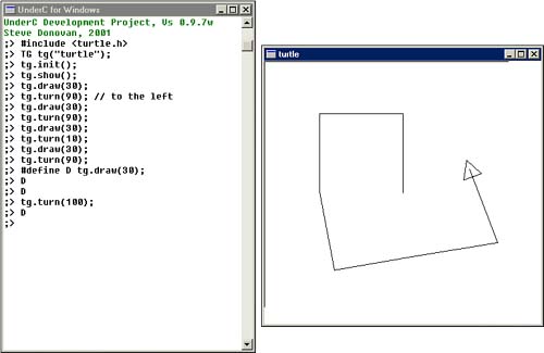
;> #include <turtle.h>
;> TG tg("turtle");
;> tg.init();
;> tg.show();
;> tg.draw(30);
;> tg.turn(90);
;> tg.draw(20);
						

In an interactive session, typing these commands can become tedious. The C++ preprocessor can help you define suitable macros to avoid some of the typing. Here is how the #define directive can save typing:

;> #define L tg.turn(+90);
;> #define R tg.turn(-90);
;> #define F tg.draw(10);
;> F
							L
							F
							R
						

A symbol that has been defined (using #define) is replaced by its definition, including the final semicolon. So, for example, L expands to tg.turn(+90);.

The state of the turtle at any point is its orientation and position. The type TG_State can be used to store this state for later. In the following example, you reset the turtle with setup() and create a variable of type TG_State:

;> tg.setup();
;> TG_State state(tg);
;> tg.draw(2);
;> state.save();
;> tg.turn(45);
;> tg.draw(2);
;> state.restore();
;> tg.turn(-45);
;> tg.draw(2);
						

In this example, you draw a line, save the state, turn right and draw, restore the state, and turn left and draw. (Type these commands to see their effects for yourself!) The result is a Y pattern. Now consider how to draw this Y using Cartesian coordinates; it's not too difficult. But if you had turned the turtle by an angle before the last set of commands, then the Y would have been at an angle. That is, any shape drawn with turtle graphics can be easily rotated by setting the initial orientation. And this is genuinely tricky to do with conventional plotting calls.

You can generate interesting patterns by using recursion. The following recursive function draws a tree:

void draw_tree(TG& tg, double l, double fact,
            double ang=45.0, double eps=0.1)
{
 TG_State state(tg);
 if (l < eps) return;
 //---- Draw the line
 tg.draw(l);
 //---- Save state, turn right, and draw the right branches
 state.save();
 tg.turn(ang);
 draw_tree(tg,fact*l,fact,ang,eps);
 //---- Restore state, turn left, and draw the left branches
 state.restore();
 tg.turn(-ang);
 draw_tree(tg,fact*l,fact,ang,eps);
}

Again, the stopping condition is the first thing you check, and this is when the length (l) passed to the function is less than some small number (eps). Note that the left and the right sides of the tree are drawn by calls to draw_tree(), but using a length of l*fact, where fact must be less than 1.0. So eventually, l will be small enough, and the recursion will end. In practice, this function can go wild if you aren't careful. If you launch this function from main() using UnderC and use #r to run the program, then #s can be used to stop the program at any point.

Note that the function saves the turtle graphics orientation and position in state, which remembers where you started. The call to draw_tree() also defines a variable, state, but (and this is the crucial bit) this is distinct from the last values. Useful recursion is possible only because automatic variables are allocated on the stack, which is why languages such as FORTRAN and BASIC traditionally couldn't handle recursion.

Figures 6.2 and 6.3 show the result of calling draw_tree() with two different angles of branching.

The power of using recursion to model biological trees comes from the nature of growth. The genes of the tree don't determine each twig; they determine the twig-sprouting recipe, and they supply local rules that generate the pattern.