IP Address Space Depletion

The growing demand for IP addresses has put a severe strain on the classful model. Most companies requesting Class B addresses have estimated that a Class B address would best accommodate their requirements because of the balance between the number of networks and the number of hosts. A Class A was overkill, with more than 16 million hosts, and a Class C had too few hosts per network. By 1991, it was becoming obvious that the Class B consumption was not slowing and actions needed to be taken to prevent its depletion.

Some of the measures consisted of creative assignment of IP addresses and promoting the use of private addresses for organizations that did not have global Internet connectivity. Other measures resulted in the initiation of working groups and directorates such as the Routing and Addressing (ROAD) working group and the IP next generation (IPng) directorate. In 1992, the ROAD working group proposed the use of classless interdomain routing (CIDR) as a measure to move away from classful IP addressing. At the same time, the IPng directorate was working on developing a new and improved IP addressing scheme that uses IP version 6 (IPv6), which would eventually solve the utilization problems that IPv4 addressing has encountered.

The measures to handle IP address depletion can be grouped into the following four categories:

• Creative IP address allocation

• Classless interdomain routing (CIDR)^[4]

• Private IP addressing and Network Address Translation (NAT)^[5], ^[7]

• IP version 6 (IPv6)^[8]

Accompanying concerns of depletion, growing IP address demand generated a need to convert the IP addressing allocation process from a central registry. Originally, the IANA and the Internet Registry (IR) had complete control of address assignment. IP addresses were assigned to organizations sequentially without consideration of geographical factors and of how or where an organization would be connecting to the Internet. This method had the effect of punching holes in the IP address space—segregating individual or small numbers of IP addresses and eliminating large, contiguous ranges of numbers.

A different approach was needed in which large, contiguous ranges of addresses are given to different administrations (such as service providers), and those service providers in turn allocate customer addresses from their own space. In general, this funnel-down method of address allocation predicts a more controlled and hierarchical method of IP address distribution. It is somewhat similar to the approach employed by the telephone network allocation scheme, where area codes are associated with regions (service provider networks), prefixes with subsets of those regions (service provider customers), and the remainder with individual customers (hosts).

IP Address Allocation

Class A network numbers are limited resources, and the allocation from this space is restricted. Although Class A space will continue to be distributed, it's now being allocated on a subnetwork basis, rather than in entire classful boundaries. Class B addresses are restricted as well, and are allocated on a subnetwork basis. Class C addresses are usually allocated from the upstream service provider's address space. Table 3-4 summarizes the current allocation of Class C address space.

Table 3-4. Class C Address Assignment Summary

Organization Requirement	Address Assignment
Fewer than 256 addresses	1 Class C network
Fewer than 512 but more than 256 addresses	2 contiguous Class C networks
Fewer than 1,024 but more than 512 addresses	4 contiguous Class C networks
Fewer than 2,048 but more than 1,024 addresses	8 contiguous Class C networks
Fewer than 4,096 but more than 2,048 addresses	16 contiguous Class C networks
Fewer than 8,192 but more than 4,096 addresses	32 contiguous Class C networks
Fewer than 16,384 but more than 8,192 addresses	64 contiguous Class C networks

Regional Internet Registries such as the American Registry for Internet Numbers (ARIN) are now hesitant to allocate space directly to end-user networks. In order to obtain address space directly from ARIN, a network must first justify allocation of at least 16 Class C addresses, or 4,096 hosts. Even with justification, administrators with requests of these sizes are encouraged to obtain address space from their providers.

Suggested user assignment guidelines, current allocation policies, request templates, and other related information can be found on ARIN's Web server (http://www.arin.net).

As far as geographic allocation of address space is concerned, there are four major areas: Europe, North America and sub-Saharan Africa, the Pacific Rim, and South and Central America. Table 3-5 summarizes allocations reserved for these regions. The multiregional area represents network numbers that were assigned prior to the implementation of this plan.

Table 3-5. Address Space Allocation among Major Geographic Areas

Address Space	Area of Allocation	Date Allocated
61.0.0.0 to 61.255.255.255	APNIC—Pacific Rim	April 1997
62.0.0.0 to 62.255.255.255	RIPE NCC—Europe	April 1997
63.0.0.0 to 63.255.255.255	ARIN	April 1997
64.0.0.0 to 64.255.255.255	ARIN	July 1999
128.0.0.0 to 191.255.255.255	Various Registries	May 1993
192.0.0.0 to 192.255.255.255	Multiregional	May 1993
193.0.0.0 to 195.255.255.255	RIPE NCC—Europe	May 1993
196.0.0.0 to 198.255.255.255	Various registries	May 1993
199.0.0.0 to 199.255.255.255	ARIN—North America	May 1993
200.0.0.0 to 200.255.255.255	ARIN—Central and South America	May 1993
201.0.0.0 to 201.255.255.255	Reserved—Central and South America	May 1993
202.0.0.0 to 203.255.255.255	APNIC—Pacific Rim	May 1993
204.0.0.0 to 205.255.255.255	ARIN—North America	March 1994
206.0.0.0 to 206.255.255.255	ARIN—North America	April 1995
207.0.0.0 to 207.255.255.255	ARIN—North America	November 1995
208.0.0.0 to 208.255.255.255	ARIN—North America	April 1996
209.0.0.0 to 209.255.255.255	ARIN—North America	June 1996
210.0.0.0 to 210.255.255.255	APNIC—Pacific Rim	June 1996
211.0.0.0 to 211.255.255.255	APNIC—Pacific Rim	June 1996
212.0.0.0 to 212.255.255.255	RIPE NCC—Europe	October 1997
213.0.0.0 to 213.255.255.255	RIPE NCC—Europe	March 1999
216.0.0.0 to 217.255.255.255	ARIN—North America	April 1998

Classless Interdomain Routing

In recent years, the global IP routing tables have grown in a way that caused routers to start becoming saturated due to processing power and memory allocation. Statistics and growth rate projections suggest that routing tables have doubled in size every 10 months between 1991 and 1995 and have grown significantly since 1998. Figure 3-9 illustrates this growth.

Without any plan of action, the routing table would have grown to about 80,000 routes in 1995. Actual data in early 2000, however, showed that the routing table size was around 76,000 routes. This reduction in growth is due to the IP address allocation scheme discussed in the previous section and to the adoption of CIDR.

CIDR was an evolutionary step beyond traditional classful IP addresses—namely, Class A, B, and C networks. In CIDR, an IP network is represented by a prefix, which is the IP address of a network, followed by a slash and, lastly, an indication of the number of leftmost contiguous bits corresponding to the network mask to be associated with that network address. For example, consider network 198.32.0.0 with a prefix of /16, written as 198.32.0.0/16. The /16 indicates that there are 16 bits of mask counting from the far left. This is synonymous to IP network 198.32.0.0 with a netmask of 255.255.0.0.

A network is referred to as a supernet when a prefix netmask boundary contains fewer bits than a network's natural mask. A Class C network 198.32.1.0, for example, has a natural mask of 255.255.255.0, which corresponds to a /24 in CIDR notation. The representation 198.32.0.0 255.255.0.0 can also be represented as 198.32.0.0/16, both of which have a shorter mask than the natural mask (16 is less than 24); hence, the network is referred to as a supernet. Figure 3-10 illustrates these address schemes.

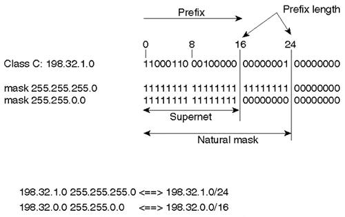
This notation provides a mechanism to easily lump all the more-specific routes of 198.32.0.0/16 (such as 198.32.0.0, 198.32.1.0, 198.32.2.0, and so on) into one advertisement referred to as an aggregate.

It is easy to be confused by all the terminology, especially because the terms aggregate, CIDR block, and supernet are often used interchangeably. Generally, these terms all indicate that a group of contiguous IP networks has been summarized into one route announcement. More precisely, CIDR is represented by the <prefix/length> notation, supernets have a prefix length shorter than the natural mask, and aggregates represent any summary route.

All the networks that are a subset of an aggregate or CIDR block are usually referred to as more specific because they provide more information about the location of a network. More specific prefixes have a longer prefix length than the aggregate:

• 198.213.0.0/16 has an aggregate of length 16

• 198.213.1.0/20 has a more-specific prefix with a length of 20

Routing domains that are CIDR-capable are referred to as classless, in contrast to the traditional classful routing domains. CIDR has depicted a new, more hierarchical Internet architecture, where each domain takes its IP address from a higher hierarchical level. This offers tremendous savings in route propagation, especially when summarization is done close to leaf or stub networks. Leaf or stub networks are end points on the global networks; they do not, in turn, provide Internet connectivity to other networks. An ISP that supports numerous leaf networks subdivides its subnets into many smaller blocks of addresses to serve those customers. Aggregation permits an ISP to advertise one IP network, generally represented as a supernet, rather than many individual advertisements, thus resulting in more efficient routing strategies and propagation, as well as introducing stability of route advertisements. Figure 3-11 illustrates the efficiency of aggregation.

In this example, ISP3 has been given the block 198.0.0.0 through 198.1.255.255 (198.0.0.0/15). ISP3 then allocates two smaller blocks of its addresses to ISP1 and ISP2. ISP1 is allocated the range 198.1.0.0 through 198.1.127.255 (198.1.0.0/17), and ISP2 is allocated the range 198.1.128.0 through 198.1.255.255 (198.1.128.0.0/17). In the same manner, ISP1 and ISP2 allocate their own customers a block of addresses from their own ranges. The left-side instance of Figure 3-11 shows what happens if CIDR is not used: ISP1 and ISP2 advertise all subnets from their customers, and ISP3 passes all these advertisements to the outside world. This results in a major increment in the global IP routing table size.

The right-side instance of Figure 3-11 portrays the same scenario when CIDR is applied. ISP1 and ISP2 perform aggregation in their customer subnets, ISP1 advertises the aggregate 198.1.0.0/17, and ISP2 advertises the aggregate 198.1.128.0/17. In the same manner, ISP3 performs aggregation on its customer subnets, ISP1 and ISP2, and sends only one aggregate (198.0.0.0/15) to its peer networks. This results in tremendous savings in the global IP routing tables.

As you can see, aggregation results in more significant efficiency gains when done close to the leaf node because the majority of the subnets to be aggregated are deployed on the customer network. Aggregation at higher levels, such as ISP3, results in a further reduction because it is dealing with fewer networks that are learned from downstream customer networks.

Aggregation works optimally if every customer connects to its provider via one connection only, which is referred to as single-homing, and also if the customer has taken its IP addresses from its provider's CIDR blocks. Unfortunately, this is not always the case in the real world. For example, situations arise where customers already have IP addresses that were not allocated from their provider's address space. As another example, some customers (who could be providers themselves) have found the need to connect to multiple providers at the same time, a scenario referred to as multihoming. These situations result in further complications and less flexibility in aggregation.

The Longest Match Routing Rule

Routing to any destination is always done on a longest match basis: A router that has to decide between two different length prefixes of the same network will always follow the longer mask. Suppose, for example, that a router has the following two entries in its routing table:

198.32.1.0/24 via path 1

198.32.0.0/16 via path 2

When attempting to deliver traffic to host 192.32.1.1, the router tries to match the destination that has the longest prefix and will deliver the traffic via Path 1 in the example. Figure 3-12 illustrates the longest match routing rule. Domain C is receiving the two updates 198.32.1.0/24 and 198.32.0.0/16, and traffic toward 198.32.1.1 is following Path 1.

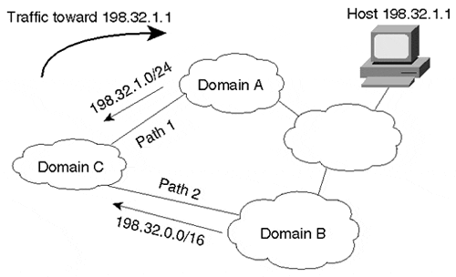
If Path 1 were to become unavailable for some reason, traffic would utilize the next closest match in the routing table, which in this case is Path 2. In cases where Domain C is receiving identical routing updates with masks of equal length coming from Domain A and Domain B, Domain C would select one path or the other, or perhaps both, depending on the load-balancing techniques offered by the specific routing implementation running in the domain.

The longest match rule implies that a destination connected to multiple domains must always be explicitly announced—that is, announced in its most specific nonaggregate form—by these domains. In Figure 3-12, because Domain B does not explicitly advertise route 198.32.1.0/24, traffic from the customer toward the host must always prefer the path via the longest prefix match, through Domain A. Such a routing configuration might place an unacceptable burden on Domain A.

Less-Specific Routes of a Network's Own Aggregate

A specific rule of routing states that, for the sake of preventing routing loops, a network must not follow a less-specific route for a destination that matches one of its own aggregated routes. A routing loop occurs when traffic circles back and forth between network elements, never reaching its final destination. Default routes 0.0.0.0/0 are a special case of this rule. A network should not follow the default route to reach destinations that are part of its aggregated advertisements. This is why routing protocols that handle aggregation of routes should always keep a bit bucket (Null0 route in Cisco parlance) to the aggregate route itself. Traffic sent to the bit bucket will be discarded, which prevents potential looping situations.

Figure 3-13 illustrates ISP1 aggregating its domain into a single route 198.32.0.0/13.

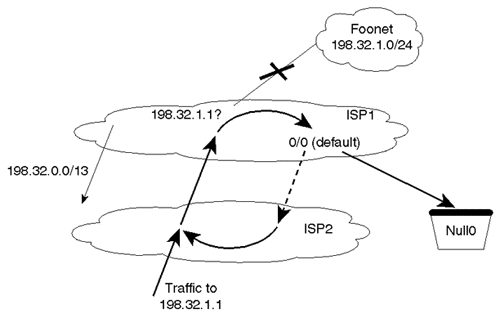
Assume that the connection between ISP1 and its customer Foonet (where network 198.32.1.0/24 exists) becomes unavailable. Suppose also that ISP1 has a default route 0.0.0.0/0 that points to ISP2 for addresses not known to ISP1. Traffic toward 198.32.1.1 following the aggregate route to ISP1 will not find the destination and will follow the default route back to ISP2. The traffic will loop back and forth between ISP1 and ISP2. To prevent such a loop, a null entry to the aggregate route, 198.32.0.0/13, is installed in ISP1's routers. The null route entry will drop all packets bound for an unreachable destination that is less specific than the aggregate route.

Aggregation, if not properly applied, can result in routing loops or black holes. A black hole occurs when traffic reaches and stops at a destination that is not its intended destination and from which it cannot be forwarded. These and other routing challenges will become more apparent as you learn about multiple address allocation schemes and how they interact with aggregation.

Single-Homing Scenario: Addresses Taken from Outside the Provider's Address Space

The routing rules discussed so far, along with the nature of a network's address space and whether it is single-homed or multihomed, have implications for whether and how the network can aggregate addresses. This section and the next three sections examine several scenarios.

In the single-homing scenario, the customer is connected to a single provider and has IP address space totally different from the provider's. This could have occurred because the customer changed providers and kept the addresses of the previous provider. Usually in this situation, customers are encouraged or forced to renumber into new address space. If renumbering does not take place, the new provider cannot aggregate the customer's addresses. Moreover, the old provider cannot aggregate as efficiently as it once did because a hole has been punched in its address space. The overall effect of using an old provider's address space is that more routes must be installed in the global Internet routing tables.

This scenario is discussed further in future chapters, but for now, network administrators should keep in mind that if their network is single-homed, the best routing option is usually the simplest one. In the single-homed case, pointing default to your provider and having the provider statically route your address space to you is usually the most trouble-free approach available. Only when multiple connections and redundancy become an issue should you consider more-complicated solutions.

The KISS (Keep It Simple, Stupid) principle, which every designer, architect, engineer, and administrator should practice, suggests that the simplest solution available is very often the best solution.

Multihoming Scenario: Addresses Taken from One Provider

In this scenario (depicted in a moment in Figure 3-14), customers are connected to multiple providers. Customers are small enough that they need to take IP addresses from only one of their multiple providers, or they were allocated the addresses while they were single-homed. We will consider two ISPs (ISP1 and ISP2) and their customers: Onenet, Twonet, and Stubnet. For each domain, Table 3-6 lists the IP address ranges, corresponding aggregates, and providers.

Table 3-6. List of Customers and Corresponding Providers

Domain	Address Range	Aggregate	Provider	Address Taken From
ISP1	198.24.0 to 198.31.255.255	198.24.0.0/13
Onenet	198.24.0.0 to 198.24.15.0	198.24.0.0/20	ISP1, ISP2	ISP1
Stubnet	198.24.16.0 to 198.24.23.0	198.24.16.0/21	ISP1	ISP1
Twonet	198.24.56.0 to 198.24.63.0	198.24.56.0/21	ISP1, ISP2	ISP1
ISP2	198.32.0.0 to 198.39.255.255	198.32.0.0/13

Note that Onenet and Twonet are multihomed to ISP1 and ISP2 with their address ranges taken from ISP1 (see Figure 3-14).

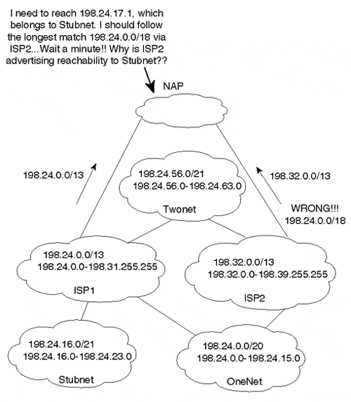
Advertising aggregates is a tricky business. Customers and ISPs have to be careful about the IP address ranges that the aggregate covers. No one is allowed to aggregate someone else's routes (proxy aggregation) unless the aggregating party is a supernet of the other party or both parties are in total agreement. In the following example, you will see how ISP2 can cause a routing black hole by aggregating the ranges coming from Onenet and Twonet.

If ISP2 were to send an aggregate that summarizes Onenet and Twonet into one update (198.24.0.0/18), as shown in Figure 3-14, a routing black hole would occur. For example, Stubnet, which is a customer of ISP1, has an IP address space that falls inside the aggregate 198.24.0.0/18. If ISP2 were to advertise the aggregate, traffic to Stubnet would follow the longest match of an IP prefix and end up blackholed in ISP2. This is why ISP2 must specifically announce each of the IP address ranges of its downstream customers that are not part of its own address space that it has in common with ISP1 (198.24.0.0/20 for Onenet and 198.24.56.0/21 for Twonet). In addition, ISP2 must announce its own address space of 198.32.0.0/13.

Figure 3-15 shows the correctly advertised aggregates. ISP2 has advertised the aggregates from Onenet and Twonet explicitly. This way, traffic destined for Stubnet will never go to ISP2.

Note in Figure 3-15 that ISP1 is also advertising explicit aggregates of Onenet and Twonet. If ISP1 were to advertise only the less-specific aggregate 198.24.0.0/13, all traffic toward Onenet and Twonet would prefer the more-specific longest match path via ISP2.

Multihoming Scenario: Addresses Taken from Different Providers

One possibility for large domains is to take IP addresses from different providers based on geographic location. Consider Figure 3-16. Largenet has taken its IP addresses from two different providers, ISP1 and ISP2. With this design, each provider will be able to aggregate its own address space without having to list specific ranges from the other provider. ISP1 would advertise the aggregate 198.24.0.0/13, and ISP2 would advertise the aggregate 198.32.0.0/13. Both aggregates are supersets of IP address blocks given to Largenet.

The major drawback with the design illustrated in Figure 3-16 is that backup routes to multihomed organizations are not maintained. ISP2 is advertising only its block of addresses and not the block taken from ISP1. In case ISP1 has problems and the 198.24.0.0/13 is lost, traffic to Largenet destined for 198.24.0.0/20 will be affected because it is not advertised anywhere else. The same reasoning applies to Largenet's addresses taken from ISP2. If the link to ISP2 fails, accessibility of the 198.32.0.0/20 range will be impaired. To remedy this situation, ISP1 has to advertise 198.32.0.0/20, and ISP2 has to advertise 198.24.0.0/20.

Multihoming Scenario: Addresses Taken from None of the Providers

Figure 3-17 illustrates a situation in which addresses are taken from a range totally different from ISP1 or ISP2's address space. In this case, both ISP1 and ISP2 advertise a specific aggregate (202.24.0.0/20) in addition to their own ranges (198.24.0.0/13 and 198.32.0.0/13). The drawback of this method is that all routers in the Internet must have a specific route to the new range introduced. Too many such instances would result in a significant increase in the global Internet routing table size.

Aggregation Recommendations

In conclusion, a domain that has been allocated a range of addresses has the sole authority (and responsibility) for aggregation of its addresses. When a domain performs aggregation, it should aggregate as much as possible without introducing ambiguity, which is possible in the case of multihomed networks.

Different situations require different designs. No single specific solution can handle all cases. It is recommended that single-homed customers obtain a single contiguous prefix from their direct provider and perform static routing to their ISP if possible, thereby avoiding potential problems with more-complicated, unnecessary configurations. If single-homed customers change providers, they should plan to transition to the new provider's address space. For multihomed customers, address assignments should be conducted in such a way that aggregation is maximized as much as possible. In the case where aggregation impacts redundancy, redundancy should prevail even if extra networks have to be listed.

The introduction of CIDR has helped dampen the explosion of global Internet routing tables tremendously over the last few years. Border Gateway Protocol version 4 (BGP-4) is the interdomain routing protocol of choice on the Internet, in part because it so efficiently handles route aggregation and propagation between domains. As this book progresses, you will see more examples of the importance of CIDR in controlling traffic behavior and stability.

For additional information on CIDR, current and historical Internet routing table sizes, and some other interesting information, follow the references provided in Appendix A.

Private Addressing and Network Address Translation

To find ways to slow down the pace at which IP addresses were being allocated, it was important to identify different connectivity requirements and to try to assign IP addresses accordingly.

Most organizations' connectivity needs fall into the following categories:

• Global connectivity

• Private connectivity

Global Connectivity

Global connectivity means that hosts inside an organization have access to both internal and Internet hosts. In this case, hosts have to be configured with globally unique IP addresses that are recognized inside and outside the organization. Organizations requiring global connectivity must request IP addresses from their service providers.

Private Connectivity

Private connectivity means that hosts inside an organization have access to internal hosts only, not Internet hosts. Examples of hosts that require only private connectivity include bank ATM machines, cash registers in a retail store, or any hosts that do not require connectivity to hosts outside the company. Private hosts need to have IP addresses that are unique inside the organization. For this type of connectivity, the IANA has reserved the following three blocks of the IP address space for what are referred to as "private internets":

• 10.0.0.0 through 10.255.255.255 (a single Class A network number)

• 172.16.0.0 through 172.31.255.255 (16 contiguous Class B network numbers)

• 192.168.0.0 through 192.168.255.255 (256 contiguous Class C network numbers)

Additional information on their use, as well as other reserved network numbers, can be found in Internet RFC 1918^[5].

An enterprise that picks its addresses from the preceding ranges does not need to get permission from IANA or an Internet Registry. Hosts that get a private IP address can connect with any other host inside the organization, but they cannot connect to hosts outside the organization without going through a proxy gateway device. The reason is that IP packets leaving the internal network will have a source IP address that is ambiguous outside the company and that cannot be reached via external networks. Because multiple companies building private networks can use the same private IP address, fewer unique global IP addresses need to be assigned.

Hosts having private addresses can coexist with hosts having global addresses. Figure 3-18 illustrates such an environment.

Companies may choose to make most of their hosts private and still keep particular segments with hosts having global addresses. The latter hosts can reach the Internet as usual. Companies that use private addresses and still have connectivity to the Internet have the responsibility of applying routing filters to prevent the private addresses from being leaked to the Internet. Most service providers, however, should apply explicit policies to incoming routing updates from customers that permit only their global IP space.

The drawback of this approach is that if an organization later decides to open its hosts to the Internet, the private IP address will have to be renumbered to use the new global IP space. With the introduction of new protocols such as the Dynamic Host Configuration Protocol (DHCP)^[6], this task has become much simpler. DHCP provides a mechanism for transmitting configuration parameters (including IP addresses) to hosts using the TCP/IP protocol suite. If the hosts are DHCP-capable, hosts can get their new addresses dynamically from a central server.

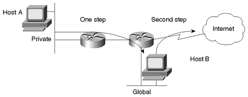
A second option is to install a bastion host that acts as a gateway between the private network and the global Internet. Host A in Figure 3-19 has a private IP address. If it wants to Telnet to a destination outside the company, it can do so by first logging in to Host B and then Telnetting from Host B to the outside. Packets leaving the company would now have Host B's source IP address, which is globally reachable. A third option is to use a Network Address Translator.

Network Address Translator

Companies migrating from a private address space to a global address space can do so with the help of Network Address Translator (NAT)^[7] technology. NAT technology lets private networks connect to the Internet without resorting to renumbering IP addresses. A NAT router is placed at the border of a domain; it translates the private addresses into global addresses, and vice versa, when internal hosts need to communicate with destinations on the Internet.

In Figure 3-20, Hosts A and B have private IP addresses 10.1.1.1 and 10.1.1.2, respectively.

If Hosts A and B want to reach a destination outside the company, the NAT device will convert the source IP addresses of the packets according to a predefined (or dynamic) mapping in the NAT table on the device. Packets from Host A will reach an outside destination as coming from source IP address 128.213.x.y. Hosts in the global domain will be unaware that the address translation is taking place, and they will reply to the global address. Packets returning from an outside host will have the destination address of the packets mapped back to the private IP address of the internal source host of the conversation.

A detailed discussion of NAT devices is beyond the scope of this book primarily because they have to handle many "corner cases" and more-involved situations. Such cases include enterprises that have used addresses that are not part of the IANA private addresses. In this case, an IR could have already assigned the address space used to some other company. Other situations involve enterprises that are assigned fewer global addresses than their number of internal hosts. In this case, the NAT must dynamically map private IP addresses to a smaller pool of global addresses.

NAT functionality doesn't always require a dedicated device, and it is often available in router software already deployed in a network. For example, Cisco Systems offers NAT as part of Cisco Internetwork Operating System (IOS).

IP Version 6

IP version 6 (IPv6)^[8], also known as IP next generation (IPng), is a move to improve the existing IPv4 implementation.

The IPng proposal was released in July 1992 at an Internet Engineering Task Force (IETF) meeting in Boston, and a number of working groups were formed in response. IPv6 tackles issues such as IP address depletion, quality of service capabilities, node auto-configuration, authentication, and security capabilities.

IPv6 is still in the experimental stage. It is not easy for companies and administrators who are deeply invested in the IPv4 architecture to migrate to a totally new architecture. As long as the IPv4 implementation keeps providing hooks and techniques (as cumbersome as they might seem) to tackle all the major issues that IPv6 is expressly designed to solve, adopting IPv6 does not seem very compelling to many companies. How soon or how late people will migrate to IPv6 is yet to be seen. This book touches on only part of the IPv6 addressing scheme and how it compares to what you have already seen with IPv4.

IPv6 addresses are 128 bits long, compared to 32 bits in IPv4. This should provide ample address space to handle address depletion and scalability issues in the Internet. 128 bits of addressing translates to 2¹²⁸, which is a large number of addresses!

The types of IPv6 addresses are indicated by the leftmost bits of the address in a variable-length field referred to as the Format Prefix (FP) (see Figure 3-21).

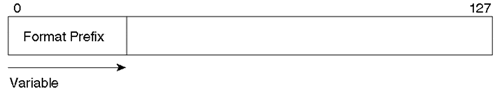
Table 3-7 outlines the initial allocation of those prefixes. IPv6 has defined multiple types of addresses. For the sake of this discussion, we are interested in the provider-based unicast addresses and the local use addresses for companies with IPv4 techniques.

Table 3-7. Allocation of IPv6 Prefixes

Description	Format Prefix
Reserved	0000 0000
Unassigned	0000 0001
Reserved for NSAP allocation	0000 001
Reserved for IPX allocation	0000 010
Unassigned	0000 011
Unassigned	0000 1
Unassigned	0001
Unassigned	001
Provider-based unicast addresses	010
Unassigned	011
Reserved for geographic unicast addresses	100
Unassigned	101
Unassigned	110
Unassigned	1110
Unassigned	1111 0
Unassigned	1111 10
Unassigned	1111 110
Unassigned	1111 1110 0
Link-local-use addresses	1111 1110 10
Site-local-use addresses	1111 1110 11
Multicast addresses	1111 1111

Provider-Based Unicast Addresses

Provider-based unicast addresses are similar to IPv4 global addresses. Figure 3-22 illustrates their format.

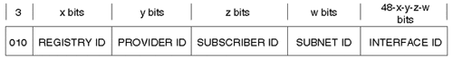
Descriptions of the fields for the provider-based unicast addresses are as follows:

• Format prefix— The first three bits are 010, indicating a provider-based unicast address.

• REGISTRY ID— Identifies the Internet address registry that assigns the PROVIDER ID.

• PROVIDER ID— Identifies the service provider responsible for the address.

• SUBSCRIBER ID— Identifies which subscriber is connected to the service provider.

• SUBNET ID— Identifies the physical link to which the address belongs.

• INTERFACE ID— Identifies a single interface among interfaces that belong to the SUBNET ID. For example, this could be the traditional 48-bit IEEE-802 Media Access Control (MAC) address.

IPv6 global addresses incorporate the CIDR functions of the IPv4 scheme. Addresses are defined in such a way as to allow hierarchy, where each entity takes its portion of the address from an entity above it (see Figure 3-23).

Local-Use Addresses

Local-use addresses are similar to the IPv4 private addresses defined in RFC 1918. Local-use addresses are divided into two types:

• Link-local-use (prefix 1111111010), which are private to a particular physical segment

• Site-local-use (prefix 1111111011), which are private to a particular site

Figure 3-24 illustrates the format of these local-use addresses.

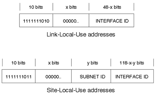
Local-use addresses have local meaning. Link-local addresses have local meaning to a particular segment, and site-local addresses have local meaning to a particular site.

Companies that are not connected to the Internet can easily assign their own addresses without a need for requesting prefixes from the global address space. If the company later decides to connect to the global Internet, a REGISTRY ID, PROVIDER ID, and SUBSCRIBER ID will be assigned with the already assigned local addresses. This is a major advantage over having to replace all private addresses with global addresses or using NAT tables to get things working in the IPv4 addressing scheme.