

Composite data types are types that are composed of other, more primitive, types. Examples of composite data types commonly found in applications include pointers, arrays, records or structures, and unions. Many high-level languages provide syntactical abstractions for these composite data types that make them easy to declare and use, all the time hiding their underlying complexities.
Though the cost of using these composite data types is not terrible, it is very easy for a programmer to introduce inefficiencies into an application by using these data types without understanding the underlying costs. Great programmers, therefore, are cognizant of the costs associated with using composite data types so they can use them in an appropriate manner. This chapter discusses the costs associated with these composite data types to better enable you to write great code.
A pointer is a variable whose value refers to some other object. Now you’ve probably experienced pointers firsthand in Pascal, C/C++, or some other programming language, and you may be feeling a little anxious right now. Well, fear not! Pointers are actually easy to deal with.
Probably the best place to start is with the definition of a pointer. High-level languages like Pascal and C/C++ hide the simplicity of pointers behind a wall of abstraction. This added complexity tends to frighten programmers because they don’t understand what’s going on behind the scenes. However, a little knowledge can erase all your fears of pointers.
Let’s just ignore pointers for a moment and work with something that’s easier to understand: an array. Consider the following array declaration in Pascal:
M: array [0..1023] of integer;
Even if you don’t know Pascal, the concept here is easy to understand. M is an array with 1,024 integers in it, indexed from M[0] to M[1023]. Each one of these array elements can hold an integer value that is independent of the others. In other words, this array gives you 1,024 different integer variables each of which you access via an array index rather than by name.
If you have a program with the statement M[0]:=100; it probably wouldn’t take you any time to figure out what this statement is doing. It stores the value 100 into the first element of the array M. Now consider the following two statements:
i := 0; (* assume i is an integer variable *)
M [i] := 100;
You should agree, without too much hesitation, that these two statements do the same thing as M[0]:=100;. Indeed, you’re probably willing to agree that you can use any integer expression in the range 0..1,023 as an index of this array. The following statements still perform the same operation as our earlier statement:
i := 5;      (* assume all variables are integers*)
j := 10;
k := 50;
m [i * j - k] := 100;
Okay, how about the following:
M [1] := 0;
M [ M [1] ] := 100;
Whoa! Now that takes a few moments to digest. However, if you take it slowly, it makes sense and you’ll discover that these two instructions perform the same operation as before. The first statement stores zero into array element M[1]. The second statement fetches the value of M[1], which is zero, and uses that value to determine where it stores the value 100.
If you’re willing to accept this example as reasonable — perhaps bizarre, but usable nonetheless — then you’ll have no problems with pointers, because M[1] is a pointer! Well, not really, but if you were to change “M” to “memory” and treat each element of this array as a separate memory location, then this is the definition of a pointer: a pointer is a memory variable whose value is the address of some other memory object.
Although most languages implement pointers using memory addresses, a pointer is actually an abstraction of a memory address, and therefore a language could define a pointer using any mechanism that maps the value of the pointer to the address of some object in memory. Some implementations of Pascal, for example, use offsets from some fixed memory address as pointer values. Some languages (such as dynamic languages like LISP) might actually implement pointers by using double indirection. That is, the pointer object contains the address of some memory variable whose value is the address of the object to be accessed. This double indirection may seem somewhat convoluted, but it does offer certain advantages when using a complex memory management system. However, this chapter will assume that a pointer is a variable whose value is the address of some other object in memory.
As you’ve seen in examples from previous chapters, you can indirectly access an object using a pointer with two 80x86 machine instructions (or with a similar sequence on other CPUs), as follows:
mov( PointerVariable, ebx );   // Load the pointer variable into a register.
mov( [ebx], eax );             // Use register indirect mode to access data.
Now consider the double-indirect pointer implementation described earlier. Access to data via double indirection is less efficient than the straight pointer implementation because it takes an extra machine instruction to fetch the data from memory. This isn’t obvious in a high-level language like C/C++ or Pascal, where you’d use double indirection as follows (it looks very similar to single indirection):
i = **cDblPtr;            // C/C++
i := ^^pDblPtr;           (* Pascal *)
In assembly language, however, you’ll see the extra work involved:
mov( hDblPtr, ebx );  // Get the pointer to a pointer.
mov( [ebx], ebx );    // Get the pointer to the value.
mov( [ebx], eax );    // Get the value.
Contrast this with the two assembly instructions (shown earlier) needed to access an object using single indirection. Because double indirection requires 50 percent more code than single indirection, you can see why many languages implement pointers using single indirection.
Pointers typically reference anonymous variables that you allocate on the heap (a region in memory reserved for dynamic storage allocation) using memory allocation/deallocation functions in different languages like malloc/free (C), new/dispose (Pascal), and new/delete (C++). Objects you allocate on the heap are known as anonymous variables because you refer to them by their address, and you do not associate a name with them. And because the allocation functions return the address of an object on the heap, you would typically store the function’s return result into a pointer variable. True, the pointer variable may have a name, but that name applies to the pointer’s data (an address), not the name of the object referenced by this address.
Most languages that provide the pointer data type let you assign addresses to pointer variables, compare pointer values for equality or inequality, and indirectly reference an object via a pointer. Some languages allow additional operations; we’re going to look at the possibilities in this section.
Many languages provide the ability to do limited arithmetic with pointers. At the very least, these languages will provide the ability to add an integer constant to a pointer, or subtract an integer constant from a pointer. To understand the purpose of these two arithmetic operations, note the syntax of the malloc function in the C standard library:
ptrVar = malloc( bytes_to_allocate );The parameter you pass malloc specifies the number of bytes of storage to allocate. A good C programmer will generally supply an expression like sizeof( int ) as the parameter to malloc. The sizeof function returns the number of bytes needed by its single parameter. Therefore, sizeof( int ) tells malloc to allocate at least enough storage for an int variable. Now consider the following call to malloc:
ptrVar = malloc( sizeof( int ) * 8 );
If the size of an integer is 4 bytes, this call to malloc will allocate storage for 32 bytes. The malloc function allocates these 32 bytes at consecutive addresses in memory (see Figure 7-1).
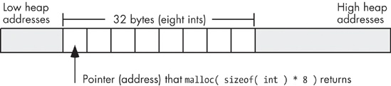
The pointer that malloc returns contains the address of the first integer in this set, so the C program will only be able to directly access the very first of these eight integers. To access the individual addresses of the other seven integers, you will need to add an integer offset to the base address. On machines that support byte-addressable memory (such as the 80x86), the address of each successive integer in memory is the address of the previous integer plus the size of an integer. For example, if a call to the C standard library malloc routine returns the memory address $0300_1000, then the eight 4-byte integers that malloc allocates will lie at the following memory addresses:
Integer | Memory Addresses |
|---|---|
0 | $0300_1000..$0300_1003 |
1 | $0300_1004..$0300_1007 |
2 | $0300_1008..$0300_100b |
3 | $0300_100c..$0300_100f |
4 | $0300_1010..$0300_1013 |
5 | $0300_1014..$0300_1017 |
6 | $0300_1018..$0300_101b |
7 | $0300_101c..$0300_101f |
Because these integers described in the preceding section are exactly four bytes apart, we need only add four to the address of the first integer to obtain the address of the second integer; likewise, the address of the third integer is the address of the second integer plus four, and so on. In assembly language, we could access these eight integers using code like the following:
malloc( @size( int32 ) * 8 );  // Returns storage for eight int32 objects.
                               // EAX points at this storage.
mov( 0, ecx );
mov( ecx, [eax] );             // Zero out the 32 bytes (four bytes
mov( ecx, [eax+4] );           //  at a time).
mov( ecx, [eax+8] );
mov( ecx, [eax+12] );
mov( ecx, [eax+16] );
mov( ecx, [eax+20] );
mov( ecx, [eax+24] );
mov( ecx, [eax+28] );
Notice the use of the 80x86 indexed addressing mode to access the eight integers that malloc allocates. The EAX register maintains the base address (first address) of the eight integers that this code allocates, and the constant appearing in the addressing mode of the mov instructions selects the offset of the specific integer from this base address.
Most CPUs use byte addresses for memory objects. Therefore, when allocating multiple copies of some n-byte object in memory, the objects will not begin at consecutive memory addresses; instead, they will appear in memory at addresses that are n bytes apart. Some machines, however, do not allow a program to access memory at an arbitrary address in memory; they require that applications access data on address boundaries that are a multiple of a word, a double word, or even a quad word. Any attempt to access memory on some other boundary will raise an exception and (possibly) halt the application. If a high-level language supports pointer arithmetic, it must take this fact into consideration and provide a generic pointer arithmetic scheme that is portable across many different CPU architectures. The most common solution that high-level languages use when adding an integer offset to a pointer is to multiply that offset by the size of the object that the pointer references. That is, if you’ve got a pointer p to a 16-byte object in memory, then p + 1 points 16 bytes beyond where p points. Likewise, p + 2 points 32 bytes beyond the address contained in the pointer p. As long as the size of the data object is a multiple of the required alignment size (which the compiler can enforce by adding padding bytes, if necessary), this scheme avoids problems on those architectures that require aligned data access.
An important thing to realize is that the addition operator only makes sense between a pointer and an integer value. For example, in the C/C++ language you can indirectly access objects in memory using an expression like *(p + i) (where p is a pointer to an object and i is an integer value). It doesn’t make any sense to add two pointers together. Similarly, it isn’t reasonable to add other data types with a pointer. For example, adding a floating-point value to a pointer makes no sense. What would it mean to reference the data at some base address plus 1.5612? Operations on pointers involving strings, characters, and other data types don’t make much sense, either. Integers (signed and unsigned) are the only reasonable values to add to a pointer.
On the other hand, not only can you add an integer to a pointer, you can also add a pointer to an integer and the result is still pointer (both p + i and i + p are legal). This is because addition is commutative.
Another reasonable pointer arithmetic operation is subtraction. Subtracting an integer from a pointer references a memory location immediately before the address held in the pointer. However, subtraction is not commutative and subtracting a pointer from an integer is not a legal operation (p − i is legal, but i − p is not).
In C/C++ *(p × i) accesses the ith object immediately before the object at which p points. In 80x86 assembly language, as in assembly on many processors, you can also specify a negative constant offset when using an indexed addressing mode, e.g.,
mov( [ebx−4], eax );
Keep in mind, that 80x86 assembly language uses byte offsets, not object offsets (as C/C++ does). Therefore, this statement loads into EAX the double word in memory immediately preceding the memory address in EBX.
Unlike addition, it actually makes sense to subtract the value of one pointer variable from another. Consider the following C/C++ code that marches through a string of characters looking for the first e character that follows the first a that it finds:
int distance;
char *aPtr;
char *ePtr;
. . .
aPtr = someString; // Get ptr to start of string in aPtr.
// While we're not at the end of the string and the current
// char isn't 'a':
while( *aPtr != '�' && *aPtr != 'a' )
{
aPtr = aPtr + 1; // Move on to the next character pointed
// at by aPtr.
}
// While we're not at the end of the string and the current
// character isn't 'e':
ePtr = aPtr; // Start at the 'a' char (or end of string
// if no 'a').
while( *ePtr != '�' && *ePtr != 'a' )
{
ePtr = ePtr + 1; // Move on to the next character pointed at by aPtr.
}
// Now compute the number of characters between the 'a' and the 'e'
// (counting the 'a' but not counting the 'e'):
distance = (ePtr - aPtr);The subtraction of these two pointers produces the number of data objects that exist between the two pointers (in this case, ePtr and aPtr point at characters, so the subtraction result produces the number of characters, or bytes, between the two pointers).
The subtraction of two pointer values only makes sense if the two pointers reference the same data structure in memory (for example, pointing at characters within the same string, as in this C/C++ example). Although C/C++ (and certainly assembly language) will allow you to subtract two pointers that point at completely different objects in memory, their difference will probably have very little meaning.
When using pointer subtraction in C/C++, the base types of the two pointers must be identical (that is, the two pointers must contain the addresses of two objects whose types are identical). This restriction exists because pointer subtraction in C/C++ produces the number of objects between the two pointers, not the number of bytes. It wouldn’t make any sense to compute the number of objects between a byte in memory and a double word in memory; would you be counting the number of bytes or the number of double words in this case? Of course, in assembly language you can get away with this (and the result is always the number of bytes between the two pointers), but it still doesn’t make much sense semantically.
Note that the subtraction of two pointers could return a negative number if the left pointer operand is at a lower memory address than the right pointer operand. Depending on your language and its implementation, you may need to take the absolute value of the result if you’re only interested in the distance between the two pointers and you don’t care which pointer contains the greater address.
Comparisons are another set of operations that make sense for pointers. Almost every language that supports pointers will let you compare two pointers to see if they are equal or not equal. Such a comparison will tell you whether the pointers reference the same object in memory. Some languages (such as assembly and C/C++) will also let you compare two pointers to see if one pointer is less than or greater than another. This only makes sense, however, if the pointers have the same base type and both pointers contain the address of some object within the same data structure (such as an array, string, or record). If the comparison of two pointers suggests that the value of one pointer is less than the other, then this tells you that the first pointer references an object within the data structure appearing before the object referenced by the second pointer. The converse is equally true for the greater than comparison.
After strings, arrays are probably the most common composite data type (a complex data type built up from smaller data objects). Yet few beginning programmers fully understand how arrays operate and know about their efficiency trade-offs. It’s surprising how many novice programmers view arrays from a completely different perspective once they understand how arrays operate at the machine level.
Abstractly, an array is an aggregate data type whose members (elements) are all of the same type. A member is selected from the array by specifying the member’s array index with an integer (or with some value whose underlying representation is an integer, such as character, enumerated, and Boolean types). This chapter assumes that all of the integer indexes of an array are numerically contiguous (though this is not required). That is, if both x and y are valid indexes of the array, and if x < y, then all i such that x < i < y are also valid indexes. In this book, we will assume that array elements occupy contiguous locations in memory. An array with five elements will appear in memory as shown in Figure 7-2.
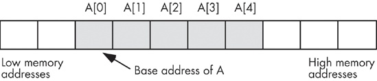
The base address of an array is the address of the first element of the array and is at the lowest memory location. The second array element directly follows the first in memory, the third element follows the second, and so on. Note that there is no requirement that the indexes start at zero. They may start with any number as long as they are contiguous. However, for the purposes of this discussion, it’s easier to discuss array access if the first index is zero. We’ll generally begin most arrays at index zero unless there is a good reason to do otherwise.
Whenever you apply the indexing operator to an array, the result is the unique array element specified by that index. For example, A[i] chooses the ith element from array A.
Array declarations are very similar across many high-level languages. We’ll look at some examples in many of these languages within this section.
C, C++, and Java all let you declare an array by specifying the total number of elements in an array. The syntax for an array declaration in these languages is as follows:
data_type array_name[number_of_elements];
Here are some sample C/C++ array declarations:
char CharArray[ 128 ];
int intArray[ 8 ];
unsigned char ByteArray[ 10 ];
int *PtrArray[ 4 ];
If these arrays are declared as automatic variables, then C/C++ “initializes” them with whatever bit patterns happen to be present in memory. If, on the other hand, you declare these arrays as static objects, then C/C++ zeros out each array element. If you want to initialize an array yourself, then you can use the following C/C++ syntax:
data_type array_name[number_of_elements] = {element_list};
Here’s a typical example:
int intArray[8] = {0,1,2,3,4,5,6,7};HLA’s array declaration syntax takes the following form, which is semantically equivalent to the C/C++ declaration:
array_name:data_type[number_of_elements];
Here are some examples of HLA array declarations, which all allocate storage for uninitialized arrays (the second example assumes that you have defined the integer data type in a type section of the HLA program):
static

    CharArray: char[128];         // Character array with elements
                                  //  0..127.
    IntArray: integer[ 8 ];       // Integer array with elements 0..7.
    ByteArray: byte[10];          // Byte array with elements 0..9.
    PtrArray: dword[4];           // Double-word array with elements 0..3.
You can also initialize the array elements using declarations like the following:
RealArray: real32[8] := [ 0.0, 1.0, 2.0, 3.0, 4.0, 5.0, 6.0, 7.0 ];
IntegerAry: integer[8] := [ 8, 9, 10, 11, 12, 13, 14, 15 ];
Both of these definitions create arrays with eight elements. The first definition initializes each 4-byte real32 array element with one of the values in the range 0.0..7.0. The second declaration initializes each integer array element with one of the values in the range 8..15.
Pascal/Delphi/Kylix uses the following syntax to declare an array:
array_name: array[lower_bound..upper_bound] ofdata_type;
As in the previous examples, array_name is the identifier and data_type is the type of each element in this array. Unlike C/C++, Java, and HLA, in Pascal/Delphi/Kylix you specify the upper and lower bounds of the array rather than the array’s size. The following are typical array declarations in Pascal:
type
        ptrToChar = ^char;
var
        CharArray: array[0..127] of char;           // 128 elements
        IntArray: array[ 0..7 ] of integer;         // 8 elements
        ByteArray: array[0..9] of char;             // 10 elements
        PtrArray: array[0..3] of ptrToChar;         // 4 elements
Although these Pascal examples start their indexes at zero, Pascal does not require a starting index of zero. The following is a perfectly valid array declaration in Pascal:
var
        ProfitsByYear : array[ 1998..2009 ] of real;  // 12 elements
The program that declares this array would use indexes 1998 through 2009 when accessing elements of this array, not 0 through 11.
Many Pascal compilers provide an extra feature to help you locate defects in your programs. Whenever you access an element of an array, these compilers will automatically insert code that will verify that the array index is within the bounds specified by the declaration. This extra code will stop the program if the index is out of range. For example, if an index into ProfitsByYear is outside the range 1998..2009, the program would abort with an error. This is a very useful feature that helps verify the correctness of your program.[30]
Generally, array indexes are integer values, though some languages allow other ordinal types (those data types that use an underlying integer representation). For example, Pascal allows char and boolean array indexes. In Pascal, it’s perfectly reasonable and useful to declare an array as follows:
alphaCnt : array[ 'A'..'Z' ] of integer;
You access elements of alphaCnt using a character expression as the array index. For example, consider the following Pascal code that initializes each element of alphaCnt to zero:
for ch := 'A' to 'Z' do
    alphaCnt[ ch ] := 0;
Assembly language and C/C++ treat most ordinal values as special instances of integer values, so they are certainly legal array indexes. Most implementations of BASIC will allow a floating-point number as an array index, though BASIC always truncates the value to an integer before using it as an index.[31]
Abstractly, an array is a collection of variables that you access using an index. Semantically, we can define an array any way we please as long as it maps distinct indexes to distinct objects in memory and always maps the same index to the same object. In practice, however, most languages utilize a few common algorithms that provide efficient access to the array data.
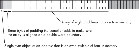
The number of bytes of storage an array will consume is the product of the number of elements multiplied by the number of bytes per element in the array. Many languages also add a few additional bytes of padding at the end of the array so that the total length of the array is an even multiple of a nice value like four (on a 32-bit machine, a compiler may add bytes to the end of the array in order to extend its length to some multiple of four bytes). However, a program must not access these extra padding bytes because they may or may not be present. Some compilers will put them in, some will not, and some will only put them in depending on the type of object that immediately follows the array in memory.
Many optimizing compilers will attempt to place an array starting at a memory address that is an even multiple of some common size like two, four, or eight bytes. This effectively adds padding bytes before the beginning of the array or, if you prefer to think of it this way, it adds padding bytes to the end of the previous object in memory (see Figure 7-3).
On those machines that do not support byte-addressable memory, those compilers that attempt to place the first element of an array on an easily accessed boundary will allocate storage for an array on whatever boundary the machine supports. If the size of each array element is less than the minimum size memory object the CPU supports, the compiler implementer has two options:
Allocate the smallest accessible memory object for each element of the array
Pack multiple array elements into a single memory cell
The first option has the advantage of being fast, but it wastes memory because each array element carries along some extra storage that it doesn’t need. The second option is compact, but it requires extra instructions to pack and unpack data when accessing array elements, which means that accessing elements is slower. Compilers on such machines often provide an option that lets you specify whether you want the data packed or unpacked so you can make the choice between space and speed.
If you’re working on a byte-addressable machine (like the 80x86) then you probably don’t have to worry about this issue. However, if you’re using a high-level language and your code might wind up running on a different machine at some point in the future, you should choose an array organization that is efficient on all machines.
If you allocate all the storage for an array in contiguous memory locations, and the first index of the array is zero, then accessing an element of a one-dimensional array is simple. You can compute the address of any given element of an array using the following formula:
Element_Address = Base_Address + index * Element_Size
The Element_Size item is the number of bytes that each array element occupies. Thus, if the array contains elements of type byte, the Element_Size field is one and the computation is very simple. If each element of the array is a word (or another two-byte type) then Element_Size is two. And so on.
Consider the following Pascal array declaration:
var SixteenInts : array[ 0..15] of integer;
To access an element of the SixteenInts on a byte-addressable machine, assuming 4-byte integers, you’d use this calculation:
Element_Address = AddressOf( SixteenInts) + index*4
In assembly language (where you would actually have to do this calculation manually rather than having the compiler do the work for you), you’d use code like the following to access array element SixteenInts[index]:
mov( index, ebx );
mov( SixteenInts[ ebx*4 ], eax );
Most CPUs can easily handle one-dimensional arrays. Unfortunately, there is no magic addressing mode that lets you easily access elements of multi-dimensional arrays. That’s going to take some work and several machine instructions.
Before discussing how to declare or access multidimensional arrays, it would be a good idea to look at how to implement them in memory. The first problem is to figure out how to store a multidimensional object in a one-dimensional memory space.
Consider for a moment a Pascal array of the following form:
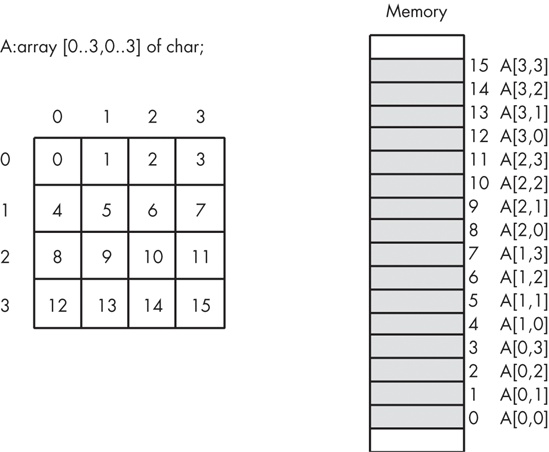
A:array[0..3,0..3] of char;
This array contains 16 bytes organized as four rows of four characters. Somehow you have to draw a correspondence between each of the 16 bytes in this array and each of the 16 contiguous bytes in main memory. Figure 7-4 shows one way to do this.
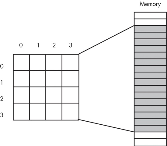
The actual mapping is not important as long as two things occur:
No two entries in the array occupy the same memory location(s)
Each element in the array always maps to the same memory location
Therefore, what you really need is a function with two input parameters — one for a row and one for a column value — that produces an offset into a contiguous block of 16 memory locations.
Any old function that satisfies these two constraints will work fine. However, what you really want is a mapping function that is efficient to compute at run time and that works for arrays with any number of dimensions and any bounds on those dimensions. While there are a large number of possible functions that fit this bill, there are two functions that most high-level languages use: row-major ordering and column-major ordering.
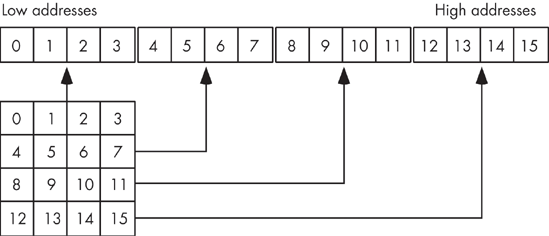
Row-major ordering assigns array elements to successive memory locations by moving across the rows and then down the columns. Figure 7-5 demonstrates this mapping.
Row-major ordering is the method employed by most high-level programming languages including Pascal, C/C++, Java, Ada, and Modula-2. It is very easy to implement and is easy to use in machine language. The conversion from a two-dimensional structure to a linear sequence is very intuitive. Figure 7-6 on the next page provides another view of the ordering of a 4×4 array.
The actual function that converts the set of multidimensional array indexes into a single offset is a slight modification of the formula for computing the address of an element of a one-dimensional array. The formula to compute the offset for a 4×4 two-dimensional row-major ordered array given an access of this form:
A[ colindex][ rowindex ]
. . . is as follows:
Element_Address = Base_Address + (colindex * row_size + rowindex) * Element_Size
As usual, Base_Address is the address of the first element of the array (A[0][0] in this case) and Element_Size is the size of an individual element of the array, in bytes. Row_size is the number of elements in one row of the array (four, in this case, because each row has four elements). Assuming Element_Size is one, this formula computes the following offsets from the base address:
For a three-dimensional array, the formula to compute the offset into memory is only slightly more complex. Consider a C/C++ array declaration given as follows:
someType A[depth_size][col_size][row_size];If you have an array access similar to A[depth_index][col_index][row_index] then the computation that yields the offset into memory is the following:
Address =
Base + ((depth_index * col_size + col_index)*row_size + row_index) * Element_Size

Element_size is the size, in bytes, of a single array element.
For a four-dimensional array, declared in C/C++ as:
type A[bounds0][bounds1][bounds2][bounds3];. . . the formula for computing the address of an array element when accessing element A[i][j][k][m] is as follows:
Address =
    Base + (((i * bounds1 + j) * bounds2 + k) * bounds3 + m) * Element_Size
If you’ve got an n-dimensional array declared in C/C++ as follows:
dataType A[bn-1][bn-2]...[b0];. . . and you wish to access the following element of this array:
A[an-1][an-2]...[a1][a0]
. . . then you can compute the address of a particular array element using the following algorithm:
Address := an-1
for i := n-2 downto 0 do
    Address := Address * bi + ai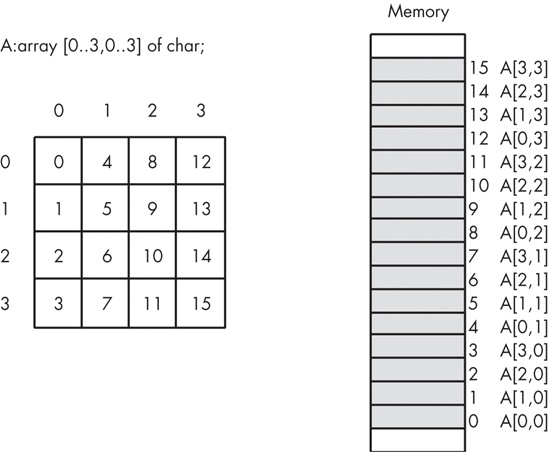
Address := Base_Address + Address*Element_SizeColumn-major ordering is the other common array element address function. FORTRAN and various dialects of BASIC (such as older versions of Microsoft BASIC) use this scheme to index arrays. Pictorially, a column-major ordered array is organized as shown in Figure 7-7.
The formula for computing the address of an array element when using column-major ordering is very similar to that for row-major ordering. The difference is that you reverse the order of the index and size variables in the computation. That is, rather than working from the leftmost index to the rightmost, you operate on the indexes from the rightmost towards the leftmost.
For a two-dimensional column-major array, the formula is as follows:
Element_Address =
    Base_Address + (rowindex * col_size + colindex) * Element_Size
The formula for a three-dimensional column-major array is the following:
Element_Address =
    Base_Address +
        ((rowindex*col_size+colindex) * depth_size + depthindex) * Element_Size
And so on. Other than using these new formulas, accessing elements of an array using column-major ordering is identical to accessing arrays using row-major ordering.
If you have an m × n array, it will have m × n elements and will require m × n × Element_Size bytes of storage. To allocate storage for an array you must reserve this amount of memory. With one-dimensional arrays, the syntax that the different high-level languages employ is very similar. However, their syntax starts to diverge when you consider multidimensional arrays.
In C, C++, and Java, you use the following syntax to declare a multi-dimensional array:
data_type array_name [dim1][dim2] . . . [dimn];Here is a concrete example of a three-dimensional array declaration in C/C++:
int threeDInts[ 4 ][ 2 ][ 8 ];
This example creates an array with 64 elements organized with a depth of four by two rows by eight columns. Assuming each int object requires 4 bytes, this array consumes 256 bytes of storage.
Pascal’s syntax actually supports two equivalent ways of declaring multi-dimensional arrays. The following example demonstrates both of these forms:
var
        threeDInts  : array[0..3] of array[0..1] of array[0..7] of integer;
        threeDInts2 : array[0..3, 0..1, 0..7] of integer;
Semantically, there are only two major differences that exist among different languages. The first difference is whether the array declaration specifies the overall size of each array dimension or whether it specifies the upper and lower bounds. The second difference is whether the starting index is zero, one, or a user-specified value.
Accessing an element of a multidimensional array in a high-level language is so easy that a typical programmer will do so without considering the associated cost. In this section, we’ll look at some of the assembly language sequences you’ll need to access elements of a multidimension array to give you a clearer picture of these costs.
Consider again, the C/C++ declaration of the ThreeDInts array from the previous section:
int ThreeDInts[ 4 ][ 2 ][ 8 ];
In C/C++, if you wanted to set element [i][j][k] of this array to the value of n, you’d probably use a statement similar to the following:
ThreeDInts[i][j][k] = n;
This statement, however, hides a great deal of complexity. Recall the formula needed to access an element of a three-dimensional array:
Element_Address =
    Base_Address +
        ((rowindex * col_size + colindex) * depth_size + depthindex) *
            Element_Size
The ThreeDInts example does not avoid this calculation, it only hides it from you. The machine code that the C/C++ compiler generates is similar to the following:
intmul( 2, i, ebx );    // EBX = 2 * i
add( j, ebx );          // EBX = 2 * i + j
intmul( 8, ebx );       // EBX = (2 * i + j) * 8
add( k, ebx );          // EBX = (2 * i + j) * 8 + k
mov( n, eax );
mov( eax, ThreeDInts[ebx*4] );  // ThreeDInts[i][j][k] = n
Actually, ThreeDInts is special. The sizes of all the array dimensions are nice powers of two. This means that the CPU can use shifts instead of multiplication instructions to multiply EBX by two and by four in this example. Because shifts are often faster than multiplication, a decent C/C++ compiler will generate the following code:
mov( i, ebx );
shl( 1, ebx );          // EBX = 2 * i
add( j, ebx );          // EBX = 2 * i + j
shl( 3, ebx );          // EBX = (2 * i + j) * 8
add( k, ebx );          // EBX = (2 * i + j) * 8 + k
mov( n, eax );
mov( eax, ThreeDInts[ebx*4] );  // ThreeDInts[i][j][k] = n
Note that a compiler can only use this faster code if an array dimension is a power of two. This is the reason many programmers attempt to declare arrays whose dimension sizes are some power of two. Of course, if you must declare extra elements in the array to achieve this goal, you may wind up wasting space (especially with higher-dimensional arrays) to achieve a small increase in speed.
For example, if you need a 10×10 array and you’re using row-major ordering, you could create a 10×16 array to allow the use of a shift (by four) instruction rather than a multiply (by 10) instruction. When using column-major ordering, you’d probably want to declare a 16×10 array to achieve the same effect, since row-major calculation doesn’t use the size of the first dimension when calculating an offset into an array, and column-major calculation doesn't use the size of the second dimension when calculating an offset. In either case, however, the array would wind up having 160 elements instead of 100 elements. Only you can decide if this extra space is worth the small increase in speed you’ll gain.
Another major composite data structure is the Pascal record or C/C++ structure. The Pascal terminology is probably better, as it avoids confusion with the term data structure. Therefore, we’ll adopt the term record here.
An array is homogeneous, meaning that its elements are all of the same type. A record, on the other hand, is heterogeneous and its elements can have differing types. The purpose of a record is to let you encapsulate logically related values into a single object.
Arrays let you select a particular element via an integer index. With records, you must select an element, known as a field, by the field’s name. Each of the field names within the record must be unique. That is, the same field name may not appear two or more times in the same record. However, all field names are local to their record, and you may reuse those names elsewhere in the program.
Here’s a typical record declaration for a Student data type in Pascal/Delphi:
type
        Student =
                record
                        Name:     string [64];
                        Major:    smallint;    // 2-byte integer in Delphi
                        SSN:      string[11];
                        Mid1:     smallint;
                        Midt:     smallint;
                        Final:    smallint;
                        Homework: smallint;
                        Projects: smallint;
                end;
Many Pascal compilers allocate all of the fields in contiguous memory locations. This means that Pascal will reserve the first 65 bytes for the name,[32] the next 2 bytes hold the major code, the next 12 bytes the Social Security number, and so on.
Here’s the same declaration in C/C++:
typedef
        struct
        {
                char Name[65]; // Room for a 64-character zero-terminated string.
                short Major;   // Typically a 2-byte integer in C/C++
                char SSN[12];  // Room for an 11-character zero-terminated string.
                short Mid1;
                short Mid2;
                short Final;
                short Homework;
                short Projects
} Student;In HLA, you can also create structure types using the record/endrecord declaration. In HLA, you would encode the record from the previous sections as follows:
type
    Student:
        record
            Name:     char[65];    // Room for a 64-character
                                   //  zero-terminated string.
            Major:    int16;
            SSN:      char[12];    // Room for an 11-character
                                   //  zero-terminated string.
            Mid1:     int16;
            Mid2:     int16;
            Final:    int16;
            Homework: int16;
            Projects: int16;
        endrecord;
As you can see, the HLA declaration is very similar to the Pascal declaration. Note that to stay consistent with the Pascal declaration, this example uses character arrays rather than strings for the Name and SSN (Social Security number) fields. In a typical HLA record declaration, you’d probably use a string type for at least the Name field (keeping in mind that a string variable is a four-byte pointer).
The following Pascal example demonstrates a typical Student variable declaration:
var
        John: Student;
Given the earlier declaration for the Pascal Student data type, this allocates 81 bytes of storage laid out in memory as shown in Figure 7-8.
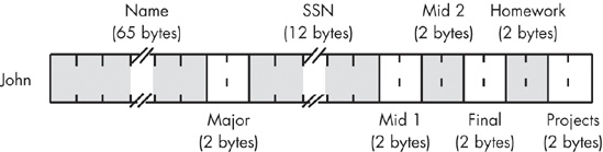
If the label John corresponds to the base address of this record, then the Name field is at offset John + 0, the Major field is at offset John + 65, the SSN field is at offset John + 67, and so on.
Most programming languages let you refer to a record field by its name rather than by its numeric offset into the record. The typical syntax for field access uses the dot operator to select a field from a record variable. Given the variable John from the previous example, here’s how you could access various fields in this record:
John.Mid1 = 80;              // C/C++ example
John.Final := 93;            (* Pascal Example *)
mov( 75, John.Projects );    // HLA example
Figure 7-8 suggests that all fields of a record appear in memory in the order of their declaration. In theory, a compiler can freely place the fields anywhere in memory that it chooses. In practice, though, almost every compiler places the fields in memory in the same order they appear within the record declaration. The first field usually appears at the lowest address in the record, the second field appears at the next highest address, the third field follows the second field in memory, and so on.
Figure 7-8 also suggests that compilers pack the fields into adjacent memory locations with no gaps between the fields. While this is true for many languages, this certainly isn’t the most common memory organization for a record. For performance reasons, most compilers will actually align the fields of a record on appropriate memory boundaries. The exact details vary by language, compiler implementation, and CPU, but a typical compiler will place fields at an offset within the record’s storage area that is “natural” for that particular field’s data type. On the 80x86, for example, compilers that follow the Intel ABI (application binary interface) will allocate one-byte objects at any offset within the record, words only at even offsets, and double-word or larger objects on double-word boundaries. Although not all 80x86 compilers support the Intel ABI, most do, which allows records to be shared among functions and procedures written in different languages on the 80x86. Other CPU manufacturers provide their own ABI for their processors and programs that adhere to an ABI can share binary data at run time with other programs that adhere to the same ABI.
In addition to aligning the fields of a record at reasonable offset boundaries, most compilers will also ensure that the length of the entire record is a multiple of two, four, or eight bytes. They accomplish this by adding padding bytes at the end of the record to fill out the record’s size. The reason that compilers pad the size of a record is to ensure that the record’s length is an even multiple of the size of the largest scalar (non-composite data type) object in the record or the CPU’s optimal alignment size, whichever is smaller. For example, if a record has fields whose lengths are one, two, four, eight, and ten bytes long, then an 80x86 compiler will generally pad the record’s length so that it is an even multiple of eight. This allows you to create an array of records and be assured that each record in the array starts at a reasonable address in memory.
Although some CPUs don’t allow access to objects in memory at misaligned addresses, many compilers allow you to disable the automatic alignment of fields within a record. Generally, the compiler will have an option you can use to globally disable this feature. Many of these compilers also provide a pragma or a packed keyword of some sort that lets you turn off field alignment on a record-by-record basis. Disabling the automatic field alignment feature may allow you to save some memory by eliminating the padding bytes between the fields (and at the end of the record), provided that field misalignment is acceptable on your CPU. The cost, of course, is that the program may run a little bit slower when it needs to access misaligned values in memory.
One reason to use a packed record is to gain manual control over the alignment of the fields within the record. For example, suppose you have a couple of functions written in two different languages and both of these functions need to access some data in a record. Further, suppose that the two compilers for these functions do not use the same field alignment algorithm. A record declaration like the following (in Pascal) may not be compatible with the way both functions access the record data:
type
    aRecord: record
        bField : byte;  (* assume Pascal compiler supports a byte type *)
        wField : word;  (* assume Pascal compiler supports a word type *)
        dField : dword; (* assume Pascal compiler supports a double-word type *)
    end; (* record *)
The problem here is that the first compiler could use the offsets zero, two, and four for the bField, wField, and dField fields, respectively, while the second compiler might use offsets zero, four, and eight.
Suppose however, that the first compiler allows you to specify the packed keyword before the record keyword, causing the compiler to store each field immediately following the previous one. Although using the packed keyword will not make the records compatible with both functions, it will allow you to manually add padding fields to the record declaration, as follows:
type
    aRecord: packed record
        bField   :byte;
        padding0 :array[0..2] of byte;  (* add padding to dword align wField *)
        wField   :word;
        padding1 :word;                 (* add padding to dword align dField *)
        dField   :dword;
    end; (* record *)
Maintaining code where you’ve handled the padding in a manual fashion can be a real chore. However, if incompatible compilers need to share data, this is a trick worth knowing because it can make data sharing possible. For the exact details concerning packed records, you’ll have to consult your language’s reference manual.
A discriminant union (or just union) is very similar to a record. Like records, unions have fields and you access those fields using dot notation. In fact, in many languages, about the only syntactical difference between records and unions is the use of the keyword union rather than record. Semantically, however, there is a big difference between a record and a union. In a record, each field has its own offset from the base address of the record, and the fields do not overlap. In a union, however, all fields have the same offset, zero, and all the fields of the union overlap. As a result, the size of a record is the sum of the sizes of all the fields (plus, possibly, some padding bytes), whereas a union’s size is the size of its largest field (plus, possibly, some padding bytes at the end).
Because the fields of a union overlap, you might think that a union has little use in a real-world program. After all, if the fields all overlap, then changing the value of one field changes the values of all the other fields as well. This generally means that the use of a union’s field is mutually exclusive — that is, you can only use one field at any given time. This observation is generally correct, but although this means that unions aren’t as generally applicable as records, they still have many uses.
Here’s an example of a union declaration in C/C++:
typedef union
{
        unsigned int  i;
        float         r;
        unsigned char c[4];

} unionType;
Assuming the C/C++ compiler in use allocates four bytes for unsigned integers, the size of a unionType object will be four bytes (because all three fields are 4-byte objects).
Pascal/Delphi/Kylix use case variant records to create a discriminant union. The syntax for a case variant record is the following:
type
    typeName =
        record
            <<non-variant/union record fields go here>>

            case tag of
                const1:( field_declaration );
                const2:( field_declaration );
                    .
                    .
                    .
                constn:( field_declaration )  (* no semicolon follows
                                                 the last field *)

        end;
In this example, tag is either a type identifier (such as Boolean, char, or some user-defined type) or it can be a field declaration of the form identifier:type. If the tag item takes this latter form, then identifier becomes another field of the record (and not a member of the variant section — those declarations following the case) and has the specified type. When using this second form, the Pascal compiler could generate code that raises an exception whenever the application attempts to access any of the variant fields except the one specified by the value of the tag field. In practice, though, almost no Pascal compilers do this. Still, keep in mind that the Pascal language standard suggests that compilers should do this, so some compilers out there might actually do this check.
Here’s an example of two different case variant record declarations in Pascal:
type
        noTagRecord=
                record
                        someField: integer;
                        case boolean of
                                 true:( i:integer );
                                 false:( b:array[0..3] of char)
                end; (* record *)

        hasTagRecord=
                record
                        case which:(0..2) of
                                 0:( i:integer );
                                 1:( r:real );
                                 2:( c:array[0..3] of char )
                end; (* record *)
As you can see in the hasTagRecord union, a Pascal case-variant record does not require any normal record fields. This is true even if you do not have a tag field.
HLA supports unions as well. Here’s a typical union declaration in HLA:
type
        unionType:
                union
                        i: int32;
                        r: real32;
                        c: char[4];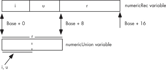
endunion;The big difference between a union and a record is the fact that records allocate storage for each field at different offsets, whereas unions overlay each of the fields at the same offset in memory. For example, consider the following HLA record and union declarations:
type
        numericRec:
                record
                        i: int32;
                        u: uns32;
                        r: real64;
                endrecord;
        numericUnion:
                union
                        i: int32;
                        u: uns32;
                        r: real64;
                endunion;
If you declare a variable, n, of type numericRec, you access the fields as n.i, n.u, and n.r, exactly as though you had declared the n variable to be type numericUnion. However, the size of a numericRec object is 16 bytes because the record contains two double-word fields and a quad-word (real64) field. The size of a numericUnion variable, however, is eight bytes. Figure 7-9 shows the memory arrangement of the i, u, and r fields in both the record and union.
In addition to conserving memory, programmers often use unions to create aliases in their code. As you may recall, an alias is a second name for some memory object. Although aliases are often a source of confusion in a program, and should be used sparingly, using an alias can sometimes be convenient. For example, in some section of your program you might need to constantly use type coercion to refer to a particular object. One way to avoid this is to use a union variable with each field representing one of the different types you want to use for the object. As an example, consider the following HLA code fragment:
type
     CharOrUns:
         union
             c:char;
             u:uns32;
         endunion;

static
    v:CharOrUns;
With a declaration like this one, you can manipulate an uns32 object by accessing v.u. If, at some point, you need to treat the LO byte of this uns32 variable as a character, you can do so by simply accessing the v.c variable, as follows:
mov( eax, v.u );
stdout.put( "v, as a character, is '", v.c, "'" nl );
Another common practice is to use unions to disassemble a larger object into its constituent bytes. Consider the following C/C++ code fragment:
typedef union
{
    unsigned int u;
    unsigned char bytes[4];
} asBytes;

asBytes composite;
         .
         .
         .
    composite.u = 1234576890;
    printf
    (
        "HO byte of composite.u is %u, LO byte is %u
",
        composite.u[3],
        composite.u[0]
    );
Although composing and decomposing data types using unions is a useful trick every now and then, be aware that this code is not portable. Remember, the HO and LO bytes of a multibyte object appear at different addresses on big endian versus little endian machines. This code fragment works fine on little endian machines, but fails to display the right bytes on big endian CPUs. Any time you use unions to decompose larger objects, you should be aware that the code might not be portable across different machines. Still, disassembling larger values into the corresponding bytes, or assembling a larger value from bytes, is usually much more efficient than using shift lefts, shift rights, and AND operations. Therefore, you’ll see this trick used quite a bit.
This chapter has dealt with the low-level implementation of common data structures you’ll find in various languages. For more information on data types, you can head off in two directions at this point — lower or higher.
To learn more about the low-level implementation of various data types, you’ll probably want to start learning and mastering assembly language. My book The Art of Assembly Language (No Starch Press) is a good place to begin that journey.
Higher-level data-structure information is available in just about any decent college textbook on data structures and algorithm design. There are literally hundreds of these books available covering a wide range of subjects.
For those interested in a combination of low-level and high-level concepts, a good choice is Donald Knuth’s The Art of Computer Programming, Volume I: Fundamental Algorithms. This text is available in nearly every book-store that carries technical books.
[30] Many Pascal compilers provide an option to turn off this array index range checking once your program is fully tested. Turning off the bounds checking improves the efficiency of the resulting program.
[31] BASIC allows you to use floating-point values as array indexes because the original BASIC language did not provide support for integer expressions; it only provided real values and string values.
[32] Pascal strings usually require an extra byte, in addition to all the characters in the string, to encode the length.