The first thing to learn about the I/O subsystem is that I/O in a typical computer system is radically different from I/O in a typical high-level programming language. At the primitive I/O levels of a computer system, you will rarely find machine instructions that behave like Pascal’s writeln, C++’s cout, C’s printf, or even like the HLA stdin and stdout statements. In fact, most I/O machine instructions behave exactly like the 80x86’s mov instruction. To send data to an output device, the CPU simply moves that data to a special memory location, and to read data from an input device, the CPU moves data from the device’s address into the CPU. I/O operations behave much like memory read and write operations, except that there are usually more wait states associated with I/O operations.

We can classify I/O ports into five categories based on the CPU’s ability to read and write data at a given port address. These five categories of ports are read-only, write-only, read/write, dual I/O, and bidirectional.

A read-only port is obviously an input port. If the CPU can only read the data from the port, then the data must come from some source external to the computer system. The hardware typically ignores any attempt to write data to a read-only port, but it’s never a good idea to write to a read-only port because some devices may fail if you do so. A good example of a read-only port is the status port on a PC’s parallel printer interface. Data from this port specifies the current status of the printer, while the hardware ignores any data written to this port.

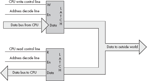
A write-only port is always an output port. Writing data to such a port presents the data for use by an external device. Attempting to read data from a write-only port generally returns whatever garbage value happens to be on the data bus. You generally cannot depend on the meaning of any value read from a write-only port. An output port typically uses a latch device to hold data to be sent to the outside world. When a CPU writes to a port address associated with an output latch, the latch stores the data and makes it available on an external set of signal lines (see Figure 12-1).

Figure 12-1. A typical output port

A perfect example of an output port is a parallel printer port. The CPU typically writes an ASCII character to a byte-wide output port that connects to the DB-25F connector on the back of the computer’s case. A cable transmits this data to the printer, where it arrives on the printer’s input port (from the printer’s perspective, it is reading the data from the computer system). A processor inside the printer typically converts this ASCII character to a sequence of dots that it prints on the paper.

Note that output ports can be write-only or read/write. The port in Figure 12-1, for example, is a write-only port. Because the outputs on the latch do not loop back to the CPU’s data bus, the CPU cannot read the data the latch contains. Both the address decode line (En) and the write control line (W) must be active for the latch to operate. If the CPU tries to read the data located at the latch’s address the address decode line is active but the write control line is not, so the latch does not respond to the read request.

A read/write port is an output port as far as the outside world is concerned. However, the CPU can read as well as write data to such a port. Whenever the CPU reads data from a read/write port, it reads the data that was last written to the port allowing a programmer to retrieve that value. The act of reading data from the port does not affect the data presented to the external peripheral device.^[46]

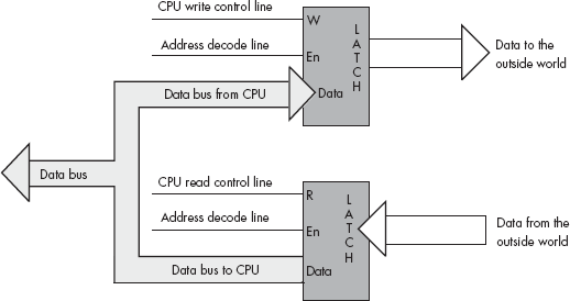
Figure 12-2 shows how to create a port that you can both read from and write to. The data written to the output port loops back to a second latch. Placing the address of these two latches on the address bus asserts the address decode lines on both latches. Therefore, to select between the two latches, the CPU must also assert either the read line or the write line. Asserting the read line (as will happen during a read operation) will enable the lower latch. This places the data previously written to the output port on the CPU’s data bus, allowing the CPU to read that data.

Figure 12-2. An output port that supports read/write access

Note that the port in Figure 12-2 is not an input port — true input ports read data from external pins. Although the CPU can read data from this latch, the organization of this circuit simply allows the CPU to read the data it previously wrote to the port, thus saving the program from maintaining this value in a separate variable if the application needs to know what was written to the port. The data appearing on the external connector is output only, and one cannot connect realworld input devices to these signal pins.

A dual I/O port is also a read/write port, but when you read a dual I/O port, you read data from an external input device rather than the last data written to the output side of the port’s address. Writing data to a dual I/O port transmits data to some external output device, just as writing to a write-only port does. Figure 12-3 shows how you could interface a dual I/O port with the system.

Figure 12-3. An input port and output device that share the same address (a dual I/O port)

Note that a dual I/O port is actually created using two ports — a read-only port and a write-only port — that share the same port address. Reading from the address accesses the read-only port, and writing to the address accesses the write-only port. Essentially, this port arrangement uses the read and write (R/W) control lines to provide an extra address bit that specifies which of the two ports to use.

A bidirectional port allows the CPU to both read and write data to an external device. To function properly, a bidirectional port must pass various control lines, such as read and write enable, to the peripheral device so that the device can change the direction of data transfer based on the CPU’s read/write request. In effect, a bidirectional port is an extension of the CPU’s bus through a bidirectional latch or buffer.

Generally, a given peripheral device will utilize multiple I/O ports. The original PC parallel printer interface, for example, uses three port addresses: a read/write I/O port, a read-only input port, and a write-only output port. The read/write port is the data port on which the CPU can read the last ASCII character written through that port. The input port returns control signals from the printer, which indicate whether the printer is ready to accept another character, is offline, is out of paper, and so on. The output port transmits control information to the printer. Later model PCs substituted a bidirectional port for the data port, allowing data transfer from and to a device through the parallel port. The bidirectional data port improved performance for various devices such as disk and tape drives connected to the PC’s parallel port.

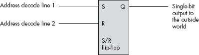
The examples given thus far may leave you with the impression that the CPU always reads and writes peripheral data using the data bus. However, while the CPU generally transfers the data it has read from input ports across the data bus, it does not always use the data bus when writing data to output ports. In fact, a very common output method is to simply access a port’s address directly without writing any data to it. Figure 12-4 illustrates a very simple example of this technique using a set/reset (S/R) flip-flop. In this circuit, an address decoder decodes two separate addresses. Any read or write access to the first address sets the output line high; any read or write access to the second address clears the output line. This circuit ignores the data on the CPU’s data lines, and it also ignores the status of the read and write lines. The only thing that matters is that the CPU accesses one of these two addresses.

Figure 12-4. Outputting data to a port by simply accessing that port

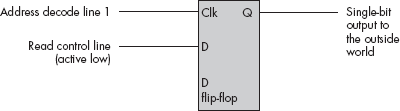
Another possible way to connect an output port to a system is to connect the read/write status lines to the data input of a D flip-flop. Figure 12-5 shows how you could design such a device. In this diagram, any read of the port sets the output bit to zero, while any write to this port sets the output bit to one.

Figure 12-5. Outputting data using the read/write control as the data to output

These examples of connecting peripheral devices directly to the CPU are only two of an amazing number of different designs that engineers have devised to avoid using the data bus. However, unless otherwise noted, the remaining examples in this chapter presume that the CPU reads and writes data to an external device using the data bus.

There are three basic I/O mechanisms that computer systems can use to communicate with peripheral devices: memory-mapped input/output, I/O-mapped input/output, and direct memory access (DMA). Memory-mapped I/O uses ordinary locations within the CPU’s memory address space to communicate with peripheral devices. I/O-mapped input/output uses an address space separate from memory, and it uses special machine instructions to transfer data between that special I/O address space and the outside world. DMA is a special form of memory-mapped I/O where the peripheral device reads and writes data located in memory without CPU intervention. Each I/O mechanism has its own set of advantages and disadvantages, which we will discuss in the following sections.

How a device connects to a computer system is usually determined by the hardware system engineer at design time, and programmers have little control over this choice. While some devices may present two different interfaces to the system, software engineers generally have to live with whatever interface the hardware designers provide. Nevertheless, by paying attention to the costs and benefits of the I/O mechanism used for communication between the CPU and the peripheral device, you can choose different code sequences that will maximize the performance of I/O within your applications.

Different peripheral devices have different data transfer rates. Some devices, like keyboards, are extremely slow when compared to CPU speeds. Other devices, like disk drives, can actually transfer data faster than the CPU can process it. The appropriate programming technique for data transfer depends strongly on the transfer speed of the peripheral device involved in the I/O operation. Therefore, in order to understand how to write the most appropriate code, it first makes sense to invent some terminology to describe the different transfer rates of peripheral devices.

The speed of the peripheral device will determine the type of I/O mechanism used for the I/O operation. Clearly, high-speed devices must use DMA because programmed I/O is too slow. Medium- and low-speed devices may use any of the three I/O mechanisms for data transfer (though low-speed devices rarely use DMA because of the cost of the extra hardware involved).

With typical bus architectures, personal computer systems are capable of one transfer per microsecond or better. Therefore, high-speed devices are those that transfer data more rapidly than once per microsecond. Medium-speed transfers are those that involve a data transfer every 1 to 100 micro-seconds. Low-speed devices usually transfer data less often than once every 100 microseconds. Of course, these definitions for the speed of low-, medium-, and high-speed devices are system dependent. Faster CPUs with faster buses allow faster medium-speed operations.

Note that one transfer per microsecond is not the same thing as a 1-MB-per-second transfer rate. A peripheral device can actually transfer more than one byte per data transfer operation. For example, when using the 80x86 in( dx, eax ); instruction, the peripheral device can transfer four bytes in one transfer. Therefore, if the device is reaching one transfer per micro-second, the device can transfer 4 MB per second using this instruction.

Earlier in this book, you saw that the CPU communicates with memory and I/O devices using the system bus. If you’ve ever opened up a computer and looked inside or read the specifications for a system, you’ve probably seen terms like PCI, ISA, EISA, or even NuBus mentioned when discussing the computer’s system bus. In this section, we’ll discuss the relationship between the CPU’s bus and these different system buses, and describe how these different computer system buses affect the performance of a system.

Although the choice of the hardware bus is made by hardware engineers, not software engineers, many computer systems will actually employ multiple buses in the same system. Therefore, software engineers can choose which peripheral devices they use based upon the bus connections of those peripherals. Furthermore, maximizing performance for a particular bus may require different programming techniques than for other buses. Finally, although a software engineer may not be able to choose the buses available in a particular computer system, that engineer can choose which system to write their software for, based on the buses available in the system they ultimately choose.

Computer system buses like PCI (Peripheral Component Interconnect) and ISA (Industry Standard Architecture) are definitions for physical connectors inside a computer system. These definitions describe the set of signals, physical dimensions (i.e., connector layouts and distances from one another), and a data transfer protocol for connecting different electronic devices. These buses are related to the CPU’s local bus, which consists of the address, data, and control lines, because many of the signals on the peripheral buses are identical to signals that appear on the CPU’s bus.

However, peripheral buses do not necessarily mirror the CPU’s bus — they often contain several lines that are not present on the CPU’s bus. These additional lines let peripheral devices communicate with one another without having to go through the CPU or memory. For example, most peripheral buses provide a common set of interrupt control signals that let I/O devices communicate directly with the system’s interrupt controller, which is also a peripheral device. Nor do the peripheral buses include all the signals found on the CPU’s bus. For example, the ISA bus only supports 24 address lines compared with the Pentium IV’s 36 address lines.

Different peripheral devices are designed to use different peripheral buses. Figure 12-6 shows the organization of the PCI and ISA buses in a typical computer system.

Figure 12-6. Connection of the PCI and ISA buses in a typical PC

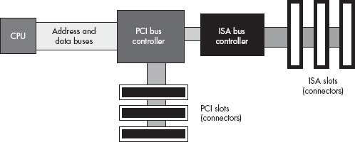
Notice how the CPU’s address and data buses connect to a PCI bus controller peripheral device, but not to the PCI bus itself. The PCI bus controller contains two sets of pins, providing a bridge between the CPU’s local bus and the PCI bus. The signal lines on the local bus are not connected directly to the corresponding lines on the PCI bus; instead, the PCI bus controller acts as an intermediary, rerouting all data transfer requests between the CPU and the PCI bus.

Another interesting thing to note is that the ISA bus controller is not directly connected to the CPU. Instead, it is usually connected to the PCI bus controller. There is no logical reason why the ISA controller couldn’t be connected directly to the CPU’s local bus. However, in most modern PCs, the ISA and PCI controllers appear on the same chip, and the manufacturer of this chip has chosen to interface the ISA bus through the PCI controller for cost or performance reasons.

The CPU’s local bus usually runs at some submultiple of the CPU’s frequency. Typical local bus frequencies are currently 66 MHz, 100 MHz, 133 MHz, 400 MHz, 533 MHz, and 800 MHz, but they may become even faster. Usually, only memory and a few selected peripherals like the PCI bus controller sit on the CPU’s bus and operate at this high frequency.

Because a typical CPU’s bus is 64 bits wide and because it is theoretically possible to achieve one data transfer per clock cycle, the CPU’s bus has a maximum possible data transfer rate of eight bytes times the clock frequency, or 800 MB per second for a 100-MHz bus. In practice, CPUs rarely achieve the maximum data transfer rate, but they do achieve some percentage of it, so the faster the bus, the more data can move in and out of the CPU (and caches) in a given amount of time.

12.5.3 The AGP Bus

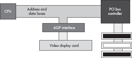
Video display cards are very special peripherals that need maximum bus performance to ensure quick screen updates and fast graphic operations. Unfortunately, if the CPU has to constantly negotiate with other peripherals for the use of the PCI bus, graphics performance can suffer. To overcome this problem, video card designers created the AGP (Accelerated Graphics Port) interface between the CPU’s local bus and the video display card, which provides various control lines and bus protocols specifically designed for video display cards.

The AGP connection lets the CPU quickly move data to and from the video display RAM (see Figure 12-7). Because there is only one AGP port per system, only one card can use the AGP slot at a time. The upside of this is that the system never has to negotiate for access to the AGP bus.

Figure 12-7. The AGP bus interface

If a particular I/O device produces or consumes data faster than the system is capable of transferring data to or from that device, the system designer has two choices: provide a faster connection between the CPU and the device, or slow down the rate of transfer between the two.

If the peripheral device is connected to a slow bus like ISA, a faster connection can be created by using a different, faster bus. Another way to increase the connection speed is by switching to a wider bus like the 64-bit PCI bus, a bus with a higher frequency, or a higher performance bus like PCI-X. System designers can also sometimes create a faster interface to the bus as they have done with the AGP connection. However, once you exhaust these possibilities for improving performance, it can be very expensive to create a faster connection between peripherals and the system.

The other alternative available when a peripheral device is capable of transferring data faster than the system is capable of processing it, is to slow down the transfer rate between the peripheral and the computer system. This isn’t always as bad an option as it might seem. Most high-speed devices don’t transfer data at a constant rate to the system. Instead, devices typically transfer a block of data rapidly and then sit idle for some length of time. Although the burst rate is high and is faster than what the CPU or memory can handle, the average data transfer rate is usually lower than this. If you could average out the high-bandwidth peaks and transfer some of the data when the peripheral was inactive, you could easily move data between the peripheral and the computer system without resorting to an expensive, high-bandwidth bus or connection.

The trick is to use memory on the peripheral side to buffer the data. The peripheral can rapidly fill this buffer with data during an input operation, and it can rapidly extract data from the buffer during an output operation. Once the peripheral device is inactive, the system can proceed at a sustainable rate either to empty or refill the buffer, depending on whether the buffer is full or empty at the time. As long as the average data transfer rate of the peripheral device is below the maximum bandwidth the system supports, and the buffer is large enough to hold bursts of data going to and from the peripheral, this scheme lets the peripheral communicate with the system at a lower average data transfer rate.

Often, to save costs, the buffering takes place in the CPU’s address space rather than in memory local to the peripheral device. In this case, it is often the software engineer’s responsibility to initialize the buffer for a peripheral device. Therefore, this buffering isn’t always transparent to the software engineer. In some cases, neither the peripheral device nor the OS provide a buffer for the peripheral’s data and it becomes the application’s responsibility to buffer up this data in order to maintain maximum performance and avoid loss of data. In other cases, the device or OS may provide a small buffer, but the application itself might not process the data often enough to avoid data overruns — in such situations, an application can create a larger buffer that is local to the application to avoid the data overruns.

Many I/O devices cannot accept data at just any rate. For example, a Pentium-based PC is capable of sending several hundred million characters per second to a printer, but printers are incapable of printing that many characters each second. Likewise, an input device such as a keyboard will never transmit several million keystrokes per second to the system (because it operates at human speeds, not computer speeds). Because of the difference in capabilities between the CPU and many of the system peripherals, the CPU needs some mechanism to coordinate data transfer between the computer system and its peripheral devices.

One common way to coordinate data transfers is to send and receive status bits on a port separate from the data port. For example, a single bit sent by a printer could tell the system whether it is ready to accept more data. Likewise, a single status bit in a different port could specify whether a keystroke is available at the keyboard data port. The CPU can test these bits prior to writing a character to the printer, or reading a key from the keyboard.

Using status bits to indicate that a device is ready to accept or transmit data is known as handshaking. It gets this name because the protocol is similar to two people agreeing on some method of transfer by a handshake.

To demonstrate how handshaking works, consider the following short 80x86 assembly language program segment. This code fragment will continuously loop while the HO bit of the printer status register (at input port $379) contains zero and will exit once the HO bit is set (indicating that the printer is ready to accept data):

mov( $379, dx );      // Initialize DX with the address of the status port.
repeat

    in( dx, al );     // Get the parallel port status into the AL register.
    and( $80, al );   // Clear Z flag if the HO bit is set.

until( @nz );         // Repeat until the HO bit contains a one.

// Okay to write another byte to the printer data port here.

One problem with the repeat..until loop in the previous section is that it could spin indefinitely as it waits for the printer to become ready to accept additional input. If someone turns the printer off, or if the printer cable becomes disconnected, the program could freeze up, forever waiting for the printer to become available. Usually, it’s a better idea to inform the user when something goes wrong rather than allowing the system to hang. Typically, great programmers handle this problem by including a time-out period in the loop, which once exceeded causes the program to alert the user that something is wrong with the peripheral device.

You can expect some sort of response from most peripheral devices within a reasonable amount of time. For example, even in the worst case, most printers will be ready to accept additional character data within a few seconds of the last transmission. Therefore, something is probably wrong if 30 seconds or more have passed without the printer accepting a new character. If the program is written to detect this kind of problem, it can pause, asking the user to check the printer and tell the program to resume printing once the problem is resolved.

Choosing a good time-out period is not an easy task. In doing so, you must carefully balance the irritation of possibly having the program incorrectly claim that something is wrong, with the pain of having the program lock up for long periods when there actually is something wrong. Both situations are equally annoying to the end user.

An easy way to create a time-out period is to count the number of times the program loops while waiting for a handshake signal from a peripheral. Consider the following modification to the repeat..until loop of the previous section:

mov( $379, dx );          // Initialize DX with the address of the status port.
mov( 30_000_000, ecx );   // Time-out period of approximately 30 seconds,
                          //  assuming port access time is about 1 microsecond.
HandshakeLoop:

    in( dx, al );         // Get the parallel port status into the AL register.
    and( $80, al );       // Clear Z flag if the HO bit is set.

loopz HandshakeLoop;      // Decrement ECX and loop while ECX <> 0 and
                          //  the HO bit of AL contains a zero.

if( ecx <> 0 ) then

    // Okay to write another byte to the printer data port here.

else

    // We had a time-out condition if we get here.

endif;

This code will exit once the printer is ready to accept data or when approximately 30 seconds have expired. You might question the 30-second figure, after all, a software-based loop (counting down ECX to zero) should run at different speeds on different processors. However, don’t miss the fact that there is an in instruction inside this loop. The in instruction reads a port on the ISA bus and that means this instruction will take approximately one microsecond to execute (about the fastest operation on the ISA bus). Hence, one million times through the loop will take about a second (plus or minus 50 percent, but close enough for our purposes). This is true almost regardless of the CPU frequency.

Polling is the process of constantly testing a port to see if data is available. The handshaking loops of the previous sections provide good examples of polling — the CPU waits in a short loop, testing the printer port’s status value until the printer is ready to accept more data, and then the CPU can transfer more data to the printer. Polled I/O is inherently inefficient. If the printer in this example takes ten seconds to accept another byte of data, the CPU spins doing nothing productive for those ten seconds.

In early personal computer systems, this is exactly how a program would behave. When a program wanted to read a key from the keyboard, it would poll the keyboard status port until a key was available. These early computers could not do other processing while waiting for the keyboard.

The solution to this problem is to use what is called an interrupt mechanism. An interrupt is triggered by an external hardware event, such as the printer becoming ready to accept another character, that causes the CPU to interrupt its current instruction sequence and call a special interrupt service routine (ISR). Typically, an interrupt service routine runs through the following sequence of events:

In most computer systems, typical I/O devices generate an interrupt whenever they make data available to the CPU, or when they become able to accept data from the CPU. The ISR quickly processes the interrupt request in the background, allowing some other computation to proceed normally in the foreground.

Though interrupt service routines are usually written by OS designers or peripheral device manufacturers, most OSes provide the ability to pass an interrupt to an application via signals or some similar mechanism. This allows you to include interrupt service routines directly within an application. You could use this facility, for example, to have a peripheral device notify your application when its internal buffer is full and the application needs to copy data from the peripheral’s buffer to an application buffer to prevent data loss.

If you’re working on Windows 95 or 98, you can write assembly code to access I/O ports directly. The assembly code shown earlier as an example of hand-shaking is a good example of this. However, recent versions of Windows and all versions of Linux employ a protected mode of operation. In this mode, direct access to devices is restricted to the OS and certain privileged programs. Standard applications, even those written in assembly language, are not so privileged. If you write a simple program that attempts to send data to an I/O port, the system will generate an illegal access exception and halt your program.

Linux does not allow just any program to access I/O ports as it pleases. Only programs with “super-user” (root) privileges may do so. For limited I/O access, it is possible to use the Linux ioperm system call to make certain I/O ports accessible from user applications. For more details, Linux users should read the “man” page on “ioperm.”

This chapter has so far introduced I/O in a very general sense, without spending too much time discussing the particular peripheral devices present in a typical PC. It some respects, it’s dangerous to discuss real devices on modern PCs because the traditional (“legacy”) devices that are easy to understand are slowly disappearing from PC designs. As manufacturers introduce new PCs, they are removing many of the legacy peripherals like parallel and serial ports that are easy to program, and they are replacing these devices with complex peripherals like USB and FireWire. Although a detailed discussion on programming these newer peripheral devices is beyond the scope of this book, you need to understand their behavior in order to write great code that accesses these devices.

Because of the nature of the peripheral devices appearing in the rest of this chapter, the information presented applies only to IBM-compatible PCs. There simply isn’t enough space in this book to cover how particular I/O devices behave on different systems. Other systems support similar I/O devices, but their hardware interfaces may be different from what’s presented here. Nevertheless, the general principles still apply.

The PC’s keyboard is a computer system in its own right. Buried inside the keyboard’s case is an 8042 microcontroller chip that constantly scans the switches on the keyboard to see if any keys are held down. This processing occurs in parallel with the normal activities of the PC, and even though the PC’s 80x86 is busy with other things, the keyboard never misses a keystroke.

A typical keystroke starts with the user pressing a key on the keyboard. This closes an electrical contact in a switch, which the keyboard’s micro-controller can sense. Unfortunately, mechanical switches do not always close perfectly clean. Often, the contacts bounce off one another several times before coming to rest with a solid connection. To a microcontroller chip that is reading the switch constantly, these bouncing contacts will look like a very quick series of keypresses and releases. If the microcontroller registers these as multiple keystrokes, a phenomenon known as keybounce may result, a problem common to many cheap and old keyboards. Even on the most expensive and newest keyboards, keybounce can be a problem if you look at the switch a million times a second, because mechanical switches simply cannot settle down that quickly. A typical inexpensive key will settle down within five milliseconds, so if the keyboard scanning software polls the key less often than this, the controller will effectively miss the keybounce. The practice of limiting how often one scans the keyboard in order to eliminate keybounce is known as debouncing.

The keyboard controller must not generate a new key code sequence every time it scans the keyboard and finds a key held down. The user may hold a key down for many tens or hundreds of milliseconds before releasing it, and we don’t want this to register as multiple keystrokes. Instead, the keyboard controller should generate a single key code value when the key goes from the up position to the down position (a down key operation). In addition to this, modern keyboards provide an autorepeat capability that engages once the user has held down a key for a given time period (usually about half a second), and it treats the held key as a sequence of keystrokes as long as the user continues to hold the key down. However, even these autorepeat keystrokes are regulated to allow only about ten keystrokes per second rather than the number of times per second the keyboard controller scans all the switches on the keyboard.

Upon detecting a down keystroke, the microcontroller sends a keyboard scan code to the PC. The scan code is not related to the ASCII code for that key; it is an arbitrary value IBM chose when the PC’s keyboard was first developed. The PC keyboard actually generates two scan codes for every key you press. It generates a down code when you press a key down and an up code when you release the key. Should you hold the key down long enough for the autorepeat operation to begin, the keyboard controller will send a sequence of down codes until you release the key, at which time the keyboard controller will send a single up code.

The 8042 microcontroller chip transmits these scan codes to the PC, where they are processed by an interrupt service routine for the keyboard. Having separate up and down codes is important because certain keys (like shift, ctrl, and alt) are only meaningful when held down. By generating up codes for all the keys, the keyboard ensures that the keyboard ISR knows which keys are pressed while the user is holding down one of these modifier keys. Exactly what the system does with these scan codes depends on the OS, but usually the OS’s keyboard device driver will translate the scan code sequence into an appropriate ASCII code or some other notation that applications can work with.

The original IBM PC design provided support for three parallel printer ports that IBM designated LPT1:, LPT2:, and LPT3:. With laser and ink jet printers still a few years in the future, IBM probably envisioned machines that could support a standard dot matrix printer, a daisy wheel printer, and maybe some other auxiliary type of printer for different purposes. Surely, IBM did not anticipate the general use that parallel ports have received or they would probably have designed them differently. Today, the PC’s parallel port controls keyboards, disk drives, tape drives, SCSI adapters, Ethernet (and other network) adapters, joystick adapters, auxiliary keypad devices, other miscellaneous devices, and, oh yes, printers.

The current trend is to eliminate the parallel port from systems because of connector size and performance problems. Nevertheless, the parallel port remains an interesting device. It’s one of the few interfaces that hobbyists can use to connect the PC to simple devices they’ve built themselves. Therefore, learning to program the parallel port is a task many hardware enthusiasts take upon themselves.

In a unidirectional parallel communication system, there are two distinguished sites: the transmitting site and the receiving site. The transmitting site places its data on the data lines and informs the receiving site that data is available; the receiving site then reads the data lines and informs the transmitting site that it has taken the data. Note how the two sites synchronize their access to the data lines — the receiving site does not read the data lines until the transmitting site tells it to, and the transmitting site does not place a new value on the data lines until the receiving site removes the data and tells the transmitting site that it has the data. In other words, this form of parallel communications between the printer and computer system relies on hand-shaking to coordinate the data transfer.

The PC’s parallel port implements handshaking using three control signals in addition to the eight data lines. The transmitting site uses the strobe (or data strobe) line to tell the receiving site that data is available. The receiving site uses the acknowledge line to tell the transmitting site that it has taken the data. A third handshaking line, busy, tells the transmitting site that the receiving site is busy and that the transmitting site should not attempt to send data. The busy signal differs from the acknowledge signal, insofar as acknowledge tells the system that the receiving site has accepted the data just sent and processed it. The busy line tells the system that the receiving site cannot accept any new data just yet; the busy line does not imply that the last character sent has been processed (or even that a character was sent).

From the perspective of the transmitting site, a typical data transmission session looks something like the following:

From the perspective of the receiving site, a typical data transmission session looks something like the following:

By carefully following these steps, the receiving and transmitting sites coordinate their actions so that the transmitting site doesn’t attempt to put several bytes on the data lines before the receiving site consumes them, and so the receiving site doesn’t attempt to read data that the transmitting site has not sent.

The RS-232 serial communication standard is probably the most popular serial communication scheme in the world. Although it suffers from many drawbacks, speed being the primary one, its use is widespread, and there are thousands of devices you can connect to a PC using an RS-232 serial interface. Though the use of the serial port is rapidly being eclipsed by USB use, many devices still use the RS-232 standard.

The original PC system design supports concurrent use of up to four RS-232 compatible devices connected through the COM1:, COM2:, COM3:, and COM4: ports. For those who need to connect additional serial devices, you can buy interface cards that let you add 16 or more serial ports to the PC.

In the early days of the PC, DOS programmers had to directly access the 8250 Serial Communications Chip (SCC) to implement RS-232 communications in their applications. A typical serial communications program would have a serial port ISR that read incoming data from the SCC and wrote outgoing data to the chip, as well as code to initialize the chip and to buffer incoming and outgoing data. Though the serial chip is very simple compared to modern peripheral interfaces, the 8250 is sufficiently complex that many programmers would have difficulty getting their serial communications software working properly. Furthermore, because serial communications was rarely the main purpose of the application being written, few programmers added anything beyond the basic serial communications features needed for their applications.

Fortunately, today’s application programmers rarely program the SCC directly. Instead, OSes such as Windows or Linux provide sophisticated serial communications device drivers that application programmers can call. These drivers provide a consistent feature set that all applications can use, and this reduces the learning curve needed to provide serial communication functionality. Another advantage to the OS device driver approach is that it removes the dependency on the 8250 SCC. Applications that use an OS device driver will automatically work with different serial communication chips. In contrast, an application that programs the 8250 directly will not work on a system that uses a USB to RS-232 converter cable. However, if the manufacturer of that USB to RS-232 converter cable provides an appropriate device driver for an OS, applications that do serial communications via that OS will automatically work with the USB/serial device.

An in-depth examination of RS-232 serial communications is beyond the scope of this book. For more information on this topic, consult your OS programmer’s guide or pick up one of the many excellent texts devoted specifically to this subject.

Almost all modern computer systems include some sort of disk drive unit to provide online mass storage. At one time, certain workstation vendors produced diskless workstations, but the relentless drop in price and increasing storage space of fixed (aka “hard”) disk units has all but obliterated the diskless computer system. Disk drives are so ubiquitous in modern systems that most people take them for granted. However, for a programmer to take a disk drive for granted is a dangerous thing. Software constantly interacts with the disk drive as a medium for application file storage, so a good understanding of how disk drives operate is very important if you want to write efficient code.

12.15.2 Hard Drives

The fixed disk drive, more commonly known as the hard disk, is without question the most common mass storage device in use today. The modern hard drive is truly an engineering marvel. Between 1982 and 2004, the capacity of a single drive unit has increased over 50,000-fold, from 5 MB to over 250 GB. At the same time, the minimum price for a new unit has dropped from $2,500 (U.S.) to below $50. No other component in the computer system has enjoyed such a radical increase in capacity and performance along with a comparable drop in price. (Semiconductor RAM probably comes in second, and paying the 1982 price today would get you about 4,000 times the capacity.)

While hard drives were decreasing in price and increasing in capacity, they were also becoming faster. In the early 1980s, a hard drive subsystem was doing well to transfer 1 MB per second between the drive and the CPU’s memory; modern hard drives transfer more than 50 MB per second. While this increase in performance isn’t as great as the increase in performance of memory or CPUs, keep in mind that disk drives are mechanical units on which the laws of physics place greater limitations. In some cases, the dropping costs of hard drives has allowed system designers to improve their performance by using disk arrays (see 12.15.3 RAID Systems, for details). By using certain hard disk subsystems like disk arrays, it is possible to achieve 320-MB-per-second transfer rates, though it’s not especially cheap to do so.

“Hard” drives are so named because their data is stored on a small, rigid disk that is usually made out of aluminum or glass and is coated with a magnetic material. The name “hard” differentiates these disks from floppy disks, which store their information on a thin piece of flexible Mylar plastic.

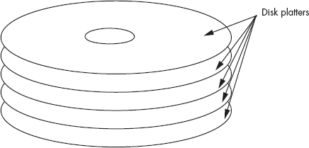
In disk drive terminology, the small aluminum or glass disk is known as a platter. Each platter has two surfaces, front and back (or top and bottom), and both sides contain the magnetic coating. During operation, the hard drive unit spins this platter at a particular speed, which these days is usually 3,600; 5,400; 7,200; 10,000; or 15,000 revolutions per minute (RPM). Generally, though not always, the faster you spin the platter, the faster you can read data from the disk and the higher the data transfer rate between the disk and the system. The smaller disk drives that find their way into laptop computers typically spin at much slower speeds, like 2,000 or 4,000 RPM, to conserve battery life and generate less heat.

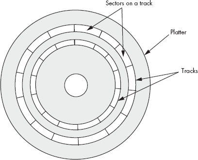
A hard disk subsystem contains two main active components: the disk platter(s) and the read/write head. The read/write head, when held stationary, floats above concentric circles, or tracks, on the disk surface (see Figure 12-8). Each track is broken up into a sequence of sections known as sectors or blocks. The actual number of sectors varies by drive design, but a typical hard drive might have between 32 and 128 sectors per track (again, see Figure 12-8). Each sector typically holds between 256 and 4,096 bytes of data, and many disk drive units let the OS choose between several different sector sizes, the most common choices being 512 bytes and 4,096 bytes.

Figure 12-8. Tracks and sectors on a hard disk platter

The disk drive records data when the read/write head sends a series of electrical pulses to the platter, which translates those electrical pulses into magnetic pulses that the platter’s magnetic surface retains. The frequency at which the disk controller can record these pulses is limited by the quality of the electronics, the read/write head design, and the quality of the magnetic surface.

The magnetic medium is capable of recording two adjacent bits on its disk surface and then differentiating between those two bits during a later read operation. However, as you record bits closer and closer together, it becomes harder and harder to differentiate between them in the magnetic domain. Bit density is a measure of how closely a particular hard disk can pack data into its tracks — the higher the bit density, the more data you can squeeze onto a single track. However, to recover densely packed data requires faster and more expensive electronics.

The bit density has a big impact on the performance of the drive. If the drive’s platters are rotating at a fixed number of revolutions per minute, then the higher bit density, the more bits will rotate underneath the read/write head during a fixed amount of time. Larger disk drives tend to be faster than smaller disk drives because they often employ a higher bit density.

By moving the disk’s read/write head in a roughly linear path from the center of the disk platter to the outside edge, the system can position a single read/write head over any one of several thousand tracks. Yet the use of only one read/write head means that it will take a fair amount of time to move the head among the disk’s many tracks. Indeed, two of the most often quoted hard disk performance parameters are the read/write head’s average seek time and track-to-track seek time.

A typical high-performance disk drive will have an average seek time between five and ten milliseconds, which is half the amount of time it takes to move the read/write head from the edge of the disk to the center, or vice versa. Its track-to-track seek time, on the other hand, is on the order of one or two milliseconds. From these numbers, you can see that the acceleration and deceleration of the read/write head consumes a much greater percentage of the track-to-track seek time than it consumes of the average seek time. It only takes 20 times longer to traverse 1,000 tracks than it does to move to the next track. And because moving the read/write heads from one track to the next is usually the most common operation, the track-to-track seek time is probably a better indication of the disk’s performance. Regardless of which metric you use, however, keep in mind that moving the disk’s read/write head is one of the most expensive operations you can do on a disk drive so it’s something you want to minimize.

Because most hard drive subsystems record data on both sides of a disk platter, there are two read/write heads associated with each platter — one for the top of the platter and one for the bottom. And because most hard drives incorporate multiple platters in their disk assembly in order to increase storage capacity (see Figure 12-9), a typical drive will have multiple read/write heads (two heads for each platter).

Figure 12-9. Multiple platter hard disk assembly

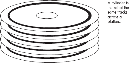
The various read/write heads are physically connected to the same actuator. Therefore, each head sits above the same track on its respective platter, and all the heads move across the disk surfaces as a unit. The set of all tracks over which the read/write heads are currently sitting is known as a cylinder (see Figure 12-10).

Figure 12-10. A hard disk cylinder

Although using multiple heads and platters increases the cost of a hard disk drive, it also increases the performance. The performance boost occurs when data that the system needs is not located on the current track. In a hard disk subsystem with only one platter, the read/write head would need to move to another track to locate the data. But in a disk subsystem with multiple platters, the next block of data to read is usually located within the same cylinder. And because the hard disk controller can quickly switch between read/write heads electronically, doubling the number of platters in a disk subsystem nearly doubles the track seek performance of the disk unit because it winds up doing half the number of seek operations. Of course, increasing the number of platters also increases the capacity of the unit, which is another reason why high-capacity drives are often higher-performance drives as well.

With older disk drives, when the system wants to read a particular sector from a particular track on one of the platters, it commands the disk to position the read/write heads over the appropriate track, and the disk drive then waits for the desired sector to rotate underneath. But by the time the head settles down, there’s a chance that the desired sector has just passed under the head, meaning the disk will have to wait for almost one complete rotation before it can read the data. On the average, the desired sector appears halfway across the disk. If the disk is rotating at 7,200 RPM (120 revolutions per second), it requires 8.333 milliseconds for one complete rotation of the platter, and, if on average the desired sector is halfway across the disk, 4.2 milliseconds will pass before the sector rotates underneath the head. This delay is known as the average rotational latency of the drive, and it is usually equivalent to the time needed for one rotation, divided by two.

To see how this can be a problem, consider that an OS usually manipulates disk data in sector-sized chunks. For example, when reading data from a disk file, the OS will typically request that the disk subsystem read a sector of data and return that data. Once the OS receives the data, it processes the data and then very likely makes a request for additional data from the disk. But what happens when this second request is for data that is located on the next sector of the current track? Unfortunately, while the OS is processing the first sector’s data, the disk platters are still moving underneath the read/write heads. If the OS wants to read the next sector on the disk’s surface and it doesn’t notify the drive immediately after reading the first sector, the second sector will rotate underneath the read/write head. When this happens, the OS will have to wait for almost a complete disk rotation before it can read the desired sector. This is known as blowing revs (revolutions). If the OS (or application) is constantly blowing revs when reading data from a file, file system performance suffers dramatically. In early “single-tasking” OSes running on slower machines, blowing revs was an unpleasant fact. If a track had 64 sectors, it would often take 64 revolutions of the disk in order to read all the data on a single track.

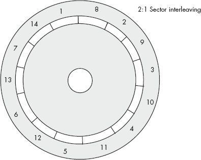
To combat this problem, the disk-formatting routines for older drives allow the user to interleave sectors. Interleaving sectors is the process of spreading out sectors within a track so that logically adjacent sectors are not physically adjacent on the disk surface (see Figure 12-11).

The advantage of interleaving sectors is that once the OS reads a sector, it will take a full sector’s rotation time before the logically adjacent sector moves under the read/write head. This gives the OS time to do some processing and to issue a new disk I/O request before the desired sector moves underneath the head. However, in modern multitasking OSes, it’s difficult to guarantee that an application will gain control of the CPU so that it can respond before the next logical sector moves under the head. Therefore, interleaving isn’t very effective in such multitasking OSes.

To solve this problem, as well as improve disk performance in general, most modern disk drives include memory on the disk controller that allows the controller to read data from an entire track. By avoiding interleaving the controller can read an entire track into memory in one disk revolution, and once the track data is cached in the controller’s memory, the controller can communicate disk read/write operations at RAM speed rather than at disk rotation speeds, which can dramatically improve performance. Reading the first sector from a track still exhibits rotational latency problems, but once the disk controller reads the entire track, the latency is all but eliminated for that track.

Figure 12-11. Interleaving sectors

A typical track may have 64 sectors of 512 bytes each, for a total of 32 KB per track. Because newer disks usually have between 512 KB and 8 MB of on-controller memory, the controller can buffer as many as 100 or so tracks in its memory. Therefore, the disk-controller cache not only improves the performance of disk read/write operations on a single track, it also improves overall disk performance. And the disk-controller cache not only speeds up read operations, but write operations as well. For example, the CPU can often write data to the disk controller’s cache memory within a few micro-seconds and then return to normal data processing while the disk controller moves the disk read/write heads into position. When the disk heads are finally in position at the appropriate track, the controller can write the data from the cache to the disk surface.

From an application designer’s perspective, advances in disk subsystem design have attempted to reduce the need to understand how disk drive geometries (track and sector layouts) and disk-controller hardware affect the application’s performance. Despite these attempts to make the hardware transparent to the application, though, software engineers wanting to write great code must always remain cognizant of the underlying operation of the disk drive. For example, sequential file operations are usually much faster than random-access operations because sequential operations require fewer head seeks. Also, if you know that a disk controller has an on-board cache, you can write file data in smaller blocks, doing other processing between the block operations, to give the hardware time to write the data to the disk surface. Though the techniques early programmers used to maximize disk performance don’t apply to modern hardware, by understanding how disks operate and how they store their data, you can avoid various pitfalls that produce slow code.

Tape drives are also popular mass storage devices. Traditionally, personal computer owners have used tape drives to back up data stored on hard disk drives. For many years, tape storage was far more cost-effective than hard disk storage on a cost-per-megabyte basis. Indeed, at one time there was an order of magnitude difference in cost per megabyte between tape storage and magnetic disk storage. And because tape drives held more data than most hard disk drives, they were more space-efficient too.

However, because of competition and technological advances in the hard disk drive marketplace, tapes have lost these advantages. Hard disk drives are now exceeding 250 GB in storage, and the optimum price point for hard disks is about $0.50 per gigabyte. Tape storage today costs far more per megabyte than hard disk storage. Plus, only a few tape technologies allow one to store 250 GB on a single tape, and those that do (such as Digital Linear Tape, or DLT) are extremely expensive. It’s not surprising that tape drives are seeing less and less use these days in home PCs and are typically found only in larger file server machines.

Back in the days of mainframes, application programs interacted with tape drives in much the same way that today’s applications interact with hard disk drives. A tape drive, however, is not an efficient random access device. That is, although software can read a random set of blocks from a tape, it cannot do so with acceptable performance. Of course, in the days when most applications ran on mainframes, applications generally were not interactive, and the CPUs were much slower. As such, the standard for “acceptable performance” was different.

In a tape drive, the read/write head is fixed, and the tape transport mechanism moves the tape past the read/write head linearly, from the beginning of the tape to the end of the tape, or vice versa. If the beginning of the tape is currently positioned over the read/write head and you want to read data at the end of the tape, you have to move the entire tape past the read/write head to get to the desired data. This can be very slow, requiring tens or even hundreds of seconds, depending on the length and format of the tape. Compare this with the tens of milliseconds it takes to reposition a hard disk’s read/write head. Therefore, to perform well on a tape drive, software has to be written with special awareness of the limitations of a sequential access device. In particular, data should be read or written sequentially on a tape to produce the highest performance.

Originally, data was written to tapes in blocks (much like sectors on a hard disk), and the drives were designed to allow quasi-random access to the tape’s blocks. If you’ve ever seen an old science fiction movie with the old-style reel-to-reel drives, with the reels constantly stopping, starting, stopping, reversing, stopping, and continuing, you were seeing “random access” in action. Such tape drives were very expensive because they required powerful motors, finely tooled tape-path mechanisms, and so on. As hard drives became larger and less expensive, applications stopped using tape as a data manipulation medium and used tape only for offline storage. Using a tape drive was simply too slow for normal application work. As a result, most systems started using tape drives only in sequential mode for backing up data from hard disks.

Because sequential data access on tape does not require the heavy-duty mechanics of the original tape drives, the tape drive manufactures sought to make a lower-cost product suitable for sequential access only. Their solution was the streaming tape drive, which was designed to keep the data constantly moving from the CPU to the tape, or vice versa. For example, while backing up the data from a hard disk to tape, a streaming tape drive treats the data like a video or audio recording and just lets the tape run, constantly writing the data from the hard disk to the tape. Because of the way streaming tape drives work, very few applications deal directly with the tape unit. Today, it’s very rare for anything other than a tape backup utility program, run by the system administrator, to access the tape hardware.

An interesting storage medium that has recently become popular because of its compact form factor ^[48] is flash storage media. The flash medium is actually a semiconductor device, based on the electrically erasable programmable read-only memory (EEPROM) technology, which, despite its name, is both readable and writable. Unlike regular semiconductor memory, flash storage is non-volatile, meaning that it maintains its data even in the absence of power. Like other semiconductor technologies, flash storage is purely electronic and doesn’t require any motors or other electro-mechanical devices for proper operation. Therefore, flash storage devices are more reliable and shock resistant, and they use far less power than mechanical storage solutions such as disk drives. This makes flash storage solutions especially valuable in portable battery-powered devices like PDAs, electronic cameras, MP3 playback devices, and portable recorders.

Flash storage modules now provide between 2 MB and several gigabytes of storage, and their optimal price point is at about $0.25 per megabyte. This makes them far more expensive per bit than hard disk storage, which means that their use as a storage medium is diminished.

Flash devices are sold in many different form factors. OEMs (original equipment manufacturers) can buy flash storage devices that look like other semiconductor chips and then mount these devices directly on their circuit boards. However, most flash memory devices sold today are built into one of several standard forms including PC Cards, CompactFlash cards, smart memory modules, memory sticks, or USB/flash modules. For example, a digital camera user might remove a CompactFlash card from their camera, insert it into a special CompactFlash card reader on their PC, and access their photographs just as they would files on a disk drive.

Memory in a flash storage module is organized in blocks of bytes, not unlike sectors on a hard disk. Unlike regular semiconductor memory, or RAM, you cannot write individual bytes in a flash storage module. Although you can generally read an individual byte from a flash storage device, to write to a particular byte you must first erase the entire block on which it resides. The block size varies by device, but most OSes will treat these flash blocks like a disk sector for the purposes of reading and writing. Although the basic flash storage device itself could connect directly to the CPU’s memory bus, most common flash storage packages (such as Compact Flash cards and Memory Sticks) contain electronics that simulate a hard disk interface, and you access the flash device just as you would a hard disk drive.

One interesting aspect to flash memory devices, and EEPROM devices in general, is that they have a limited write lifetime. That is, you may only write to a particular memory cell in a flash memory module a certain number of times before that cell begins to have problems retaining the information. In early EEPROM/flash devices, this was a big concern because the average number of write cycles before failures would begin occurring was around 10,000. That is, if some software wrote to the same memory block 10,000 times in a row, the EEPROM/flash device would probably develop a bad memory cell in that block, effectively rendering the entire chip useless. On the other hand, if the software wrote just once to 10,000 separate blocks, the device could still take 9,999 additional writes to each memory cell. Therefore, the OSes of these early devices would try to spread out write operations across the entire device to minimize damage. Although modern flash devices still exhibit this problem, technological advances have reduced it almost to the point where we can ignore it. A modern flash memory cell supports an average of about a million write cycles before it will go bad. Furthermore, today’s OSes simply mark bad flash blocks, the same way they mark bad sectors on a disk, and will skip a block once they determine that it has gone bad.

Being electronic, flash devices do not exhibit rotational latency times at all, and they don’t exhibit much in the way of seek times. There is a tiny amount of time needed to write an address to a flash memory module, but it is nothing compared to the head seek times on a hard disk. Despite this, flash memory is generally nowhere near as fast as typical RAM. Reading data from a flash device itself usually takes microseconds (rather than nanoseconds), and the interface between the flash memory device and the system may require additional time to set up a data transfer. Worse still, it is common to interface a flash storage module to a PC using a USB flash reader device, and this often reduces the average read time per byte to hundreds of micro-seconds.

Write performance is even worse. To write a block of data to flash, you must write the data, read it back, compare it to the original data, and rewrite it if they don’t match. Writing a block of data to flash can take several tens or even hundreds of milliseconds.

As a result, flash memory modules are generally quite a bit slower than high-performance hard disk subsystems. Technological advances are improving their performance, a process that is mainly being driven by high-end digital camera users who want to be able to snap as many pictures as possible in a short time. Though flash memory performance will probably not catch up with hard disk performance any time soon, it should steadily improve as time passes.

Another pair of interesting mass storage devices you’ll find are the RAM and semiconductor disks. A RAM disk is just an application that treats a large block of the computer system’s memory as though it were a disk drive, simulating blocks and sectors using memory arrays. A semiconductor disk is a device consisting of RAM memory and a controller that interfaces with the system using a traditional disk interface. Semiconductor disks usually have their own power supply (including a battery backup system) so that they maintain memory integrity when you turn off the PC. The use of a standard disk interface and a separate, uninterruptible, power supply are what differentiate true semiconductor disks from software-based RAM disks.

The advantage of memory-based disks is that they are very high performance. RAM disks and semiconductor disks do not exhibit the time delays associated with head seek time and rotational latency that you find on hard, optical, and floppy drives. Their interface to the CPU is also much faster, so data transfer times are very high, often running at the maximum bus speed. It is hard to imagine a faster storage technology than a RAM or semiconductor disk.

RAM and semiconductor disks, however, have two disadvantages: cost and volatility. The cost per byte of storage in a semiconductor disk system is very high. Indeed, byte-for-byte, semiconductor storage is as much as 1,000 times more expensive than magnetic hard disk storage. Because of the high cost of semiconductor storage, semiconductor disks usually have low storage capacities, typically no more than a couple of gigabytes. And, semiconductor disks are volatile — they lose their memory unless they are powered at all times. A battery-backed, uninterruptible power supply can help prevent memory loss during power failures, but you cannot disconnect a semiconductor disk from the power line for an extended period of time and expect the data to persist. This generally means that semiconductor disks are great for storing temporary files and files you’ll copy back to some permanent storage device before shutting down the system. Because of their low-latency, high data transfer rates, and relatively low storage capacity, semiconductor disks are excellent for use as swap storage for a virtual memory subsystem. They are not particularly well suited for maintaining important information over long periods of time.

The popularity of semiconductor disks tends to rise and fall with mother-board and CPU designs. Semiconductor disks tend to be more popular when it is physically impossible to extend the amount of memory in a given computer system. Semiconductor disks tend to be less popular when a computer system allows memory expansion. The reason for this is simple: It is far less expensive to increase the RAM in a typical computer system and use a soft-ware-based RAM disk than it is to add a semiconductor disk to the system. A software-based RAM disk is usually faster than a semiconductor disk because the system can access the RAM disk at memory bus speeds rather than at disk controller speeds. In fact, there are only two disadvantages to RAM disks: their memory is volatile, and every byte you allocate to a RAM disk is one less byte available for your applications. In a few systems, these two disadvantages prevent the use of RAM disks. For most uses, however, if there is a little extra unused RAM in the system, and the user is careful to copy important data from the RAM disk to nonvolatile storage before shutting off the system, a software-based RAM disk can be a very cost-effective solution.

The problems with software-based RAM disk solutions begin when you have added all the RAM your system can support, and your applications require most of the memory in the system. Back when CPUs had a 16-bit address space, users quickly reached the point where they had installed as much as 64 KB of memory on their machines (2¹⁶ bytes is 64 KB). When the 8088/8086 rolled around with a 20-bit address bus, it wasn’t long before users had installed the maximum amount of memory in those machines too. Ditto for CPUs with a 24-bit address bus, allowing a maximum of 16 MB of memory. Once CPUs started supporting 32-bit address buses, it seemed like the amount of memory one could install in the system had hit infinity, but today we’re once again bumping up against that limit. It’s not uncommon now to find machines with the maximum amount of memory already installed, particularly since motherboards often limit the amount of RAM that can be installed on a system even though the system CPU can address a much larger amount of RAM.

Semiconductor disks become practical when you’ve installed the maximum amount of RAM in your system and the applications or OS are making use of that memory, so that there isn’t a large block of memory lying around that you can use for a RAM disk. Because the semiconductor disk’s memory exists outside the CPU’s address space, it does not impact the memory limits that apply to motherboard designs.

The Small Computer System Interface (SCSI, pronounced “scuzzy”) is a peripheral interconnection bus used to connect high-speed peripheral devices to personal computer systems. Designed in the early 1980s, the SCSI bus was popularized by its introduction on the Apple Macintosh computer system in the middle 1980s. The original SCSI interface supported an 8-bit bidirectional data bus and was capable of transferring 5 MB of data per second, which was considered “high-performance” for hard disk subsystems of that era. Although the performance of that early SCSI interface is quite slow by modern standards, SCSI has gone through several revisions over the years and remains a high-performance peripheral interconnection system. Today’s SCSI devices are capable of transferring 320 MB per second.

Although the SCSI interconnection system is most commonly used for disk drive subsystems, SCSI was designed to support a whole host of PC peripherals using a cable connection. Indeed, as SCSI became popular during the late 1980s and into the 1990s, you could find printers, scanners, imaging machines, phototypesetters, network, and display adapters, and many other devices interfacing with the SCSI bus. However, the popularity of the SCSI bus as a general-purpose peripheral bus has diminished since the appearance of the USB and FireWire peripheral connection systems. Except for very high performance disk drive subsystems and some very specialized peripheral devices, few new peripherals use the SCSI interface.

To understand why SCSI’s popularity is waning, one must consider the problems SCSI users have faced over the years. When SCSI was first introduced, the SCSI bus supported concurrent connection of the SCSI adapter card and up to seven actual peripheral devices. To connect multiple devices, one first ran a cable from the host controller card to the first peripheral device. To connect a second device, one ran a cable from a second connector on the first device to the second device. To connect a third device, one ran a cable from a separate connector on the second device to the third device, and so on. At the end of this “daisy chain” of devices, one attached a special terminating device to the last connector of the last peripheral device. Without the special “terminator” at the end of the SCSI chain, many SCSI systems would work unreliably, if at all.

As a “convenience” to their customers, many peripheral manufacturers built the terminating circuitry into their devices. Unfortunately, connecting multiple terminators in the middle of the SCSI chain was just as bad as not having a terminator in the SCSI system. Though most manufacturers who designed the terminating circuitry into their peripherals often provided an option to disable the terminator, some did not. Ensuring that those devices with the active terminator circuitry were at the end of the SCSI chain was often cumbersome, and even if a device provided an option to enable or disable the terminator, knowing the appropriate “dip-switch” settings was a problem if the documentation wasn’t handy. As a result, many computer owners had problems with a chain of SCSI devices not working properly in their system.

On the original SCSI bus, the computer system owner had to assign each device one of eight numeric “addresses” from zero to seven, with address seven generally reserved for the host controller card. If two devices in the SCSI chain had the same address, they wouldn’t operate properly. This made moving SCSI peripherals from one computer system to another somewhat difficult, because the address of the device being moved was usually already taken by another device on the new system.

The original SCSI bus had other limitations as well. First, it only supported seven peripheral devices. When SCSI was first designed, this wasn’t usually a problem because common SCSI peripherals like hard drives and scanners were very expensive, costing thousands of dollars each. Connecting more than seven devices wasn’t something your average computer owner would have done back then. But, as the price of hard drives and other SCSI peripherals came down, the seven-peripheral limit became burdensome. Second, SCSI was not, and still is not, hot swappable. That is, you cannot unplug a peripheral device while power is applied to the system, nor may you connect a new peripheral to the SCSI bus while the power is on. Doing so could cause electrical damage to the SCSI controller, the peripheral, or even some other peripheral on the SCSI bus. As SCSI peripherals came down in price and people began connecting multiple devices to their computer systems, the desire to unplug a device from one system and plug it into another grew, but SCSI did not support this mode of operation.

Despite all these bad features, SCSI’s popularity grew. To maintain that popularity, SCSI was modified over time to improve its functionality. SCSI-2, the first modification, doubled the speed from 5 MHz to 10 MHz, thus doubling the data transfer rate on the bus. This was necessary because the speed of high-performance devices like disk drives increased so much that the original SCSI interface was actually slowing them down. The next improvement was to increase the size of the bidirectional SCSI data bus from 8 bits to 16 bits. This not only doubled the data transfer rate from 10 MB per second to 20 MB per second, it also increased the number of peripherals one could place on the bus from 7 to 15. Variations of SCSI-2 were known as Fast SCSI (10 MHz), Wide SCSI (16 bits), and Fast and Wide SCSI (16 bits at 10 MHz).

It should come as no surprise that SCSI-3 followed SCSI-2. SCSI-3 offers a veritable smorgasbord of different connection options while maintaining compatibility with the older standards. Although SCSI-3 (using names like Ultra, Ultra Wide, Ultra2, Wide Ultra2, Ultra3, and Ultra320) still operates as a 16-bit bus in the parallel cable mode, and it still supports a maximum of 15 peripherals, it is vastly improved. SCSI-3 increased the operating speed of the bus and the maximum permissible physical distance across which SCSI peripherals could be chained. To make a long story short, SCSI-3 operates at speeds of up to 160 MHz, allowing the SCSI bus to transfer data in bursts up to 320 MB per second (that is, faster than many PCI bus interconnects!).

SCSI was originally a parallel interface. Today, SCSI supports three different interconnection standards: SCSI Parallel Interface (SPI), Serial SCSI across FireWire, and Fibre Channel Arbitrated Loop. The SPI is the original definition that most people associate with the SCSI interface. SCSI parallel cables contain either 8 or 16 data lines, depending on the type of SCSI interface in use. This makes SCSI cables bulky, heavy, and expensive. The parallel SCSI interface also limits the maximum length of the SCSI chain in the system to just a few meters. These concerns, especially the economic ones, are why modern computer systems only use SCSI peripherals when extremely high performance is necessary.

An important fact to note about SCSI is that it is not a master/slave interconnection system. That is, the computer system does not own the bus and doesn’t necessarily direct the traffic between various peripherals on the bus. SCSI is a true peer-to-peer bus, and any two peripherals on the bus may communicate with one another. Indeed, it’s possible (though unusual) for two computer systems to share the same SCSI bus. This peer-to-peer operation can improve the performance of the overall system tremendously. To illustrate this point, consider a tape backup system. In practice, most tape backup programs read a block of data from a disk drive into the computer’s memory and then write that block of data from the computer’s memory to the tape drive. On the SCSI bus (in theory, at least), it is possible to have the tape and disk drives communicate directly with one another. The tape backup software would send two commands, one to the disk drive and one to the tape drive, telling the disk drive to transfer the block of data directly to the tape drive rather than going through the computer system. Not only does this reduce the number of transfers across the SCSI bus by half, speeding up the transfer, but it also frees up the computer’s CPU to do other things. In reality, few tape backup systems work this way, but there are many examples where two peripherals communicate with one another across the SCSI bus without using the computer as an intermediary. Software that programs SCSI peripherals to operate this way (rather than running the data through the computer’s memory) is a good example of great programming.

SCSI is interesting insofar as it is not only an electrical interconnection, but a protocol as well. One does not communicate with a SCSI peripheral device by writing some data to a couple of registers on the SCSI interface card, causing that data to travel down the SCSI cable to the peripheral device. Although SCSI is a parallel interface like the parallel printer port, it doesn’t communicate with SCSI peripheral devices like the parallel port communicates with printer devices. To use SCSI, you build up a data structure in memory containing a SCSI command, command parameters, any data you may want to send to the SCSI peripheral, and possibly a pointer with the memory address where the SCSI controller should store any data the peripheral device returns. Once you construct this data structure, you normally provide the SCSI controller with the data structure’s address, and the SCSI controller then fetches the command from system memory and sends it to the appropriate peripheral device on the SCSI bus.

As SCSI hardware has evolved over the years, so has the SCSI protocol, the SCSI command set. SCSI was never intended to serve as just a hard disk interface, and the breadth of peripherals that SCSI supports has steadily increased over the years along with the advent of new types of computer peripherals. To accommodate these new and unanticipated uses for the SCSI bus, SCSI’s designers created a device-independent command protocol that could be easily extended as new devices were invented. Contrast this with certain device interfaces such as the original Integrated Disk Electronics (IDE) interface, which was suitable only for disk drives.

The SCSI protocol transmits a packet containing the peripheral’s address, the command, and the command’s data. The SCSI-3 standard has roughly grouped these commands into the following classes:

What do these commands look like? Unlike traditional interfaces such as serial and parallel, one does not necessarily write SCSI “commands” to registers on the SCSI controller chip. Indeed, SCSI commands are generally intended for devices on the SCSI bus, not for the SCSI host controller (which is often called the SCSI host adapter). The job of the host controller, from the programmer’s perspective, is to place SCSI commands onto the SCSI bus for use by other peripherals and to fetch commands and data from the SCSI bus intended for the host system. Although the SCSI commands themselves are standardized, the actual interface to the SCSI host controller is not. Different host controller manufacturers use different hardware to connect their SCSI controller chips to the host computer system, so how you talk to a SCSI controller chip is different, depending on the particular host controller device. Because SCSI controllers are very complex and difficult to program, and because there is no “standard” SCSI interface chip, programmers are faced with having to write several different variants of their software to control SCSI devices.

To correct this situation, SCSI host controller manufacturers like Adaptec have created specialized device driver modules that provide a uniform interface to their devices. Rather than writing data directly to a SCSI chip, a programmer creates an in-memory data structure with SCSI commands to be placed on the SCSI bus, calls the device driver software, and lets the device driver transfer the SCSI commands to the SCSI bus. There are several nice things about this approach:

This concept was carried forward into modern OSes. Today, SCSI host controller manufacturers write SCSI miniport drivers for OSes like Windows. These miniport drivers provide a hardware-independent interface to the host controller so that the OS can simply say, “Here is a SCSI command. Put it on the SCSI bus.”

One big advantage of the SCSI interface is that it provides parallel processing of SCSI commands. That is, a host system can place several different SCSI commands on the bus, and different peripheral devices can process those commands simultaneously. Some devices, like disk drives, can even accept multiple commands at once and process those commands in the order that is most efficient. As an example, suppose that a disk drive is currently near block 1,000. If the system sends block read requests for blocks 5,000; 4,560; 3,000; and 8,000; the disk controller can rearrange these requests and satisfy them in the most efficient order (probably 3,000; 4,560; 5,000; and then 8,000) as it moves the read/write head across the surface of the disk. This results in a big performance improvement on multitasking OSes that process requests for disk I/O from several different applications simultaneously.

SCSI is also a great interface for RAID systems because SCSI is one of the few disk controller interfaces that supports a large number of drives on the same interface. Indeed, because no modern hard drive is capable of equaling SCSI data transfer rates, the only way to achieve SCSI’s 320-MB-per-second transfer rate is with a RAID subsystem. Very high performance drives are capable of sustaining only about 80-MB-per-second data transfer rates, and that’s only in burst mode. In an ideal world where the SCSI protocol did not consume any overhead, you would have to connect four such drives to a RAID/SCSI controller to achieve the theoretical maximum data transfer rate on the SCSI bus.^[49] A very high performance RAID controller would sit between the SCSI bus and the actual hard drives. Lower-cost RAID systems can be created by connecting the disks directly to the SCSI bus and using special software to send disk I/O operations to different disks on the SCSI bus. Such systems don’t require special hardware, but they don’t achieve the maximum throughput that is possible on SCSI either; not that they run particularly slowly, mind you.

The SCSI command set is very powerful, and it is designed for high-performance applications. It is sufficiently large and complex that space limitations prevent its inclusion here. Readers interested in a deeper look at SCSI programming should refer to The Book of SCSI (by Gary Field, Peter M. Ridge, et al., published by No Starch Press). The complete SCSI specifications appear at various sites on the Web. A quick search for “SCSI specifications” on AltaVista, Google, or any other decent Web search engine should turn up several copies of the specifications.

Although the SCSI interface is very high performance, it is also expensive. A SCSI device requires a sophisticated and fast processor in order to handle all the operations that are possible on the SCSI bus. Furthermore, because SCSI devices can operate on a peer-to-peer basis (that is, one peripheral may talk to another without intervention from a host computer system), each SCSI device must carry around a considerable amount of sophisticated software in ROM on the device’s controller board. Adding all the extra functionality needed to support full SCSI when all you want to do is to attach a single hard disk to a personal computer system is a bit of overkill. During the middle to late 1980’s, several computer and disk manufacturers got together to discuss a less expensive, though standardized, interface that would let them connect inexpensive disk drives to personal computers. The result of this initiative was the IDE (Integrated Drive Electronics) interface.

The point behind SCSI was to off load as much work as was reasonably possible to the device controller, freeing up the host computer to do other activities. But all this extra complexity and cost to improve system performance was going to waste because in typical personal computer systems the host computer was usually waiting for the data transfer to complete. So the computer was sitting idle while the SCSI disk drive was busy processing the SCSI command. The idea behind the IDE interface was to lower the cost of the disk drive by using the host computer’s CPU to do the processing. Because the CPU was usually idle (during SCSI transfers) anyway, this seemed like a good use of resources. IDE drives, because they were often hundreds of dollars less than SCSI drives, became incredibly popular on personal computer systems.

The original IDE drive specification was very limited compared to the SCSI interface. First, it supported only two drives chained together (modern systems provide two IDE interfaces, a primary channel and a secondary channel, that support up to four devices). Second, the IDE specification was created only for disk drives; it was not a general-purpose peripheral interface bus like SCSI. And third, cable lengths for the IDE interface effectively limited IDE devices to residing in the same case as the CPU. Nevertheless, the much lower cost of the IDE interface and of IDE drives ensured its popularity.

Soon after the introduction of the IDE interface, peripheral manufacturers discovered that there were other devices that they’d like to connect to the IDE interface. Though the IDE interface was designed specifically for mass storage devices, and wouldn’t work well with non-storage devices like scanners and printers, there were many types of storage devices other than hard disks (such as CD-ROMs, tape drives, and Zip drives) for which the IDE interface represented a cheap alternative to SCSI. Furthermore, because most PCs were being shipped with IDE interfaces, manufacturers of non-hard-disk mass storage devices were drooling over the possibility of connecting to an interface found on all new personal computer systems. Because the original IDE specification was geared specifically to hard disk drives and was not particularly well suited for other types of storage devices, the committee that designed the IDE interface went back to work and developed the AT Attachment with Packet Interface (IDE/ATAPI), which is usually shortened to ATA (Advanced Technology Attachment). Like SCSI, the ATA standard has gone through several revisions and improvements over the years.

Originally, IDE was designed to work on a 33-MHz PCI bus and was theoretically capable of transferring 33 MB per second. Later revisions of the ATA standard (ATA-66, ATA-100, and ATA-133) were capable of transferring data at 66 MB, 100 MB, and 133 MB per second. One might think that with these speeds (which far outstrip the speed of the physical disk drives) the ATA interface would be comparable to SCSI in performance. However, there are two reasons why the ATA interface is still slower than SCSI. First, the host processor is still involved in many of the operations, and it may take several host computer operations across the IDE/ATA interface to accomplish what a SCSI device could do on its own. Second, SCSI supports RAID much better than the ATA interface does. For the average home user, though, the modern IDE/ATA interface provides very good performance. One easy way to compare ATA and SCSI is to note that the most recent ATA specification tends to have performance equal to the previous SCSI generation.

The ATAPI specification (in its sixth version as of December 2001) extends the IDE specification to support a wide range of mass storage devices, including tape drives, Zip drives, CD-ROMs, DVDs, removable cartridge drives, and more. In order to extend the IDE interface to support all these different storage devices, the designers of the ATAPI specification adopted a packet command format that is very similar to, and in some cases is identical to, the SCSI packet command format. One big difference between SCSI and ATA is the fact that the hardware interface for ATA is far more standardized. This allows, for example, a single BIOS routine to boot from an IDE device regardless of who manufactured the interface chip. Indeed, the major differences between various IDE/ATAPI interface chips are simply the particular ATAPI specification to which the chip adheres: ATAPI-2, ATAPI-3, ATAPI-4, ATAPI-5, or ATAPI-6. So, in theory at least, it’s possible for application programmers to communicate directly with the IDE/ATAPI interface and control the mass storage device directly.

In modern protected-mode OSes like Windows or Linux, however, an application programmer is never allowed to talk directly to the hardware. In theory, it would be possible to write a miniport driver for IDE to simulate the way the SCSI interface works. In practice, however, the OS vendor generally supplies a software library that provides an API (application programming interface) to the IDE/ATAPI devices. The application programmer can then make function calls to the API, passing appropriate parameters, and the underlying library routines take care of the remaining tasks associated with actually talking to the hardware.

Programming ATAPI devices in a modern system is quite similar to programming SCSI devices. You load up a memory-based data structure with a command code and a set of parameters, and then pass the memory structure to a driver library function that passes the data across the ATAPI interface to the target storage device. If such a low-level library is not available, and your OS allows it, you can program the ATAPI interface device to grab this data (generally using DMA on modern systems). The full ATAPI-6 specification is almost 500 pages long; obviously, we do not have sufficient space to cover the specification in any kind of detail. If you are interested in a more detailed look at the IDE/ATAPI specifications, search for “ATAPI specifications” with your favorite Internet search engine.

Modern machines use a serial ATA (SATA) controller. This is a high-performance serial version of the venerable IDE/ATAPI parallel interface. However, to the programmer, SATA looks exactly like ATAPI.

Very few applications access mass storage devices directly. That is, applications do not generally read and write tracks, sectors, or blocks on a mass storage device. Instead, most applications open, read, write, and otherwise manipulate files on the mass storage device. The OS’s file manager is responsible for abstracting away the physical configuration of the underlying storage device and providing a convenient storage facility for multiple independent files on a single device.

On the earliest computer systems, application software was responsible for tracking the physical position of data on a mass storage device because there was no file manager available to handle this function for them. Such applications were able to maximize their performance by carefully considering the layout of data on the disk. For example, software could manually interleave data across various sectors on a track to give the CPU time to process data between reading and writing those sectors on the track. Such software was often many times faster than comparable software using a generic file manager. Later, when file managers were commonly available, some application authors still managed their files on a storage device for performance reasons. This was especially true back in the days of floppy disks, when low-level software written to manipulate data at the track and sector level often ran ten times faster than the same application using a file manager system.

In theory, today’s software could benefit from this as well, but you rarely see such low-level disk access in modern software for several reasons. First, writing software that manipulates a mass storage device at such a low level locks you into using that one particular device. That is, if your software manipulates a disk with 48 sectors per track, 12 tracks per cylinder, and 768 cylinders per drive, that same software will not work optimally (if at all) on a drive with a different sector, track, and cylinder layout. Second, accessing the drive at a low level makes it difficult to share the device among different applications, something that can be especially costly on a multitasking system that may have multiple applications sharing the device at once. For example, if you’ve laid out your data on various sectors on a track to coordinate computation time with sector access, your work is lost when the OS interrupts your program and gives some other application its timeslice, thus consuming the time you were counting on to do any computations prior to the next data sector rotating under the read/write head. Third, some of the features of modern mass storage devices, such as on-board caching controllers and SCSI interfaces that present a storage device as a sequence of blocks rather than as something with a given track and sector geometry, eliminate any advantage such low-level software might have had at one time. Fourth, modern OSes typically contain file buffering and block caching algorithms that provide good file system performance, obviating the need to operate at such a low level. Finally, low-level disk access is very complex and writing such software is difficult.

The earliest file manager systems stored files sequentially on the disk’s surface. That is, if each sector/block on the disk held 512 bytes and a file was 32 KB long, that file would consume 64 consecutive sectors/blocks on the disk’s surface. In order to access that file at some future time, the file manager only needed to know the file’s starting block number and the number of blocks it occupied. Because the file system had to maintain these two pieces of information somewhere in nonvolatile storage, the obvious place was on the storage media itself, in a data structure known as the directory. A disk directory is an array of values starting at a specific location on the disk that the OS can reference when an application requests a specific file. The file manager can search through the directory for the file’s name and extract its starting block and length. With this information, the file system can provide the application with access to the file’s data.

One advantage of the sequential file system is that it is very fast. The OS can read or write a single file’s data very rapidly if the file is stored in sequential blocks on the disk’s surface. But a sequential file organization has some big problems, too. The biggest and most obvious drawback is that you cannot extend the size of a file once the file manager places another file at the next block on the disk. Disk fragmentation is another big problem. As applications create and delete many small and medium-sized files, the disk fills up with small sequences of unused sectors that, individually, are too small for most files. It was common on sequential file systems to find disks that had sufficient free space to hold some data, but that couldn’t use that free space because it was spread all over the disk’s surface in small pieces. To solve this problem, users had to run disk compaction programs to coalesce all the free sectors and move them to the end of the disk by physically rearranging files on the disk’s surface. Another solution was to copy files from one full disk to another empty disk, thereby collecting the many small, unused sectors together. Obviously, this was extra work that the user had to do, work that the OS should be doing.

The sequential-file storage scheme really falls apart when used with multitasking OSes. If two applications attempt to write file data to the disk concurrently, the file system must place the starting block of the second application’s file beyond the last block required by the first application’s file. As the OS has no way of determining how large the files can grow, each application has to tell the OS the maximum length of the file when the application first opens the file. Unfortunately, many applications cannot determine, beforehand, how much space they will need for their files. So the applications have to guess the file size when opening a file. If the estimated file size is too small, either the program will have to abort with a “file full” error, or the application will have to create a larger file, copy the old data from the “full” file to the new file, and then delete the old file. As you can imagine this is horribly inefficient, and definitely not great code.

To avoid such performance problems, many applications grossly over-estimate the amount of space they need for their files. As a result, they wind up wasting disk space when the files don’t actually use all the data allocated to them, a form of internal fragmentation. Furthermore, if applications truncate their files when closing them, the resulting free sections returned to the OS tend to fragment the disk into small, unusable blocks of free space, a problem known as external fragmentation. For these reasons, sequential storage on the disk was replaced by more sophisticated storage-management schemes in modern OSes.

Most modern file-allocation strategies allow files to be stored across arbitrary blocks on the disk. Because the file system can now place bytes of the file in any free block on the disk, the problems of external fragmentation and the limitation on file size are all but eliminated. As long as there is at least one free block on the disk, you can expand the size of any file. However, along with this flexibility comes some extra complexity. In a sequential file system, it was easy to locate free space on the disk — by noting the starting block numbers and sizes of the files in a directory, it was possible to easily locate a free block large enough to satisfy the current disk allocation request, if such a block was available. But with a file system that stores files across arbitrary blocks, scanning the directory and noting which blocks a file uses is far too expensive to compute, so the file system has to keep track of the free and used blocks. Most modern OSes use one of three data structures — a set, a table (array), or a list — to keep track of which sectors are free and which are not. Each of these schemes has its advantages and disadvantages, and you’ll find all three schemes in use in modern OSes.

12.21.3 List-of-Blocks File Organization

To overcome the limitations of the FAT file system, advanced OSes such as Windows NT/2000/XP and various flavors of Unix use a list-of-blocks scheme rather than a FAT. Indeed, the list scheme enjoys all the advantages of a FAT system (such as efficient, nonlinear free-block location, and efficient storage of the free-block list), and it solves many of FAT’s problems.

The list scheme begins by setting aside several blocks on the disk for the purpose of keeping (generally) 32-bit pointers to each of the free blocks on the disk. If each block on the disk holds 4,096 bytes, a block can hold 1,024 pointers. Dividing the number of blocks on the disk by 1,024 determines the number of blocks the free-block list will initially consume. As you’ll soon see, the system can actually use these blocks to store data once the disk fills up, so there is no storage overhead associated with the blocks consumed by the free-block list.

If a block in the free-block list contains 1,024 pointers, then the first 1,023 pointers contain the block numbers of free blocks on the disk. The file manager maintains two pointers on the disk: one that holds the block number of the current block containing free-block pointers, and one that holds an index into that current block. Whenever the file system needs a free block, it obtains the index for one from the free list block by using these two pointers. Then the file manager increments the index into the free-block list to the next available entry in the list. When the index increments to 1,023 (the 1,024th item in the free-block list), the OS does not use the pointer entry value at index 1,023 to locate a free block. Instead, the file manager uses this pointer as the address of the next block containing a list of free-block pointers on the disk, and it uses the current block, containing a now-empty list of block pointers, as the free block. This is how the file manager reuses the blocks originally designated to hold the free-block list. Unlike the FAT, the file manager does not reuse the pointers in the free-block list to keep track of the blocks belonging to a given file. Once the file manager uses up all the free-block pointers in a given block, the file manager uses that block for actual file data.

Unlike the FAT, the list scheme does not merge the free-block list and the file list into the same data structure. Instead, a separate data structure for each file holds the list of blocks associated with that file. Under typical Unix and Linux file systems, the directory entry for the file actually holds the first 8 to 16 entries in the list (see Figure 12-12). This allows the OS to track short files (up to 32 KB or 64 KB) without having to allocate any extra space on the disk.

Figure 12-12. Block list for small files

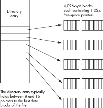
OS research on various flavors of Unix suggests that the vast majority of files are small, and embedding several pointers into the directory entry provides an efficient way to access small files. Of course, as time passes, the average file size seems to increase. But as it turns out, block sizes tend to increase as well. When this average file size research was first done, the typical block size was 512 bytes, but today a typical block size is 4,096 bytes. During that time, then, average file sizes could have increased by a factor of eight without, on average, requiring any extra space in the directory entries.

For medium sized files up to about 4 MB, the OS will allocate a single block with 1,024 pointers to the blocks that store the file’s data. The OS continues to use the pointers found in the directory entry for the first few blocks of the file, and then it uses a block on the disk to hold the next group of block pointers. Generally, the last pointer in the directory entry holds the location of this block (see Figure 12-13).

Figure 12-13. Block list for medium-sized files

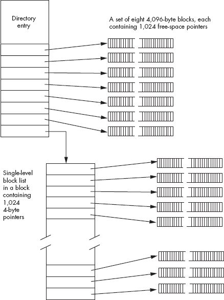
For files larger than about 4 MB, the file system switches to a three-tiered block scheme, which works for file sizes up to 4 GB. In this scheme, the last pointer in the directory entry stores the location of a block of 1,024 pointers, and each of the pointers in this block holds the location of an additional block of 1,024 pointers, with each pointer in this block storing the location of a block that contains actual file data. See Figure 12-14 for the details.

Figure 12-14. Three-level block list for large files (up to 4 GB)

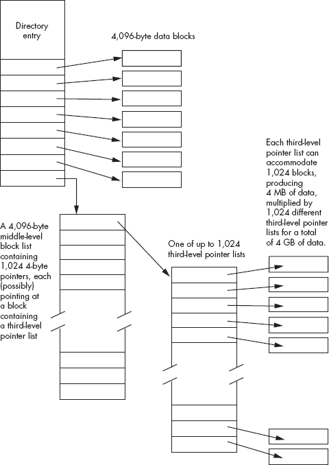
One advantage to this tree structure is that it readily supports sparse files. That is, an application can write to block 0 and block 100 of a file without having to allocate data blocks for every block in between those two points. By placing a special block pointer value (typically zero) in the intervening entries in the block list, the OS can determine whether a block is not present in the file. Should an application attempt to read such a missing block in the file, the OS can simply return all zeros for the empty block. Of course, once the application writes data to a block that hadn’t been previously allocated, the OS must copy the data to the disk and fill in the appropriate block pointer in the block list.

As disks became larger, the 4 GB file limit imposed by this scheme began to create some problems for certain applications, such as video editors, large database applications, and Web servers. One could easily extend this scheme 1,000 times — to 4 terabytes (TB) — by adding another level to the block-list tree. The only problem with this approach is that the more levels of indirection you have, the slower random file access becomes, because the OS may have to read several blocks from the disk in order to get a single block of data. (When it has one level, it is practical to cache the block-pointer list in memory, but with two and three levels, it is impractical to do this for every file). Another way to extend the maximum value size 4 GB at a time is to use multiple pointers to second-tier file blocks (for example, take the original 8 to 16 pointers in the directory and have all or most of them point at second-tier block list entries rather than directly at file data blocks). Although there is no current standard way to extend beyond three levels, rest assured that as the need arises, OS designers will develop schemes they can use to access large files in an efficient manner.

Understanding how different mass storage devices behave is important if you want to write high-performance software that manipulates files on these devices. Although modern OSes attempt to isolate applications from the physical realities of mass storage, an OS can only do so much for you. Furthermore, an OS cannot predict how your particular application will access files on a mass storage device, so the OS cannot optimize access for your specific application; instead, the OS optimizes file access for applications that exhibit typical file-access patterns. The less typical your application’s file I/O is, the less likely you’ll get the best performance out of the system. In this section, we’ll look at how you can coordinate your file access activities with the OS to achieve the best performance.

FILE *f;
int array[16];
    . . .
// Sequence #1:

fwrite( f, array, 16 * sizeof( int ));
    . . .
// Sequence #2:

for( i=0; i < 16; ++i )
    fprintf( f, "%d ", array[i] );

The Universal Serial Bus (USB) is not a peripheral port in the traditional sense (like an RS-2323 serial communications controller). Rather than using it to connect your computer to some peripheral device, USB is a mechanism that allows you to use a single interface to connect a wide variety of different peripheral devices to a PC, similar to SCSI. The USB supports hot-pluggable devices, meaning that you can plug and unplug devices without shutting down the power or rebooting your machine, and it supports plug-and-play devices, meaning that the OS will automatically load a device driver, if available, once you plug in a device. This flexibility comes at a cost, however. Programming devices on the USB is considerably more complex than programming a serial or parallel port. You cannot communicate with USB peripherals by reading or writing a few device registers.

Along with disk drives, keyboards, and display devices, pointing devices are probably the most common peripherals you’ll find on modern personal computers. Pointing devices are actually among the more simple peripheral devices, providing a very simple data stream to the computer. Pointing devices generally come in two categories: those that return the relative position of the pointer and those that return the absolute position of the pointing device. A relative position is simply the change in position since the last time the system read the device; an absolute position is some set of coordinate values within a fixed coordinate system. Mice, trackpads, and trackballs are examples of devices that return relative coordinates; touch screens, light pens, pressure-sensitive tablets, and joysticks are examples of devices that return absolute coordinates. Generally, it’s easy to translate an absolute coordinate system to a relative one, but a bit more problematic to convert a relative coordinate system to an absolute one. This latter conversion requires a constant reference point that may become meaningless if, for example, someone lifts a mouse off the surface and sets it down elsewhere. Fortunately, most windowing systems work with relative coordinate values from pointing devices, so the limitations of pointing devices that return relative coordinates are not a problem.

Early mice were typically opto-mechanical devices that rotated two encoding wheels that were oriented along the X- and Y-axes of the mouse body. Usually, both of these wheels were encoded to send 2-bit pulses whenever they would move a certain distance. One bit told the system that the wheel had moved a certain distance, and the other bit told the system which direction the wheel had moved.^[51] By constantly tracking the four bits (two bits for each axis) from the mouse, the computer system could determine the mouse’s distance and direction traveled, and keep a very accurate calculation of the mouse’s position in between application requests for that position.

One problem with having the CPU track each mouse movement is that when moved quickly, mice can generate a constant and high-speed stream of data. If the system is busy with other computations, it might miss some of the incoming mouse data and would therefore lose track of the mouse’s position. Furthermore, using the host CPU to keep track of the mouse position consumes CPU time that could be put to better use doing application computations.

As a result, mouse manufacturers decided early on to incorporate a simple microcontroller in the mouse package. This simple microcontroller keeps track of the physical mouse movements and responds to system requests for mouse coordinate updates, or at the very least generates interrupts on a periodic basis when the mouse position changes. Most modern mice connect to the system via the USB and respond with positional updates to system requests that occur about every eight milliseconds.

Because of the wide acceptance of the mouse as a GUI pointing device, computer manufacturers have created many other devices that serve the same purpose. The motivation behind developing most of these devices has been to increase portability — mice aren’t the most convenient pointing devices to attach to a laptop computer system on the road. Trackballs, strain gauges (the little “stick” you’ll find between the G and H keys on many laptops), trackpads, trackpoints, and touch screens are all examples of devices that manufacturers have attached to portable computers and PDAs to create more portable pointing devices. Though these devices vary with respect to their convenience to the end user, to the OS they can all look like a mouse. So, from a software perspective, there is little difference between these devices.

In modern OSes, the application rarely interfaces with a pointing device directly. Instead, the OS is responsible for tracking the mouse position and updating cursors and other mouse effects in the system. The OS typically notifies an application when some sort of pointing device event occurs that the application should consider. Though applications may query the pointing device’s status, as a normal state of affairs they don’t manage the pointing device’s position. In response to a query from an application, the OS will return the position of the system cursor and the state of the buttons on the pointing device. The OS may also notify the application whenever a pointer device event, such as a button press, occurs.

The analog game adapter created for the IBM PC allowed users to connect up to four resistive potentiometers and four digital switch connections to the PC. The design of the PC’s game adapter was obviously influenced by the analog input capabilities of the Apple II computer, the most popular computer available at the time the PC was developed. IBM’s analog input design, like Apple’s, was designed to be dirt-cheap. Accuracy and performance were not a concern at all. In fact, you can purchase the electronic parts to build your own version of the game adapter, at retail, for less than three dollars. Unfortunately, IBM’s low-cost design in 1981 produces some major performance problems for high-speed machines and high-performance game software in the 2000s.

Few modern systems incorporate the original electronics of the IBM PC game controller because of the inherent inefficiencies of reading them. Rather, most modern game controllers contain the analog electronics that convert physical position into a digital value directly inside the controller, and then interface to the system via USB. Microsoft Windows and other modern OSes provide a special game-controller device-driver interface that allows applications to determine what facilities the game controller has and also sends the data to those applications in a standardized form. This allows game-controller manufacturers to provide many special features that were not possible when using the original PC game-controller interface. Modern applications read game-controller data just as though they were reading data from a file or some other character-oriented device like a keyboard. This vastly simplifies the programming of such devices while improving overall system performance.

Microsoft Windows also provides a special game controller API that provides a high-performance interface to various types of game controllers on the system. Similar library modules exist for other OSes as well. Some “old-time” game programmers feel that calling such code is inherently inefficient and that great code always controls the hardware directly. This concept is a bit outdated. First, most modern OSes don’t allow applications direct access to hardware even if the programmer wants such access. Second, software that talks directly to the hardware won’t work with as wide a variety of devices as software that lets the OS handle the hardware for it. Back in the days when there were a small number of standardized peripherals for the PC, it was possible for a single application to directly program all the different devices the program would access. In modern systems, however, there are far too many devices for an individual program to deal with. This is just as true for game-controller devices as it is for other types of devices. Finally, keep in mind that most OS device drivers are probably going to be written more efficiently by the manufacturer’s programmers or the OS developer’s programmers than you could write them yourself.

Because newer game controllers are no longer constrained by the design of the original IBM PC game-controller card, they provide a wide range of capabilities. Refer to the relevant game controller and OS documentation for information on how to program the API for the device.

The original IBM PC included a built-in speaker that the CPU could program using an on board timer chip that could produce a single frequency tone. To produce a wide range of sound effects required programming a single bit connected directly to the speaker, something which consumed nearly all available CPU time. Within a couple of years of the PC’s arrival, various manufacturers like Creative Labs created a special interface board that provided higher quality PC audio output that didn’t consume anywhere near the CPU resources.

The first sound cards to appear for the PC didn’t follow any standards because no such standards existed at the time. Creative Labs’ Sound Blaster card became the defacto standard because it had reasonable capabilities and sold in very high volumes. At the time, there was no such thing as a device driver for sound cards, so most applications were programming the registers directly on the sound card. Initially, the fact that so many applications were written for the Sound Blaster card meant that anyone wanting to use most audio applications also had to purchase Creative Labs’ sound card. However, before too long this advantage was negated, as other sound card manufacturers quickly copied the Sound Blaster design. All of these manufacturers became stuck with their designs, for they knew that any new features added to their designs would not be supported by any of the available audio software.

Sound card technology stagnated until Microsoft introduced multimedia support into Windows. Once Windows fully supported audio cards in a device-independent fashion, sound card technology improved dramatically. The original audio cards were capable of mediocre music synthesis, suitable only for cheesy video game sound effects. Some boards supported 8-bit telephone-quality audio sampling, but the audio was definitely not high fidelity. Once Windows provided a standardized interface for audio, the sound card manufacturers began producing high-quality sound cards for the PC. Immediately, “CD-quality” cards appeared that were capable of recording and playing back audio at 44.1 KHz and 16 bits. Higher-quality sound cards began adding “wave table” synthesis hardware that produced realistic synthesis of musical instruments. Synthesizer manufacturers like Roland and Yamaha produced sound cards with the same electronics found in their high-end synthesizers. Today, professional recording studios use PC-based digital audio recording systems to record original music with 24-bit resolution at 96 KHz, arguably producing better results than all but the finest analog recording systems. Of course, such systems are not cheap, costing many thousands of dollars. They’re definitely not your typical sound card that retails for under $100.

To program a particular peripheral device, you will need to obtain the data sheets for that device directly from its manufacturer. Most manufacturers maintain their data sheets on the Web these days, so getting the information is usually a simple matter of finding their Web page. Some manufacturers do consider the interface to their devices to be proprietary and refuse to share this information (this is particularly true of video card manufacturers), but by and large it’s relatively easy to get the information you need.

Semiconductor manufacturers are especially generous with the information they supply on their websites. Furthermore, common peripheral devices like the 8250 serial communications chip have dozens of websites dedicated to programming them. A quick search on the Net will turn up considerable information for the more common interface devices.

For USB, FireWire, and TCP/IP (network) protocol stacks, there is considerable information available on the Net. For example, http://www.usb.org contains all the technical specifications for the USB protocol as well as programming information for various common USB host controller chip sets. Similar information exists for FireWire.

You’ll be able to find considerable example code that controls most peripheral devices on the Net as well. This even includes some complex protocols such as USB, FireWire, and TCP/IP. For example, the open source Linux OS provides complete TCP/IP and USB host controller stacks in source form. This code is not easy reading and is tens of thousands of lines long, but if you’re dead-set on creating this kind of code, the Linux (and other open source) offerings make a good starting point.