Chapter | 2
DOMINANT TRADING CYCLES ARE NOT TIME SYMMETRICAL

The first edition described for the reader the standard conventions of using fixed period cycles. I was unaware at the time that I was beginning a personal journey to examine cycle methods in great depth. My first attempt to write about cycles looks so antiquated to me now. The chapter included the use of expanding Fibonacci ratios to forecast the timing of possible market price pivots. The charts demonstrated how poorly these conventional methods worked in a trading environment. The methods described were not comprehensive and the discussion itself had insufficient depth. Some methods of cycle analysis may be appropriate for strategy analysis and other applications are more suited to trading signals. Market analysts and traders have very different needs and a trader must be consciously aware when the use of one method may be more appropriate than another. The differences arise out of people’s sensitivity to risk and their need for timing precision.

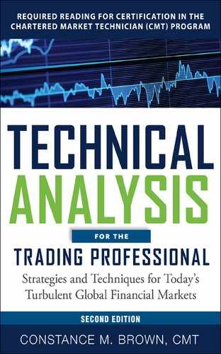
What do we even mean by a cycle? The Foundation for the Study of Cycles (foundationforthestudyofcycles.org) does not reference fixed periods in any definition describing a cycle. We obtain these assumptions from the programmers who code our market software. Cycle tools with fixed periods are easier to code and often the only tool offered in most analysis programs. Therefore most of us begin with these rudimentary tools in our hands. But at the same time the software vendor often limits our window of view to only ten years of historical data. We easily miss the fact that a cycle is a rhythmic fluctuation that repeats over time with reasonable regularity. It is not until the rhythm persists over a long span of time that we recognize this regularity cannot be the result of chance. No credible source will say cycles are impeccably precise, but some still believe the perfect fixed interval can be found. Assuredly, as soon as the “perfect” rhythmic period is identified, it will change its timing and even invert to become the market price high. We use cycles incorrectly. Rhythmic fluctuations can be more than just a fixed interval. The number series implying a spread progression of 8, 9, and 10 that repeats at 8 once again is also a cycle that has a repeatable rhythmic fluctuation. This is a cycle discovered by Samuel Benner which he published in 1876. Figure 2.0 is Benner’s Nine-Year Cycle in Pig-Iron Prices from 1834 to 1900. More follows about Benner shortly, but this particular cycle had a 44:1 win-to-loss ratio.

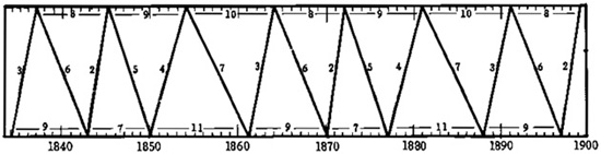
Figure 2.0 Benner 9Yr Cycle in Pig-Iron Prices 1834–1900
Source: Benner’s Prophecies, 1875

Consider the following example where the number of sunspots, along with other signs of solar magnetic activity, waxes and wanes on an 11-year cycle. We measure this cycle in glacial ice cores containing nitrate-rich layers that reconstruct a history of past events. These events, as measured by proton radiation, have a correlation to the number of sunspots and solar flares from the sun. Why do we care? The relentless churning of solar gases and the resulting solar storms make a difference to the earth’s magnetic field which scientists believe changes the yields of our agricultural produce. If we trade agricultural grains or financial markets, we should recognize the connection of food shortages leading to political instability and global trade disruptions.

Fixed period cycles fail to adjust to natural rhythms of expansion and contraction characteristics within markets. A growth-decay cycle means expansion and contraction attributes and those are easier to see in nature than in market swings. Just leave an orange out in the sun for a month and it is clear that contraction changes accompany decay. But many do not realize this occurs as well in markets on both the price axis, y axis, and x axis that defines time. The greater span of time one is studying, the harder it is to see the expansion and contraction aspects of the cycle. A 400-year chart of Gold may appear to display a fixed period cycle. But when a quarterly chart (three months within one bar) is expanded to detail the data in a daily presentation, the cycle timing that fits major price lows in the long horizon could be off significantly. Cycles offer us a tool to sharpen our awareness of the rhythmic undulations in a bigger picture and thereby help us to interpret the signals within our other technical methods. When this book was first written in 1997/1998 the illustrations and dialogue describing the charts of the Nikkei showed the conventional use of cycles. Read this section without changes so it can be used as a comparison of cycle convention versus the changes that followed after a decade of further trading experience and research.

Figure 2.1 is one of the most cyclically symmetrical markets in the world today: the monthly chart of the Japanese Nikkei Index. A 52- and 89-period cycle on the chart argues the case well that cycles are measurable, predictable, and for some markets exceptionally accurate. These two independent cycles also project extreme problems again for the Japanese market around the end of 2005 and the first quarter of 2006 when these two cycles bottom in a close juxtaposition. We know that cycles have a cumulative effect and multiple cycle lows that bottom in a close proximity of time will exacerbate the market decline into those projected market lows.

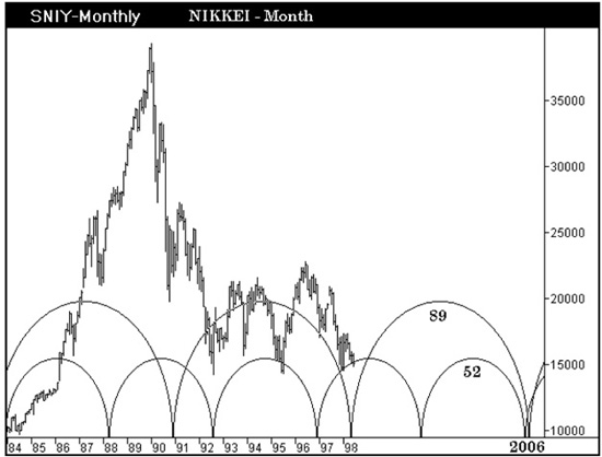
Figure 2.1 Nikkei 225 Index
Source: TradeStation. © TradeStation Technologies

While the monthly Nikkei Index displays the same 52-period cycle in Figures 2.1 and 2.2, the 89-period cycle has been replaced by an 85-period cycle in Figure 2.2. Both the 89- and 85-period cycles are anchored from lows just out of view to the left of the chart, which makes more recent market lows the third cycle bottoms for these cycle periods. The 85-period cycle accurately warned that a decline would unfold into January 1998. The 89-period cycle accurately warns of the decline unfolding now in June 1998. Traders who used the 85-period cycle were not wrong but would likely be confounded by this June decline if they thought that the Nikkei had established a bottom six months earlier. The 89-period cycle in conjunction with the 52-period warns that early 2006 will be a major problem for this market. By shifting the preference from the 89-period to that of an 85-period cycle, the forecast shifts back to 2005, and the character of the decline itself could be very different as the cycle lows are not as close together. An interpretation could be made that an orderly decline in 2005 would unfold in comparison to the sharp spike bottom implied by the 2006 cycles that bottom together in Figure 2.1. What is the correct period to use if both the nearby market interpretation and extended views can be changed so easily by just a minor period adjustment of 85 to 89 in these cycles? In reality, one period is not more correct than the other; we can see from these charts both had predictive value in 1998. However, both periods will be wrong if new price data are ignored and the periods defined today are not later adjusted for the markets’ natural growth and decay attributes that will develop between now and 2005.

Figure 2.2 Nikkei 225 Index
Source: TradeStation. © TradeStation Technologies, Inc.

In Figure 2.2 the major low that developed in July 1995 was missed altogether by the cycles using periods of 52, 85, and 89. We will address this particular low shortly, but let’s stick with growth-decay attributes within the markets for a moment. As soon as the phrase growth and decay is used, most traders will assume we are heading into a discussion about Fibonacci ratios. Let me offer the bottom line for this methodology up front: Fibonacci cycle projections will not provide us with the definitive answer when we ask, “What is the most important cycle within the market I trade now?” It is not good enough to tell a trader that both the 85- and 89-period cycles on a monthly chart are correct. We need something that will give us a higher probability than a six-month window of time from which to determine a major market bottom. While Fibonacci ratios alone will not provide us with the definitive answer, this mathematical series of numbers does offer an essential component in our quest to recognize what has immediate significance. The number series is certainly of value, but conceptually the Fibonacci sequence may have an even greater impact.

As a professional trader and student of the markets, one cannot escape an encounter with the remarkable Italian mathematician, Leonard of Pisa, better known as Leonardo Fibonacci. But did you know Fibonacci was not his name? That was a nickname, an abbreviation of “filius Bonacci.” If you are new to Fibonacci but can accept the bottom line of his theorem without the background discussion for proof, know that your financial livelihood will be very much tied to the ratios 0.146, 0.236, 0.382, 0.500, 0.618, 1.00, 1.618, and 2.618 and that they will directly impact your profit and loss.

Why? These ratios have been around for a very long time. Leonardo Fibonacci wrote about them in his book, Liber Abaci, in 1202, but the number sequence from which these ratios are derived was in use around 4700 BC when the Egyptians built the Great Pyramid of Gizeh. The slant edge of the Great Pyramid is almost exactly 0.618. To create the number series, add the first number to the second, the second to the third, and you develop the sequence: 1, 1, 2, 3, 5, 8, 13, 21, 34, 55, 89, 144, 233, 377, and so forth. These specific numbers will be of value to you as periods for moving averages and within indicators. The ratios themselves come from the fact that any given number over three in the series is approximately 0.618, or 61.8 percent, of the number that follows it. Any adjacent number in the sequence over five is approximately 1.618 times the number preceding it. Between alternate numbers, the higher will be approximately 2.618 times the first, and the lower number between alternates will be approximately 0.382.

The really interesting aspect about these ratios is that they are found in anything that has a growth and decay developmental cycle. Plants, animals, vegetables, minerals, and—you’ve guessed it—markets. As all living entities do exhibit these exact same expansion and contraction ratios, Leonardo’s mathematical theorem is viewed as a law of nature. It should not be surprising that these ratios are frequently respected within the markets. Markets expand and contract and so abide by the same law. If you want to know more, head to the Internet and start surfing. You will undoubtedly discover the original question concerning rabbit population growth and see that Leonardo Fibonacci and Darth Vader shared the same style of dress. But let’s move on to see how the Fibonacci number sequence applies to cycles in the markets.

In Figure 2.3 we are still viewing the Japanese Nikkei Index, but we have dropped down to a weekly chart. A symmetrical fixed-period cycle is charted that displays corresponding cycle bottoms at market lows near the end of 1993 and the start of 1997. The same chart also shows vertical broken lines that are numbered one through seven. The 1995 low marks the starting anchor for the vertical series of lines. Each vertical timeline plotted is derived from a Fibonacci ratio. These lines are called Fibonacci time cycles. At points 1 and 3 the line bisects a market low. Points 2, 4, 5, 6, and 7 all mark pivot points preceding a market pullback. That is the thing about Fibonacci time cycles that will be troubling for traders—not knowing if they are approaching a market high or low. True, a pivot implies a market trend reversal so assume a reversal from the present trend. But take a closer look at point 6. That is a significant Fibonacci cycle projection that denotes a market high. The Fibonacci cycle at point 6 immediately precedes a cycle low in the symmetrical cycle that accompanies the price bottom in early 1997. That just adds a lot of conflict. Which cycle method will be proved right? In hindsight the symmetrical cycle bottom was stronger, but the Fibonacci time cycle was also correct—it just did not amount to much of a trend reversal at point 6. The question of knowing what the magnitude or strength of a signal will be is the heart of the issue for a trader.

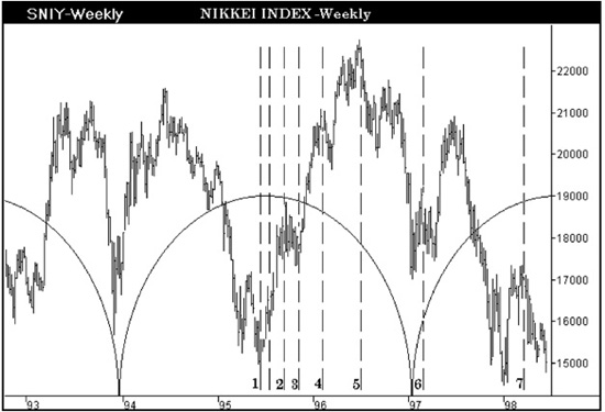
Figure 2.3 Nikkei 225 Index
Source: TradeStation. © TradeStation Technologies, Inc.

If we plot a second Fibonacci time cycle with the starting point at the market bottom near the close of 1993 (not on the chart), a Fibonacci time cycle from that low would not coincide with any other cycle marked in Figure 2.3. The additional information just becomes noise. Many of us have witnessed an in-depth Fibonacci time cycle analysis that failed. The work was not flawed—it was just that the firecracker, after having been ignited, did not produce any consequential reaction. All the right ingredients seemed to be present, but then nothing happened—a dud, or worse a reaction opposite to our expectations. Multiple Fibonacci cycles projected from numerous market lows reveal confluence points where different ratios overlap one another or form very tight cluster groups. The cumulative effect when cycles of varying periods or Fibonacci frequencies overlap to form a clustered group should mean a high-probability pivot and trend reversal for the market. While this is true for Fibonacci retracements derived from price, it is far less accurate for Fibonacci time projections.

The inaccuracies and weaknesses we all experience as traders with both symmetrical and Fibonacci cycle analysis may be caused by an oversight. This oversight is ignoring the basic premise that nothing is static; therefore, rescaling for cycles forming within multiple time horizons cannot be defined from linear or symmetrical periods. Figure 2.4 returns to the monthly bar chart for the Nikkei Index. The same two cycles displayed in Figure 2.2 are repeated in this chart showing 52 and 89 periods. In Figure 2.4, a 44-period cycle has now been added, and the heavier line helps locate the new period in this chart that captures the market low that was missed in January 1998. The 44-period cycle was selected as it also captures the price low that coincides at the cycle bottom marked at point 1. At point 2 both the 44- and 89-period cycles have a close proximity and contribute to the meltdown drop into the 1990 low. The cycle bottom at point 3 is late for the price low, but the same cycle period is also slightly early for the January 1998 bottom where three cycles are beginning to form a cluster now near point 4. We do not know which cycle period is most important, but clearly the market lows that coincide with the cycle bottoms clustering at point 4 are all significant. We still have the price low at point X that remains unidentified by any of the cycle periods selected up to this point. We will need to add one more cycle to capture this low.

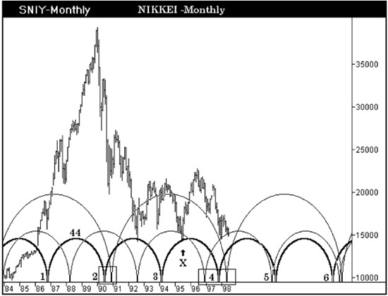
Figure 2.4 Nikkei 225 Index
Source: TradeStation. © TradeStation Technologies, Inc.

The cycle that is now highlighted by a heavier line in Figure 2.5 is a 56-period cycle. It marks the important low that occurred in 1995. We now have a chart with lots of cycles up to 1998 and nothing to suggest a low for another two years. In addition, the cycle with 56 periods on the heavier line marks the start of a rally in 1986. Will the future cycles be lows or mark continuations within established trends? That is an important observation many overlook as we condition ourselves to look for patterns that fit our assumptions and we then ignore information that may not fit our definitions. Figure 2.6 has all the cycles we have been building on in the prior charts. But now look at what happens when you use the Fibonacci cycle in a different way. Anchor the tight starting cluster of Fibonacci ratios between the two cycle bottoms plotted in 1986. Then let the Fibonacci series extend forward in time from this anchor point. You are not using a price low, but the symmetrical cycle bottoms clustered at the start of the chart, to project the Fibonacci cycles. Not only do the resulting Fibonacci cycles fall entirely on market lows but they are also lows of tremendous significance. Point 1 shows you the anchor point to start this projection. (A note added in 2011: Market prices at price swing extremes end the prior trend, but do not start the new trend. The new trend often begins with the first retracement that becomes a failure to resume the prior trend. Many technical tools give better accuracy when projected from the first retracement. There is more on this in the revised Chapter 4.) Point 2 is two periods late, but it is much earlier than the symmetrical cycle that is closest to it. Point 4 defines a major price low that is not even portrayed within our cycles plotted in this chart. Point 5 marks what promises to become the most significant of all the cycles preceding this cluster of numerous symmetrical cycle bottoms. As for point 6, it is the end of the tight cluster of cycles that will mark a capitulation bottom.

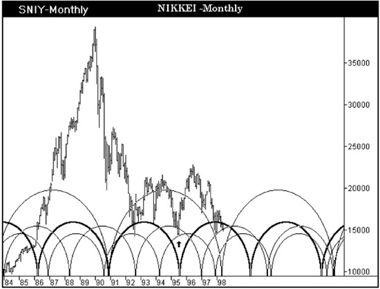
Figure 2.5 Nikkei 225 Index
Source: TradeStation. © TradeStation Technologies, Inc.

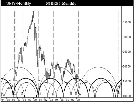
Figure 2.6 Nikkei 225 Index
Source: TradeStation. © TradeStation Technologies, Inc.

What have I learned since 1998? Was the next major cycle in Figure 2.6 a major bottom? No. The market had bottomed and basically frothed back and forth and the cycle marked the start of a strong rally. This is extremely important as markets can wait until a cycle has completed, but prices will be well off a price high or low. A cycle can mark where market acceleration will begin.

Two kinds of cycles were demonstrated: symmetrical and Fibonacci rhythms within the Nikkei Index. What I did not know then was that the method demonstrated was incorrect for the desired information sought.

Cycles have taught me that within the historical body of fixed cycle work there is brilliance and creativity that we have abandoned to our own detriment. Our thinking becomes very shallow when we hyperfocus on just the hunt for a trading signal. We forget that mastery of technical analysis is not the end goal, but only a collection of well-researched tools that we accumulate in an intellectual think box ready to be called upon to solve a problem. As experience matures it gets easier to recognize the tools needed for any given market puzzle developing.

There were three great cycle analyst masters who resided within the United States. They all used technical analysis to think about where we have been and used this information to see where their future could be heading. The first was Samuel Benner who wrote Benner’s Prophecies in 1875. This book was the first study with an extended forecast on market booms and panics in North America. Figure 2.8 is a chart from Benner’s book. His charts contained Fibonacci relationships that had never been documented before in his work.

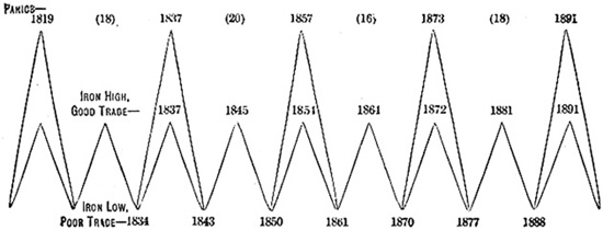
Figure 2.8 Pig-Iron Market Panics 1800–1991
Source: Benner Prophecies, 1875

The second master was brilliant in his study of fixed cycles: Edward R. Dewey, the founder and president of the Foundation for the Study of Cycles. This lifetime body of work is now in the safe keeping of the Market Technicians Association in New York (www.mta.org). Mr. Dewey’s brilliance was not just in the body of cyclical chart work that he developed, but in the diverse subjects he examined that we fail to consider today in our modern global markets. While his cycle work is important, it is his thought process that is even more valuable.

The third great master was William Delbert Gann. His lifetime work was the study of cycles on the horizontal, diagonal, and vertical axes of a market chart. His brilliance was in the utilization of geometry, harmonics, and astronomical time cycles. Simply put, Gann knew how to utilize geometric space in time. There are strong views for and against his work because most people writing books apply John Gann’s methods—the methods of the son not the father. W.D. Gann was a brilliant analyst because he could use his work to surmise social changes, outcomes of wars, and market movement. I will shortly show you a demonstration of this.

Consider some of the fixed period cycle work of Edward Dewey. Figure 2.7 is Mr. Dewey’s study of major real estate activity in the United States from 1795 to 1939. The description under the chart states, “Figure 8. Major Real Estate Activity. An index of real estate activity in the United States, 1795–1939, after adjustment for trend, compiled by Mr. Roy Wenzlick. An 18 year periodicity has been added by the author.” I then exaggerated Mr. Dewey’s cycle by making the line wider so it would reproduce more easily. This is an old hand-drawn chart, so please excuse the quality of the reproduction.

Figure 2.7 Major Real Estate Activity (U.S.A. 1795–1939)
Source: Cycles Classic Library Collection, Foundation for the Study of Cycles, 1987, Edward R. Dewey

When Mr. Dewey wrote “after adjustment for trend” he was telling us the data was detrended. A simple method of detrending is to create a one-period moving average and x-period average with a longer period. Subtract the value of the shorter period average from the longer and plot the result as a line. It becomes an oscillator as each time the one-period crosses the longer period it is a value of zero. When the shorter value is above the longer it will be a positive value and the value is negative when it is less than the longer period average. A real-time application will be found in Chapter 8 where a comparison is made between the RSI and this simple oscillator when it becomes more useful in strong trends.

Three great masters of cycle analysis have been named. How would these cycle gurus have fared in today’s markets?

To extend the Dewey real estate chart in Figure 2.7 to current times we need to find a common denominator. The interval of 18 years is 55 thirds (18 * 3 = 54 and add 1). Using 1938 from near the last cycle low (1938 * 3 = 5,814, add 110 (two cycles), then divide by 3 = 1974. This marks an interesting start of a tremendous DJIA bull market. If we add four cycles (220 thirds) to the year 1938, the cycle falls in the year 2011. But you may think that “the real estate crash came in 2008”. Good point, but that was the start of the crash, we are still in it, and we don’t have a bottom as this is written in March of 2011. You need to combine this cycle of Mr. Dewey’s with the Gann cycle discussed shortly. Mr. Dewey’s cycle work began with data from 1795 and remains valuable today to show where the inflection points are within the American business cycle.

Most of our vendors cut off our window of view after 10 years. It is difficult and expensive to purchase the historical data and then it often takes custom software to even see the data files in our procession. It is little wonder so few of us make the effort to connect the cycle work of our predecessors to current market data. The only way this will ever change is for you to communicate your needs to your vendor.

A soft real estate market means an economic downturn. Knowing this rhythm in real estate sharpens our awareness of the market risks. We knew a housing bubble was blooming with an eminent collapse as its resolution as that is historically how all bubbles burst. But we did not know as traders when the collapse would happen—or did we? As traders we do not establish a position based on this data, but we know and immediately recognize the significance of a trigger as it happens and can use our better trading tools with the early recognition that a major new trend is in force. Such analysis prepares us to act decisively when others around us are confused and emotional. We can act because we are prepared with a predetermined game plan in place.

Mr. Benner’s work came well before Mr. Dewey’s. Yet Benner also referenced real estate prices and commercial booms and panics in his Fibonacci cycle work of 1875. His book, Benner’s Prophecies of Future Ups and Downs in Prices is so rare and extremely expensive that I will reprint a portion of it before we continue our discussion. Please take special notice of the statements Benner wrote that I have highlighted in bold text.

Commercial Revulsions in this country, which are attended with financial panics, can be predicted with much certainty; and the prediction in this book, of a commercial revolution and financial crisis in 1891 is based upon the inevitable cycle which is ever true to the laws of trade, as affected and ruled by the operations of the laws of natural causes.

The panic of 1873 was a commercial revolution; our paper money was not based upon specie (specie refers to Gold and Silver), and banks only suspended currency payments for a time in this crisis.

In the Report of Finances for 1854 and 1855, it is stated that the adoption of the Federal Constitution in 1787 to the year 1798, no people enjoyed more happiness or prosperity than the people of the United States, nor did any country ever flourish more within that space of time. During all this time, and up to the year 1800, coin constituted the bulk of the circulation; after this year the banks came, and all things became changed, like the Upas tree, they have withered and impaired the healthful condition of the country, destroyed the credit and confidence which men had in one another.

The bank-note circulation began to exceed the total specie in the country in the years 1815, ’16, and ’17, and in the year 1818, the bank mania had reached its height; more than two hundred new banks were projected in various parts of the Union. The united issues of the United States Bank, and of the local banks, drove specie from the country in large quantities, and in the year 1819, when the culmination in general business had been reached, and contraction of the currency began to be felt, multitudes of banks and individuals were broken. The panic producing a disastrous revulsion in trade, caused the failure of nine-tenths of all the merchants in this country and others engaged in business, and spread ruin far and wide over the land.

Two-thirds of the real estate passed from the hands of the owners to their creditors.

A banker, in a letter to the Secretary of State, in 1830, describes the times as follows;

“The disasters of 1819 which seriously affected the circumstances, property, and industry of every district of the United States will be long recollected.

A sudden and pressing scarcity of money prevailed in the spring of 1822; numerous and very extensive failures took place in 1825; there was great revulsion among the banks and other monied institutions in 1826. The scarcity of money among the trades in 1827 was disastrous and alarming; 1828 was characterized by failures among the manufactures and trades in all branches of business.”

After the year 1828 business continued to be depressed, vibrating according to circumstances until 1834, a year of extreme dullness in all branches of trade; after which our stock of precious metals increased very fast, business revised, and in the year 1835 and ’36, the imports of gold and silver increased to an enormous extent; as the banks increased their reserves of species (gold and silver), they also correspondingly issued bank notes—each increased issue of paper money led to the establishment of new banks.

The State banks that had numbered in 1830 only three hundred and twenty-nine, with a capital of one hundred and ten millions, increased, according to the treasury report, by the first of January, 1837, to six hundred and twenty-four, or, including branches, to seven hundred and eighty-eight, with a capital paid in of two hundred and ninety millions.

Mark the result and culmination; a panic! In the month of May, 1837, a suspension of specie payments by all the banks, and a general commercial revulsion throughout the country, involving the fortunes of merchants, manufacturers, and all classes engaged in trade, in consequence of a ruinous fall in prices. This year of reaction makes the second year in our panic cycles, and is eighteen years from 1819.

History repeats itself with marvelous accuracy in detail from one panic year to another. The general direction of business after the panic of 1857 was on the same downward grade that had characterized the times after the panic of 1819 and 1837, until all business had culminated in depression in the year 1861, after which trade again improved, and was very active during the war of the rebellion and up to the year 1865, when a temporary reaction set in. Reader let me observe here, that if then had been the time for a commercial revulsion and panic in money, the catastrophe would have been the most deplorable national calamity upon record. However, the cycle was not then complete. And the commerce and trade of the country continued to be semi-prosperous until 1870, after which year commercial activity was the order of the day, all branches of business and manufacture flourished and was prosperous; our railroad building was astonishing in the world in the years 1871, ’72; but the end must come, and in September 1873, we had the culmination—a crashing panic, and reaction in all trades, manufactures, railroads, and industries, which is still going on, and we have not reached hard pan.

The panics of 1819, ’37, ’57, and ’73, during this period of years, stand out upon the pages of history of this country in their magnitude compared with other panics. Commencing with the commercial revulsion of 1819, we find it was eighteen years to the crisis of 1837, twenty years to the crisis of 1857; and sixteen years to the crisis of 1873—making the order of cycles sixteen, eighteen, and twenty years and repeat. The cycle of twenty years was completed in 1857, and the cycle of sixteen years ending in 1873, was the commencement of the repetition of the same order. It takes panics fifty-four years in their order to make a revolution, or to return in the same order; the present cycle consisting of eighteen years will end in 1891, when the next panic will burst upon us with all its train of woes.

So how did Benner do with his forecast for 1891? Allowing Benner plus or minus a year he did very well and hit the cycle low and high correctly in his book. That is why his book survived and entered numerous reprints. Figure 2.9 is the cycle he used to make his forecast. His book was the first of its kind.

Figure 2.9 Index of International Battles from 550–1957
Source: Cycles Classic Library Collection, Foundation for the Study of Cycles, 1987, Edward R. Dewey

In 1837, 1857, 1873, and 1893 a New York residential boom ended in a panic bust where housing prices collapsed. New York’s housing busts were caused by recessions (or “panics”) in the national economy recorded in the years of 1837, 1857, 1873, and 1892 to 1893. One of the ways we can research economic housing cycles is through newspaper advertising. Is having our current history recorded entirely by electronic means really the smartest thing for us to do? The New York Times has papers on file that were used to supplement historical data for these studies. In 1826 land that sold for $100 to $150 rose to $2,000, according to ex-New York Mayor Philip Hone. When banks failed and the economy fell into a depression, lots in the West 100s which cost $480 a piece in September 1836 were selling for $50 in April 1837.

The Great American Depression that followed the NYSE crash of 1929 to 1930 was not the worst depression in American history. Although we are taught as students that this was the worst period in American business history, Benner described the year 1819 as a period when nine-tenths of all businesses failed.

It is interesting that Benner stated that it takes 54 years from panic to panic, as Dewey also identified a 55-period quarterly cycle, or 18 years, that is, one-third of Benner’s cycle. If we take Benner’s forecast of 1891 as the start of a panic contraction period and add 54 years up to current times, the cycle falls on 1999. In hindsight we know a panic developed, but not a real estate panic one might try to associate with this cycle. The cycle mapping human sentiment was spot on and the 1999 to early 2000 top led to a panic that pushed the early Internet companies out of grace. Many fell from dot-coms to “dot gones.”

What we are learning in this example is how to use cycle analysis to give us a sense of where we stand today within an historical cycle of significance. That is far more valuable than the hunt for a single isolated entry point to establish a new trade. Do you want a fish, or do you want to know where the entire school of fish is hiding? That is why my first discussion of cycles missed the mark in 1996. Knowing where we are now in the context of a much bigger picture is invaluable. From these cycles we can ask important questions, such as, how did these events build into a major economic panic? Notice how Benner takes notice of the decline in reserves of gold and silver and the changes in public confidence concerning the valuation of paper currencies. Was this an ingredient that always contributed to the cycle panics of the past? I’ll leave you to answer that one as it is important to do the research. One easy way is to scan the papers from a year before a market bust sets in. The ads, the real estate listings and job offerings, the editorials, the news itself all paint a sentiment pattern that will show you there are similarities in human patterns that can be predictable.

I have a school in North Carolina that is dedicated to teaching advanced traders. One of the most important things I demonstrate is showing how a question or irregularity can become an opportunity to learn. Don’t run away from the unknown. Whatever the trader brings to the school, regardless of culture or technique, I will turn their technique into a puzzle they had never considered before so they have to think in ways that will increase their probability of being right. Most people shrug their shoulders and state that they don’t know the answer. The best traders recognize the opportunity and want to run into the unknown to better their understanding. Their worst response is to take someone else’s answer and assume that it is correct when they don’t really get it themselves.

The concerns for a diminishing confidence in our currency form a cycle of consumer sentiment that Dewey and Benner both warned us about. Their chart work should make us think about the risk blooming in current times. We also need to ask, “what contributed to the recovery after a major business cycle contraction?” Both state and show that manufacturing was the key. It remains so today. That means education is key in America as we have to make products no one else can make. The race is on. But the manufacturing industry for any country is tied to the ability to sell its goods elsewhere and that means you need an opinion on currencies. Too many stock traders believe they need not spend time on analyzing currencies. But if you analyze the gold stocks GFI and NEM and find they have a slight out-of-step correlation, you better realize that GFI is based on a revenue stream in South African Rand currency. You are a currency trader whether you want to be or not. This is not about an analyst becoming a fundamentalist. It is only showing you that we must think about what we are seeing in our charts, indicators, cycle work, and intermarket relationships in order to do exceptionally well in this global environment.

Should we not be asking ourselves, “how often has the world seen a war break out after a financial collapse?” Is there a relationship in timing between the collapse and political instability? Was it a loss of confidence in currency that triggered the wars, a drastic change in the cost and availability of food that led to political instability, or debt that could not be sustained due to more benefactors than worker bees paying into the social programs? Whatever the ultimate triggers, asking ourselves questions helps us to focus on a broader range of markets that provide us with balance that will increase the probability of our work. Looking how cycles fall within the Nikkei price data is superficial if the discussion goes no deeper.

Consider further the work of Dewey. Figure 2.9 shows Dewey’s study of an Index of International Battles from 550 through 1957. The cycle interval is 10.8 years. We know the half cycle for sunspot and solar storm activity is 11 years. Agricultural yields are also tied to an 11-year cycle. Is one of the factors influencing weather patterns the changes in the earth’s magnetic field which has a similar cycle? Finding if one set of data influences another set of data requires a statistical study. But first you need to have the data and lots of it.

Figure 2.10 is Dewey’s long-term chart for European Wheat prices from 1500 to 1869. This data was collected by Lord Beveridge who discovered there was a 54-year cycle in Wheat prices. It is interesting how this cycle period keeps reappearing in this discussion.

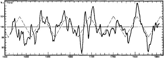
Figure 2.10 European Wheat Prices 1500–1869
Source: Cycles Classic Library Collection, Foundation for the Study of Cycles, 1987, Edward R. Dewey

Dewey studied cycles that mapped human sentiment and activity in ingenious ways. He thought outside the box of convention. This is part of the brilliance of his work and what we can easily miss in our own work today if we only focus on a trading signal within a single market. If we stop thinking about why we are studying a cycle, we easily forget that the real purpose is to increase our probability within a complex multitiered global environment. Trade signals do not occur in isolation any more.

In Figure 2.11 we see Dewey’s 9-year cycle in new Presbyterian church members in the United States from 1826 through 1948. Was Dewey studying the growth of the Presbyterian church? No. In economic times of hardship church membership increases; in easier times membership declines. Dewey was not the only one to study economic cycles through various habits and trends within the general public.

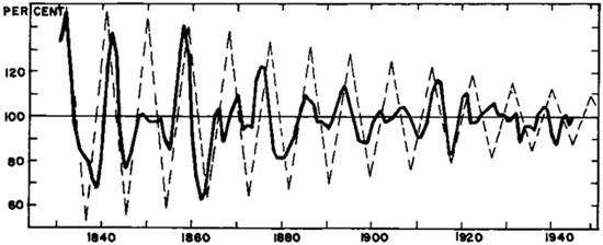
Figure 2.11 Growth of the Presbyterian Church in America (1826–1948)
Source: Cycles Classic Library Collection, Foundation for the Study of Cycles, 1987, Edward R. Dewey

The third cycle analyst from the United States is perhaps the least understood. Few students of Gann’s work realize that the first edition of his book, How to Make Profits Trading in Commodities (W.D. Gann & Son, Inc., 1941), describes different charts from those in his revised 1951 edition (Lambert-Gann Publishing Company, Inc.) in distribution today. There are so few copies of the 1941 edition that they are hand corrected. In addition, the 1941 release was a more open and unveiled dialogue that I suspect was due to concerns about the growing war in Europe.

Gann wrote a segment on page 310 titled “Why Hitler Will Lose the War”. Keep in mind that this student of markets was making a forecast before the Japanese attack on Pearl Harbor caused the United States to enter World War II. His views on why wars are fought remain true today. While Gann was a technician of markets, he used this knowledge to develop a theory of the bigger picture in which he must trade and live. Gann wrote:

Before going into the details of why Hitler will lose the war, it is important to analyze for what the war is being fought. We read much about the fight against Nazism, Communism and Socialism, and that the war is being fought to preserve democracy and the freedom of the seas. This is not a true picture or a true fact of what the war is being waged over, but when the war is over and the smoke clears away, the world and the public will know for what the war was fought.

This war is no different than any other war. It is being fought for commercial supremacy to determine WHO is to dominate the commerce of the world in the future. Germany wants to dictate prices and dominate the commerce of the world, and England wishes to do the same. Russia would like also to do the same thing.

It now appears that the New Dealers in the United States would like to dictate everything to the world. England has always fought to maintain freedom of the seas and control the commerce of the world, and England knows that it is a part of wisdom to work with the United States, and with Russia to determine the trade relations after the war is over. Germany will lose the War because they do not have control of the sea. As long as the United States and England dominate the seas they will rule the trade of the world.

Comparing TIME PERIODS of the past, Hitler’s campaign into Russia has not made the progress that Napoleon made in the same number of days. Hitler has every improved machine for waging war and moving rapidly. Yet the big Blitzkreig has failed to keep up with the pace of Napoleon with his horses and mules. Something is wrong! It is this writer’s opinion that Hitler’s “Waterloo” was written the day he made the advance into Russia. No chain is stronger than its weakest link. No man has ever been so smart that there isn’t another smarter. The other nations fighting against Hitler will find the weak point, and that weak point will be the undoing of Hitler, and Germany will lose the war.

Gann’s 1941 release of How to Make Profits in Commodities occurred before any of these statements about the war, which showed the strength of his research techniques, had been proven true. In his 1952 edition, in circulation today, Gann removed not only the commentary with his opinion on the war, but he changed some of the chart references. Why? Gann wanted us to see he could prove the exact same cycles applied a decade later when he revised the first edition.

The more I study cycles of fixed periods the clearer it becomes to me that they are of greatest value in the longer term. Human events are difficult to recognize in shorter cycles. Longer cycles make traders or analysts far more aware and knowledgeable about the trading environment in which they are operating.

Did I find a solution to the problems inherent to all fixed period cycles demonstrated in my first edition? Is there a better approach to timing market entry, exits, and can we be warned when a market will form a pattern of distribution and go nowhere? Yes, there are better tools for trading and we can be warned when to stay away from a market. This alone is invaluable for risk assessment.

In my opinion the work of W.D. Gann has provided a better solution to the problem of timing trades, but his work is of particular value in the longer term as well. Both Benner and Dewey called some of our current market strife, but how would Gann have fared with calling today’s market turmoil?

Gann devoted a tremendous amount of time to what he described as the 56-year cycle, or the “Great Cycle,” because it is based on 144. Gann describes the importance of the Square of Twelve (144) in Gann’s writings, Mathematical Formula for Market Predictions: The Master Mathematical Price, Time, and Trend Calculator. The Great Cycle will be discussed further in Chapter 9 when we have had a chance to look at Gann’s Wheel to extract price and time targets. But first you will want a credible example of his analysis techniques applied in recent markets.

Gann’s approach to market timing can be found in the book edited by David Keller, “Breakthroughs in Technical Analysis: New Thinking from the World’s Top Minds” (Bloomberg Press). I was asked to write Chapter 5. It was written in 2006 and the book was released in early 2007. On page 104 you will find the following, “Gann’s methods warn that the years 2008 to 2012 will be difficult ones.” I tried to warn readers in this book, as this was a horrific cycle approaching on the horizon. So far Gann’s cycle has performed in current markets very well. This particular cycle of Gann’s was correlated to times of great turmoil with wars, business and bank failures, political unrest, and food panics stretching across 100 years of history. As a trader it does not bother me that I don’t know why something will happen. Just give me the when and suddenly all the other technical methods I use seem to become far more effective and easier to interpret.

But if 2008 to 2012 were foretold to be rough years and we are still living through them now, can Gann analysis warn us when the next bear market will unravel global markets again? Yes. The same cycle and confluence of supporting cycles point to 2019 to 2021.

However, knowing a target date doesn’t end the research. To begin with, one must accept from Gann’s cycle warning of 2008 to 2012 that this bear market is not over. Therefore, we need to think whether the two dates are connected. Is one market leading all the others? If there is a market leader do we focus on the timing of that market, such as China, or do we focus on our own markets?

Gann’s time analysis utilizes cycles borrowed from natural law and the laws of vibration. There is a pile of hoopla out there on this subject that is not worthy of print. What people fail to recognize is that books written in the late 1800s and early 1900s used the term natural law to describe the movement of planets. It was the study of natural law or, in today’s language, the study of astronomy. If you are a beginner, focus on astronomy (the science), and stay away from astrology. Eventually you will start to make connections that will lead you to study mundane astrology. But even this is mathematically different from what is used to prepare a newspaper column with daily horoscopes or write an emotionally charged newsletter that the sky is falling; sell all. What you are likely thinking about is natal astrology when you read the phrase ‘natural law’ and I haven’t any interest in natal astrology either. The data from the NASA website can be examined by chi-square tests and more. I want mathematical proof before risking my own bank account and likely you do too.

The truth is, even the 54-year cycle can disappear as it did in 1960. Fixed cycle enthusiasts will describe the beat of a cycle as the cumulative sum of numerous cycles all working to enhance or diminish the strength of a cycle beat. But when a strong cycle reappears, this description does not answer why the period begins with an offset interval from when it was last seen. The answer is that nature does not depend on fixed cycles.

Gann was a master of finding confluence targets on all three axes. He worked to identify objectives on the horizontal (price), diagonal (geometry), and vertical (time) axes. If you understand the concept of a confluence target zone on the horizontal price axis, it is easier to grasp the concept of confluence time targets along the vertical axis.

The concept of confluence price target zones will be discussed in Chapter 6 and is the focus of my book, Fibonacci Analysis (Bloomberg Press). Confluence price targets are narrow price ranges where different Fibonacci ratios cluster tightly together. They must be different Fibonacci ratios derived from several different price ranges. These target zones do not form a grid on the horizontal axis with a fixed interval between each target zone. The separation or spread between targets is irregular because markets expand and contract. The truth is that this is also found along the time axis as well and the changing intervals between cycle beats can be explained by natural law sciences.

Figure 2.12 shows the China Shanghai Composite with preliminary testing to develop cycles for time analysis. Gann states the following in one of his early works, Truth of the Stock Tape (1923, p. 116): “The most important thing of all is the Time factor, which I use in making up my annual forecasts.” In Gann’s book, Tunnel Through the Air, he states through his fictitious character Robert, “I have determined the major and minor time factors which repeat in the history of nations, men and markets” (p. 70).

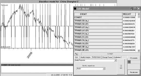
Figure 2.12 China Shanghai Composite with Time Analysis Study, Aerodynamic Investments Inc., © 1996–2011, Daily Market Report, www.aeroinvest.com
Source: Market Trader Gold, Alphee Lavoie and Sergey Tarasov

The specific event being tested in Figure 2.12 is called a retrograde cycle. We will take an introductory look at a few of Gann’s methods in Chapter 9.

While Benner, Dewey, and Gann all had different ways of charting cycles and focused on some that at first appear similar, they had in common something even more valuable; they were thinkers. These men used their cycle work to forecast and time the sentiment changes that impact on their business environment based on the rhythmic patterns of the past.

Endnotes

Dewy, E.R., with Mandino, O., Foundation of the Study of Cycles, New York: Hawthorn Books, Inc., 1971.