
CHAPTER
THREE
BOND MARKET INDEXES
Bernard J. Hank Professor of Finance
University of Notre Dame
DAVID J. WRIGHT, PH.D.
Professor of Finance
University of Wisconsin–Parkside
The value of nonmunicipal bonds outstanding in the United States at over $8 trillion is fairly close to the combined value of equity in the United States, and a similar comparison holds for world capital markets, where the value of fixed income securities is typically similar to the total value of equity. The only instance where this capital comparison does not hold is in some emerging-market countries, where the bond markets have not yet developed. Given the economic importance of fixed income markets, it is difficult to understand why there has not been greater concern and analysis of bond market indexes. Part of the reason for this lack of analysis of bond market indexes is the relatively short history of these indexes. Specifically, in contrast to stock market indexes that have been in existence for over 100 years, total rate-of-return bond indexes were not developed until the 1970s, and those created in the 1970s were limited to U.S. investment-grade bonds. For example, indexes for U.S. high-yield bonds, where the market has grown to over $1 trillion, were not established until the mid-1980s, which is also when international government bond indexes were created.
There are four parts to this chapter. The first section considers the major uses for bond market indexes. The second section is concerned with the difficulty of building and maintaining a bond market index compared with the requirements for a stock market index. The third section contains a description of the indexes available in three major categories. Finally, we present the risk/return characteristics of the alternative bond market sectors and examine the correlations among the alternative indexes.
USES OF BOND INDEXES
An analysis of bond market indexes is important and timely for several reasons. First, the bond portfolios of both pension funds and individuals have grown substantially in recent years; sales of fixed income mutual funds have exceeded equity mutual fund sales in a number of years. With the increase in the number and size of bond portfolios, investors and portfolio managers increasingly have come to rely on bond indexes as benchmarks for measuring performance and, in the case of those managing portfolios on a performance-fee basis, for determining compensation. There are numerous indexes of differing construction that purport to measure the aggregate bond market and the major sectors of the market (government, corporate, and mortgages). An obvious concern is the choice of an appropriate index that will provide an accurate benchmark of bond market behavior.
Second, benchmarks for bond index funds have become increasingly popular because those who monitor the performance of bond portfolios have discovered that, similar to equity managers, most bond portfolio managers have not been able to outperform the aggregate bond market. The amount of money invested in bond index funds grew from $3 billion in 1984 to over $400 billion in 2010. Given the total size and growth of the bond market, it is estimated that bond index funds could grow to over $600 billion during the second decade of the twenty-first century.
The behavior of a particular bond index is critical to fixed income managers who attempt to replicate its performance in an index fund. Clearly, if all indexes move together, one would be indifferent to the choice of a particular index. We examine the return correlations between the various indexes and their risk/return characteristics. The analysis of long-term risk/return and correlations is important because index numbers may differ markedly over short periods of time and yet still exhibit similar long-run movements.
Portfolio managers of a bond index fund need to rebalance their assets to replicate the composition, maturity, and duration of the bond market. As shown in Reilly, Kao, and Wright,1 the composition of the bond market changed dramatically during the 1980s, and there have been continuing changes during the 1990s and early 2000s. It is possible to use the indexes to document the intertemporal changes in the makeup, maturity, and duration of the bond market that have influenced its risk and return characteristics.
Third, because of the size and importance of the bond market, there has been and will continue to be substantial fixed income research; the bond market indexes can provide accurate and timely measurement of the risk/return characteristics of these assets and the characteristics of the market, as noted earlier. For example, the time-series properties of equity index returns have been examined extensively, but these same tests were not applied to bond market returns. Our investigation indicated significant autocorrelation in bond market index returns, which were explained by examining the intertemporal behavior of U.S. Treasury securities with different maturities.2
BUILDING AND MAINTAINING A BOND INDEX
To construct a stock market index, you have to select a sample of stocks, decide how to weight each component, and select a computational method. Once you have done this, adjustment for stock splits typically is automatic, and the pricing of the securities is fairly easy because most of the sample stocks are listed on a major stock exchange or actively traded in the over-the-counter (OTC) market. Mergers or significant changes in the performance of the firms in an index may necessitate a change in the index components. Other than such events, a stock could continue in an index for decades. (On average, the Dow Jones Industrial Average has about one change per year.)
In contrast, the creation, computation, and maintenance of a bond market index is more difficult for several reasons. First, the universe of bonds is broader and more diverse than that of stocks. It includes U.S. Treasury issues, agency series, municipal bonds, and a wide variety of corporate bonds spanning several segments (industrials, utilities, financials) and ranging from high-quality, AAA-rated bonds to bonds in default. Furthermore, within each group, issues differ by coupon and maturity, as well as by sinking funds and call features. As a result of this diversity, an aggregate bond market series can be subdivided into numerous subindexes; the Bank of America Merrill Lynch series (B of A-ML), for example, contains over 150 subindexes.
Second, the universe of bonds changes constantly. A firm typically will have one common stock issue outstanding, which may vary in size over time as the result of additional share sales or repurchases. In contrast, a major corporation will have several bond issues outstanding at any point in time, and the characteristics of the issues will change constantly because of maturities, sinking funds, and call features. This constant fluctuation in the universe of bonds outstanding also makes it more difficult to determine the market value of bonds outstanding, which is a necessary input when computing market-value-weighted rates of return.
Third, the volatility of bond prices varies across issues and over time. As indicated in Chapter 7, bond price volatility is influenced by the duration and convexity of the bond. These factors change constantly because they are affected by the maturity, coupon, market yield, and call features of the bond. Also, market yields have become more volatile, which, in turn, has an effect on the value of embedded call options and makes it more difficult to estimate the duration, convexity, and implied volatility of an individual bond issue or an aggregate bond series.
Finally, there can be significant problems in the pricing of individual bond issues. Individual bond issues generally are not as liquid as stocks. While most stock issues are listed on exchanges or traded on an active OTC market with an electronic quotation system (NASDAQ), most bonds (especially corporates) have historically been traded on a fragmented OTC market. Notably, this problem will be alleviated in the future with expanded trading on electronic platforms.3
DESCRIPTION OF ALTERNATIVE BOND INDEXES
This section contains three subsections to reflect three major sectors of the global bond market: (1) U.S. investment-grade bonds (including Treasury bonds), (2) U.S. high-yield bonds, and (3) international government bonds. We examine the overall constraints and computational procedures employed for the indexes in these three sectors.
Several characteristics are critical in judging or comparing bond indexes. First is the sample of securities, including the number of bonds as well as specific requirements for including the bonds in the sample, such as maturity and size of issue. It is also important to know what issues have been excluded from the index. Second is the weighting of returns for individual issues. Specifically, are the returns market-value weighted or equally weighted? Third, users of indexes need to consider the quality of the price data used in the computation. Are the bond prices used to compute rates of return based on actual market transactions, as they almost always are for stock indexes? Alternatively, are the prices provided by bond traders based on recent actual transactions or are they the traders’ current “best estimate”? Finally, are they based on matrix pricing, which involves a computer model that estimates a price using current and historical relationships? Fourth, what reinvestment assumption does the rate of return calculation use for interim cash-flows?
U.S. Investment-Grade Bond Indexes
Four firms publish ongoing rate-of-return investment-grade bond market indexes. Three of them publish a comprehensive set of indexes that span the universe of U.S. bonds: Barclays Capital (BC) (formerly Lehman Brothers), Bank of America-Merrill Lynch (B of A-ML), and Morgan Stanley Smith Barney (MSSB). The fourth firm, Ryan Labs (RL), concentrates on a long series for the Treasury bond sector.
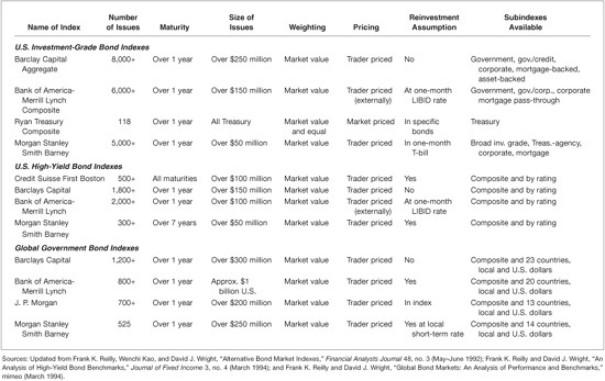
Exhibit 3–1 summarizes the major characteristics of the indexes created and maintained by these firms. Three of the four firms (BC, B of A-ML, and MSSB) include numerous bonds (over 5,000), and there is substantial diversity in a sample that can include Treasuries, corporates (credits), mortgage-backed, and asset-backed securities. In contrast, the RL series is limited to Treasury bonds and has a sample size that has varied over time based on the Treasury issues outstanding (i.e., from 26 to 118 issues). All the indexes require bonds to have maturities of at least one year. The required minimum size of an issue varies from $50 million (MSSB) to $200 million (BC), whereas the Treasury issues used by RL are substantially larger. All the series include only investment-grade bonds (rated BBB or better) and exclude convertible bonds and floating-rate bonds. The three broad-based indexes by BC, B of A-ML, and MSSB also exclude government flower bonds, whereas RL has included these bonds in its index because flower bonds were a significant factor in the government bond market during the 1950s.
EXHIBIT 3–1
Summary of Bond Market Indexes
The two major alternatives for weighting are relative market value of the issues outstanding and equal weighting (also referred to as unweighted). The justification for market-value weighting is that it reflects the relative economic importance of the issue and is a logical weighting for an investor with no preferences regarding asset allocation. Although this theoretical argument is reasonable, it is important to recognize that in the real world it is difficult to keep track of the outstanding bonds, given the possibility of calls, sinking funds, and redemptions. The alternative of equal weighting is reasonable for an investor who has no prior assumptions regarding the relative importance of individual issues. Also, equal weighting is consistent if one is assuming the random selection of issues. Finally, an equally weighted index is easier to compute, and the results are unambiguous because it is not necessary to worry about outstanding market value owing to calls and so on. The three large-sample indexes are value-weighted, whereas RL has created both a value-weighted and an equal-weighted series (for comparability, we use the value-weighted series).
As noted, one of the major problems with computing returns for a bond index is that continuous transaction prices are not available for most bonds. RL can get recent transaction prices for its Treasury issues, whereas MSSB gets all prices from its traders. As noted, these trader prices may be based on a recent actual transaction, the trader’s current bid price, or what the trader would bid if he made a market in the bond. Both BC and B of A-ML use a combination of trader pricing (B of A-ML from an external source) and matrix prices based on a computer model. Because most of the individual issues are priced by traders, the majority of each index is based on trader prices.
The indexes also treat interim cash-flows differently. RL assumes that cash-flows are immediately reinvested in the bonds that generated the cash-flows, MSSB assumes that flows are reinvested at the one-month T-bill rate, B of A-ML assumes reinvestment at the one-month London interbank bid (LIBID) rate, whereas BC does not assume any reinvestment of funds. Obviously, immediate reinvestment in the same bond is the most aggressive assumption, whereas no reinvestment is the most conservative.
U.S. High-Yield Bond Indexes
There are two notable points about high-yield (HY) bond indexes. First, they have a shorter history than the investment-grade bond indexes. This is not surprising because, as shown in several studies, this market only became a recognizable factor in 1977, and its major growth began in about 1982.4 Therefore, the fact that HY bond indexes began in about 1984 is reasonable.
Second, earlier we noted the general difficulty of creating and maintaining bond indexes because of the constant changes in the size and characteristics of the sample and the significant pricing problems. The fact is that these difficulties are magnified when dealing with the HY bond market because it experiences more extensive sample changes owing to defaults and more frequent redemptions. In addition, the illiquidity and bond pricing problems in the HY bond market are a quantum leap above those faced in the government and investment-grade corporate bond markets.
As shown in Exhibit 3–1, four investment firms have created HY bond indexes Credit Suisse First Boston (CSFB), Barclays Capital (BC), Bank of America-Merrill Lynch (B of A-ML), and Morgan Stanley Smith Barney (MSSB). The investment firms also have created indexes for rating categories within the HY bond universe: BB, B, and CCC bonds.
The summary of characteristics in Exhibit 3–1 indicates that there are substantial differences among the HY bond indexes. This contrasts with relatively small differences in the characteristics of investment-grade bond indexes. The number of issues in the alternative HY bond indexes varies from about 300 HY bonds in the MSSB series to 1,900 bonds in the B of A-ML series. Some of the differences in sample size can be traced to the maturity constraints of the particular index. The large number of bonds in the B of A-ML series can be explained in part by its maturity guideline, which includes all HY bonds with a maturity over one year compared with a seven-year maturity requirement for the MSSB series.
The minimum issue size is also important because MSSB has a minimum issue size requirement of $50 million compared with $100 million (CSFB and B of A-ML) and $150 million (BC).
Notably, there are significant differences in how the alternative indexes handle defaulted issues. The treatment varies, from dropping issues the day they default (B of A-ML) to retaining them for an unlimited period subject to size and other constraints (CSFB and BC). In contrast, there is no difference in return weighting; that is, all the indexes use market-value weighting.
All the bonds in the HY bond indexes are trader priced except for B of A-ML, which uses matrix pricing for a few of its illiquid issues. The difficulty with trader pricing is that when bond issues do not trade, the price provided is a trader’s best estimate of what the price “should be.” Matrix pricing is likewise a problem because each issue has unique characteristics that may not be considered by the computer program. Therefore, it is possible to get significantly different prices from alternative traders or matrix pricing programs.
All the indexes except BC assume the reinvestment of interim cash-flows, but at different rates—that is, the individual bond rate, the one-month LIBID rate, or a T-bill rate. Finally, the average maturity and the duration for the indexes are consistent with the constraints on the index: CSFB, BC, and B of A-ML have one-year minimums and lower durations, whereas MSSB with a seven-year minimum is at the high end.
In summary, there are significant differences in the characteristics of the alternative HY bond indexes in terms of the samples and pricing. One would expect these differences to have a significant impact on the risk/return performance and the correlations among indexes.5
Global Government Bond Market Indexes
Similar to the HY bond indexes, these global-based indexes are relatively new (beginning in 1985) because there was limited interest in these markets prior to the 1980s. The summary description in Exhibit 3–1 indicates numerous similarities among the indexes by the four investment firms (J. P. Morgan [JPM], Barclays Capital [BC], Bank of America-Merrill Lynch [B of A-ML], and Morgan Stanley Smith Barney [MSSB]). An exception is the minimum size, which varies from $200 million (JPM) to $1 billion (B of A-ML). In turn, this issue-size constraint has an impact on the sample sizes, which ranges from JPM at 500 to BC with over 800 bonds. The indexes are the same regarding market value weighting and trader pricing. All of them except BC assume the reinvestment of cash-flows with small differences in the reinvested security. The final difference is the number of countries included, which varies from 13 (JPM) to 23 (BC).
RISK/RETURN CHARACTERISTICS
The presentation of the risk/return results is divided into two subsections. The first subsection presents and discusses the results for the U.S. indexes, including government and investment-grade bonds, as well as HY bonds. The second subsection provides a similar presentation for global bond indexes, including both domestic and U.S. dollar returns.
U.S. Investment-Grade and HY Bonds
The arithmetic and geometric average annual rates of return and risk measures are contained in Exhibit 3–2 for the period beginning in 1986, when the data are available for almost all the series except the Altman defaulted bond series, which began in 1987. We show the BC index for U.S. investment-grade bonds because it has been shown that all the investment-grade bond series are very highly correlated.6
EXHIBIT 3–2
Rates of Return, Risk, and Annual Range for U.S. and Global Bond Indexes (1986–2010)
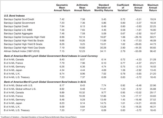
When viewing the results in Exhibit 3–2 and Exhibit 3–3, one is struck by two factors. The first is the generally high level of mean returns over this 25-year period, wherein the investment-grade bonds experienced average annual returns of between 7% and 8% and the HY bonds attained returns between 7% and almost 10%.
EXHIBIT 3–3
Geometric Mean Return versus the Standard Deviation of U.S. Bond Index Returns (1986–2010)
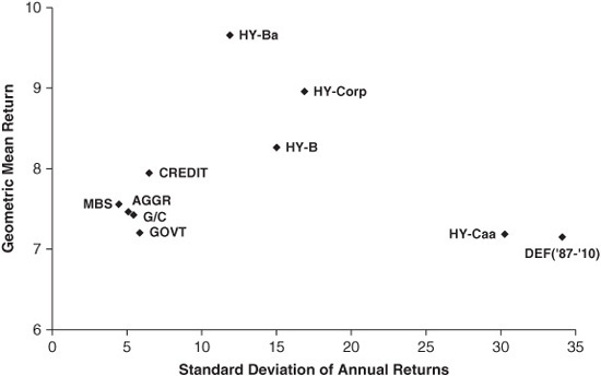
The second observation is that the relationship between return and risk (measured as the standard deviation of annual returns) generally was consistent with expectations. The investment-grade bond indexes typically had lower returns and risk, whereas the HY bond indexes had higher returns and risk measures. The major deviations were the high-risk segments (Caa-rated bonds and defaulted bonds), which experienced returns clearly below HY debt but risk substantially above all other assets.7 The Ba-rated bonds experienced abnormally positive results because they experienced returns clearly above other HY bonds but experienced the lowest risk among any other HY bond sector.
Global Government Bonds
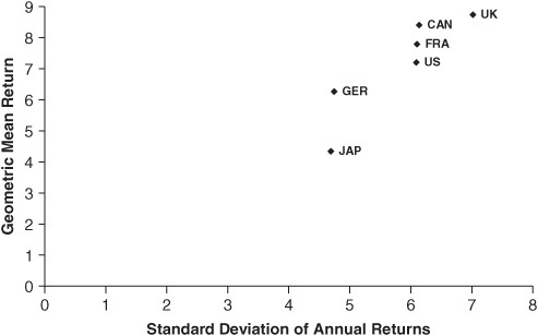
These results will be considered in two parts, involving results in local currency and in U.S. dollars. The results in Exhibits 3–2 and 3–4 show significant consistency between the risk and returns in local currency. Within Europe, Germany experienced the lowest return (6.26%), while the United Kingdom had the highest return (8.74%) but also experienced the highest risk (over 7% for the United Kingdom versus less than 5% for Germany). The only country that deviated from the main security market line was Japan, which experienced low risk but very low return (about 4.3%).
EXHIBIT 3–4
Geometric Mean Return versus the Standard Deviation of Country Government Bond Index Returns in Local Currency (1986–2010)
The return/risk results in U.S. dollars are shown in Exhibits 3–2 and 3–5. The graph in Exhibit 3–5 makes it clear that the results change substantially with the conversion to U.S. dollars. Specifically, the United States is clearly the low risk/return market, in contrast to Canada that had the highest return and the lowest risk except for the United States. France, the United Kingdom, and Germany had similar risk but France experienced the highest return followed by the UK and then Germany. Japan was below the consensus line with the highest risk and returns below all countries but the United States.
EXHIBIT 3–5
Geometric Mean Return versus the Standard Deviation of Global and Country Government Bond Index Returns in U.S. Dollars (1986–2010)
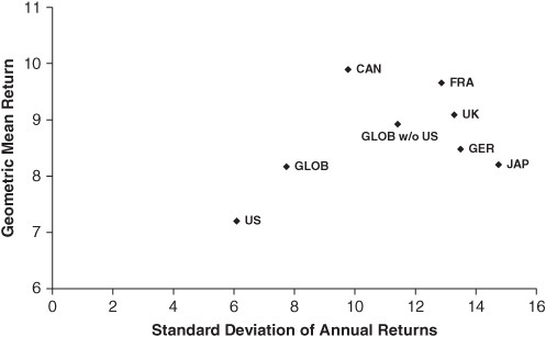
In addition to the individual countries, there is a global index with and without the United States. Both these indexes were consistent with overall results.
CORRELATION RELATIONSHIPS
The correlations likewise are presented in two parts: U.S. bond market results and global bond market results.
U.S. Investment-Grade and HY Bonds
The correlation results in Exhibit 3–6 confirm some expectations about relationships among sectors of the bond market but also provide some unique results. The expected relationships are those among the five investment-grade bond indexes. Because all these are investment grade, there is a small probability of default, so the major factor influencing returns is aggregate interest-rate changes based on the Treasury yield-curve. Therefore, since these index returns have a common determinant (Treasury bond rate changes), they are very highly correlated. Specifically, the correlations among the BC investment grade indexes range from about 0.79 to 0.99, with the results for the mortgage bond sector at the low end because of the impact of embedded call options on mortgage bonds.
EXHIBIT 3–6
Correlation Coefficients of the U.S. Bond Index Monthly Returns (1986–2010)

The HY bond results show two distinct patterns. First, the correlations among the HY indexes are quite high, ranging from 0.72 to 0.96. In contrast, the correlations among investment-grade bonds and HY bonds have a greater range and are significantly lower, generally ranging from about 0.00 to 0.56. Not surprisingly, the highest correlations are between Ba-rated bonds and investment-grade bonds, whereas the lowest correlations (typically insignificant) are between investment-grade bonds and Caa-rated bonds.
The correlations of defaulted debt with other segments were diverse but not unexpected. The correlations between defaulted debt and investment-grade debt generally were negative and sometimes significant. In contrast, the correlations among defaulted debt and various HY bonds were relatively large positive values, and all were significant.
Global Government Bond Correlations
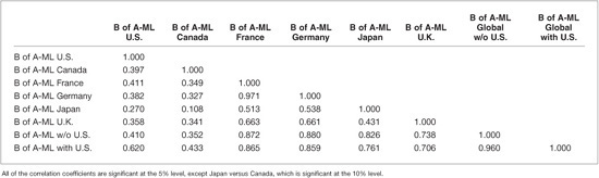
Again the discussion is in two parts, wherein we consider the local currency results and then U.S. dollar results. Exhibit 3–7 contains correlations among returns in local currencies. The correlations of Canada with all European countries indicate a similar relationship (about 0.50), with Japan at 0.33, and the U.S.–Canada correlation was about 0.75. In turn, France had a strong correlation with Germany (0.85)—its major trading partner in Europe—and 0.68 with the United Kingdom. Japan had correlations with the European countries between 0.31 and 0.37 and a correlation with the United States of only 0.34, even though Japan and the United States conduct significant trade.
EXHIBIT 3–7
Correlation Coefficients of the U.S. Bond Index Monthly Returns (1986–2010)
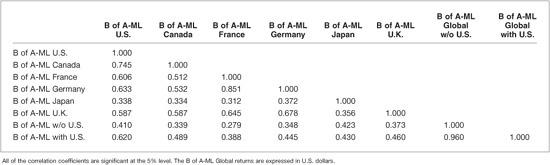
Exhibit 3–8 contains correlations among returns in U.S. dollars. The results differ from local currency results and normal expectations. Typically, correlations decline when one goes from local currency to U.S. currency because of the effect of random exchange-rate changes, which reduce the relationships. As expected, this decline in correlations occurred among all these countries and the United States, and it also happened for all correlations with Canada. In contrast, the correlations among the European countries and for these countries with Japan consistently experienced large increases when returns were in U.S. dollars, and all the correlations with the global indexes increased substantially. For example, the correlations between France and Germany went from about 0.85 to 0.97. This implies that during this period, the exchange-rate correlations were quite high and became a cause for stronger return correlations. In addition, the European Union currency was initiated on January 1, 1999, which had an impact on the recent results.
EXHIBIT 3–8
Correlation Coefficients among Monthly Global Government Bond Index Returns in U.S. Dollars (1986–2010)
KEY POINTS
• Bond market indexes are important for those who analyze bonds or manage bond portfolios because they have several significant uses, including acting as performance benchmarks, a benchmark for investors who want to invest through index funds, and a means to determine fixed income asset risk/return characteristics and correlations as inputs into the asset allocation decision.
• A brief analysis of the risk/return characteristics of alternative bond series indicates that most of the series had results in line with expectations. The outliers are the very risky securities (Caa bonds and defaulted bonds), which underperformed, while low-risk high-yield bonds (Ba rated), outperformed. The global bond results are heavily affected by the currency effect. Local currency results are consistent, except for Japan, which was below the market line. The U.S. dollar results were quite consistent in terms of risk and return, with most countries showing benefits from the weak dollar. The global index results were in line with most country results.
• The analysis of correlations for U.S. bond indexes indicates that there are very high correlations among bond series within either the investment-grade or the high-yield bond sector (typically between 0.79 and 0.99). In contrast, there are significantly lower correlations between investment-grade and high-yield bonds (with correlations typically between 0.20 and 0.40.) Defaulted debt had no correlation with investment-grade debt but fairly significant correlation with high-yield debt.
• The correlations among the global indexes in local currencies typically show fairly low relationships with other countries (about 0.50), except United States–Canada and France–Germany (between 0.75 and 0.85). The correlations changed when we considered returns in U.S. dollars. Specifically, all the correlations with the United States declined, whereas many of the correlations among non-U.S. countries increased owing to the weak U.S. dollar during this period, which affected these countries simultaneously—and the introduction of European Union currency.
• The significance of many of the empirical results of risk/return and correlations is limited because of the relatively short 25-year time period. Although these results do not have the long history one would want, the important point is that it is currently possible to do serious analysis of the bond market because there are a number of very well-constructed and diverse bond indexes available, as described herein. Such an analysis of the bond market and its components is critical for investors and portfolio managers making asset allocation and portfolio-performance decisions.