
CHAPTER
TWENTY-NINE
SUPPORT BONDS WITH SCHEDULES IN AGENCY CMO DEALS
Principal
OffStreet Research LLC
Collateralized mortgage obligations (CMOs) were first devised to meet two general objectives. The first was to make a better match between a wide range of investors’ maturity requirements and the expected cash flows from a pool of mortgages. The second was to redistribute prepayment risk to different classes at levels that many more investors would accept. The initial solution to the problem simply split the returning principal among a series of sequential-pay bonds. Subsequently, this structure has evolved into an array of reduced-risk CMO bond structures, the most heavily issued of which is the planned amortization class (PAC). PACs provide investors with payments scheduled as to payment date and amount, occurring within a defined paydown period (window), and protected over a range of likely prepayment scenarios.
Support bonds, also known as support bonds, are the natural by-product of creating PAC bonds.1 In order to protect the schedules of PAC bonds in a CMO issue, a sufficient amount of bond classes must be created to absorb excess principal paydowns and to provide a buffer from which scheduled payments can be made when prepayments are slow. Because support bond classes accept additional prepayment volatility, their payments are necessarily more uncertain than either PACs or traditional CMO bonds. As a result, the actual yields or economic returns realized from an investment in support bonds can vary widely from those projected at the time of investment. Investors recognize this risk, and they demand yields that compensate them accordingly.
Issuers and underwriters also have developed a variety of devices that serve either to reduce the risk of a portion of the support bond classes or to create more volatile instruments that reward holders when interest rates (and presumably prepayment rates) move strongly in a particular direction. Lockouts2 are among the first group, while super-POs and jump Zs are typical of the second. Another very common strategy is to create support bonds with floating and inverse floating-rate coupons. One of the oldest and most extensively employed strategies, however, is to give schedules to a portion of the support bond cash flows and to provide those schedules with more limited prepayment protection than the primary PAC series receive. This family of reduced-risk support bonds is the subject of this chapter.
Support bonds having schedules partake either of the properties of targeted amortization classes (TACs)—so that they are protected against either call or extension risk (a reverse TAC) but not both—or of PAC bonds, so that they have call and extension protection over a range of prepayment scenarios (a Level II PAC). The concept of Level II PACs took hold during the third quarter of 1989. In the early 1990s, it became common to create several levels of PACs with successively narrower bands of prepayment protection, so that a single transaction could contain PAC Is, IIs, and IIIs. In addition, the practice of carving a “super-PAC” schedule out of a primary PAC schedule became popular.
The following discussion explains how support PAC and TAC bonds are structured and how their structures affect their performance in different prepayment scenarios. The effect of adding a TAC, reverse TAC, or Level II PAC on the behavior of the remaining support bonds is also explored.
SUPPORT BOND BASICS
Support bond classes are created from the principal payments remaining after the PAC schedules are defined. In general, support bond classes have second claim on excess principal paid down from the collateral after the PAC schedules, and pay sequentially until all the support bonds are retired. At the pricing prepayment assumption, support bond classes pay simultaneously with the PACs. At very slow constant prepayment rates, they must wait to receive principal until the PACs have been retired. At very high constant speeds, they pay simultaneously with the short-term average life PACs and are quickly retired, after which the PACs themselves must absorb excess paydowns and are retired ahead of schedule.
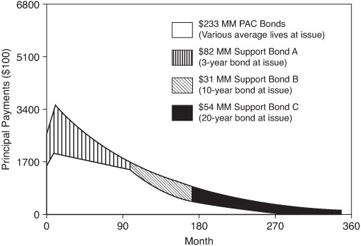
A simplified example of a standard PAC-support bond structure is depicted in Exhibit 29–1. The large unshaded area paying from the first to about the 300th month contains all the scheduled payments that would be available to construct PAC bonds, assuming collars of 85% and 300% PSA.3 Normally, structurers would divide this PAC region into a number of PACs with varying average lives. The actual number of PACs created would depend on the demand for particular maturities and windows (the time elapsed between first and last principal payments to the PAC bondholders). For ease of exposition, the PAC region in this and subsequent examples is not divided. The support bonds are not influenced by the partitioning of a single PAC region into individual bond classes; they are affected, instead, by the size of the entire PAC region in relation to the total size of the support bond classes. (In general, the larger the PAC class, given a fixed amount of collateral, the more volatile the support bond class is.) The principal payments left over after the PAC region is defined constitute the support bond classes. In Exhibit 29–1, these are depicted by the shaded areas. At a pricing prepayment assumption of 165% PSA, the support bonds pay sequentially over the entire remaining life of the collateral. In this example the support bond paydowns at 165% PSA have been divided into three classes with average lives of 3.1, 11.5, and 20.3 years (nominally a series of 3-, 10- and 20-year bonds).
EXHIBIT 29–1
PAC with Standard Support Bonds, 165% PSA
The impact of actual prepayment experience on the size and timing of principal payments to the support bond classes is graphically depicted in Exhibits 29–2 and 29–3. When prepayments occur at a constant speed of 300% PSA (the upper PAC collar), as shown in Exhibit 29–2, the PAC schedule is not disturbed, but the support bonds shorten dramatically and are all fully retired by the 8th year. By contrast, when prepayments slow to 85% PSA (the lower PAC collar), the first support bond does not begin to pay until about the 8th year, as Exhibit 29–3 indicates. The resultant average life volatility is very significant. Bonds with average lives at pricing of 3, 10, and 20 years shorten to 1.0, 2.5, and 5.8 years, respectively, at 300% PSA; and at 85% PSA, the bonds have average lives of 15.0, 21.1, and 25.6 years, respectively.
EXHIBIT 29–2
PAC with Standard Support Bonds, 300% PSA

EXHIBIT 29–3
PAC with Standard Support Bonds, 85% PSA

The average life variability of a support bond is generally a function of the size of the PAC region relative to the entire issue, the size of the support bond relative to the remaining support bonds, and its average life at the pricing prepayment assumption. A detailed examination of how these characteristics interact to produce the actual behavior of support bonds in different prepayment scenarios is beyond the scope of this chapter. Still, it is worth outlining the basic relationships between support bond structure and behavior because they apply as well to the more complex, schedule-based structures that are the subject of this chapter.
The order in which a support bond is scheduled to receive excess cash flows also can profoundly affect its average life behavior. It is normally assumed that support bonds will be retired in the order of their average lives at issue and that this order of priority does not change over the term of the transaction (indeed, that assumption is made throughout this discussion). This assumption, however, could be altered, generating results that are entirely specific to the transaction in question. Rather than assume that a certain order of priorities is standard, investors should assure themselves that they understand the priorities and other rules on which the structure is based, as well as the conditions under which they may be switched on or off.
There are basically three different ways to vary the relative size of the support bonds. Lockouts, already mentioned above, are typically employed to improve the stability of payments to the earliest support bond class in the issue. Moreover, with two or three years of schedulable paydowns added to its size, the first support bond can provide a larger buffer against call and extension for subsequent support bonds. A similar technique is to pay the later years or “tail” of the PAC schedule to the support bonds projected to be paying at the same time. Intermediate- or long-term support bonds can benefit from this technique. The third, tightening the collars, can increase the size of the support bonds.
Raising the bottom collar increases the principal available for support bond classes in the early years (generally the first quarter to first third of the remaining term of the collateral), and lowering the top collar increases principal in later years.
It also should be apparent that the smaller the scheduled PAC payments, the more principal will be available to make payments to support bonds at any given prepayment speed. This means that extension risk is reduced; call risk is also reduced. The smaller the PAC region, the larger the projected paydowns to the support bond in any one period and the smaller the excess principal as a proportion of the projected support bond principal payment will be. In other words, excess principal has a proportionally smaller impact on the dollar weights used to compute the support bond’s average life.
For similar algebraic reasons, changing the proportion of PACs, while holding the average lives about the same, has a bigger impact on the volatility of support bonds constructed from cash flows at the tail, because smaller dollar weights are applied to later dates. The absolute magnitude of the average life at issue of a support bond also determines how much it can lengthen or shorten. This is also very intuitive: The longer the average life at issue, the less room to lengthen and the more room to shorten. Similarly, short-term bonds have less room to shorten, more to lengthen.
The shortening of a CMO bond’s average life in a bull market or, conversely, its lengthening in a bear market generally are negative events from the investor’s point of view. Two effects are of particular concern. For one, the additional cash-flow accelerates or decelerates at the wrong time. As a consequence of the interest rate sensitivity of the prepayment process, reinvestment opportunities are most likely to have declining yields when prepayments are increasing, and rising yields when prepayments are drying up. Second, as average life varies, so too does the bond’s duration or price sensitivity. In a bull market, the bond’s price appreciates more slowly as market yields decline, generating a lower economic return than a bond of like but stable average life. In a bull market, the support bond’s value depreciates more quickly as yields rise.4
Since support bonds absorb additional volatility from the protected bonds, changes in expected average life resulting from changes in prepayment experience in the collateral are of heightened concern to investors who hold them. As crucial as an accurate model of the prepayment process is for anticipating the performance of other mortgage-related products in various interest rate scenarios, it is even more valuable in the evaluation of support bonds. Without appropriate prepayment projections, such as can be derived from an econometric prepayment model, it is not possible to link changes in interest rate levels to meaningful estimates of the yield or total rate of return of a support.
SUPPORT TAC BONDS
Since their introduction in the third quarter of 1988, support TAC bonds have proved to be a highly marketable innovation. Indeed, since the first TACs were issued, the market has evolved away from TAC-only structures to prefer support TAC bonds. Clean TAC bonds (from structures without PACs) tend to be offered less frequently.
A TAC schedule is created by projecting the principal cash flows for the collateral at a single constant prepayment speed. This speed is typically the prepayment speed at which the bonds are priced. In the case of a clean TAC, the projected principal payments define the schedule. In the case of the support bond, TAC, the TACs are constructed from projected principal remaining after scheduled PAC payments are made. The TACs have first priority after the PACs to principal payments, and their schedules are protected from call risk by the existence of other support bond classes that absorb any principal paydowns that exceed both the scheduled PAC and TAC payments in any period. The larger these “support” classes are in relation to the support TAC bond, the greater the protection provided to the TAC schedule.
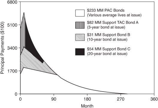
Compared to a clean TAC with similar (in the example they are the same) average life and underlying collateral, the support TAC bond necessarily receives less protection, because a larger proportion of the total collateral has already been allocated to high-priority PAC bonds, and a much smaller proportion of principal remains to be allocated to lower-priority support tranches. For this discussion, a simplified example of a support TAC bond was created from the 3-year support bond in Exhibit 29–1. This was done simply by defining a schedule as the principal payments to the 3-year support bond, assuming a constant prepayment speed of 165% PSA. Since it is identical at 165% PSA to the PAC-standard support bond example, readers should refer to the cash-flow diagram in Exhibit 29–1 to understand this structure. The impact of faster prepayments on this PAC-TAC structure is shown in Exhibit 29–4. At 300% PSA, the higher priority given the TAC schedule forces the 10- and 20-year support bonds to pay down simultaneously with the TAC (instead of sequentially as in Exhibit 29–2). Readers will note that the shape of the support TAC bond at 300% PSA is almost but not entirely identical to its shape at 165%, indicating that the schedule is still well protected at this speed. The size and timing of later payments has been altered slightly at the higher prepayment speed for reasons discussed below.
EXHIBIT 29–4
PAC with Standard Support TAC, 300% PSA
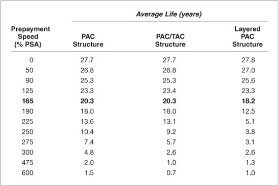
Support TAC bonds generally have the same properties as clean TACs: They provide a degree of call protection and little extension protection. Many structures actually will first extend, when prepayments slightly exceed the TAC speed, before shortening at higher speeds. The important difference is that support TAC bonds have significantly less call protection since they must absorb excess principal once the remaining unscheduled support bonds are retired. This can be seen by examining Exhibit 29–5, in which the average lives of various 3-year CMO bonds at various prepayment speeds are compared. For comparison, a clean TAC with a 3.1-year average life has been constructed from the same collateral used to create the PAC-standard support bond and PAC-TAC examples. The clean TAC has unnaturally exceptional call protection (it is protected by $360 million of support bonds, which comprise the remainder of the structure). The smaller size of the clean TAC also results in its having a lower average life at very low prepayment speeds than the support TAC bond does (the clean TAC is small enough for even small paydowns at low speeds to reduce its principal balance significantly in the early years).
EXHIBIT 29–5
Average Lives at Various Prepayment Speeds of Different 3-Year PAC-Support Bond Structures (Pricing Assumption 165% PSA)

The more important comparison, since so few clean TACs are issued at present, is with the 3-year support bond from Exhibits 29–1, 29–2, and 29–3. The support TAC bond clearly provides meaningful call protection, requiring speeds in excess of 600% PSA before it shortens as much as the standard support bond does at 300% PSA. The two bonds extend identically. This happens because they both have the same priority after the PACs to receive principal paydowns and no support bonds in front of them (the TAC would have priority over an earlier support bond, which would protect it to a degree from extending, whereas the standard support bond would wait until earlier support bonds were retired, which would cause it to extend).
Notice that at 300% PSA, the support TAC bond’s average life is about a month longer than at the pricing speed (rounding exaggerates the difference—at several more places of significance the difference is really about 0.08 year). This phenomenon occurs at relatively high speeds, since principal payments become more bunched in the early months and trail off more sharply in later months. Exhibit 29–4, as mentioned above, gives some indication of what is happening at this speed to the principal cash flows thrown off by the collateral. The paydowns become more “tailish” toward the end of the support bond’s schedule, forcing it to wait as excess payments are, going into the tail, not large enough to meet the schedule.
The other great difference between PAC-TAC structures and both clean TAC and PAC-standard support bond structures is how much more volatile the unscheduled support bonds can be. The presence of additional risk-reduced structures forces the remaining support bonds to absorb more prepayment volatility. This is demonstrated in Exhibit 29–6, where various 20-year support bond structures are compared. At prepayment speeds above 225% PSA, the support bond in the PAC-TAC structure begins to shorten much more quickly than the standard support bond.
EXHIBIT 29–6
average Lives at Various prepayment Speeds of 20-Year Support Bond from Different CMO Structures (pricing assumption 165% PSA)
REVERSE TACs
Payment rules and priorities also can be devised that protect a support bond from extension risk while leaving it more exposed to call risk. These structures fittingly are termed “reverse TACs.” Reverse TACs are more likely to be created when bearish sentiment is strong. These structures typically are created as 20-year support bond classes. Their long lives make them natural candidates for this treatment, as they have not, in any case, more than six or maybe eight years to extend. Additionally, these structures are priced at significant discounts from par in order to benefit from increases in prepayments.
An example of a reverse TAC was created for this discussion by defining a payment schedule for the fourth tranche of the PAC-support bond structure depicted in Exhibits 29–1, 29–2, and 29–3. A cash-flow diagram for prepayments at 85% PSA is included in Exhibit 29–7. (At 165% PSA and faster speeds, the PAC-reverse TAC structure, as will be explained, pays exactly like the PAC-standard support bond, which is depicted at 165% PSA in Exhibit 29–1 and 300% PSA in Exhibit 29–3.) The schedule was run at 165% PSA, the pricing speed in all these examples, and has priority after the scheduled PAC payments are made. The reverse TAC receives excess cash-flow only after the 3- and 10-year support bonds are retired. These arrangements preserve the schedule at prepayment speeds slower than those used to generate the schedule, but not at faster speeds. The reverse TAC does not begin to extend until prepayments fall below a constant rate of about 70% PSA.
The average life volatility of the reverse TAC is compared to that of other 20-year support bond structures in Exhibit 29–8. The reverse TAC in the example has an average life of 20.3 years; in the worst case, that of no prepayments, the bond’s average life only extends to 24.5 years. By comparison, the last tranche of the simple structure extends to 27.7 years. The cash-flow diagrams in Exhibits 29–3 and 29–7 make it clear why this is so. In the simple PAC-support bond structure (Exhibit 29–3), at a speed equal to the upper collar, the support bonds pay down sequentially after the PAC bonds are retired. In the structure with the reverse TAC (Exhibit 29–7), the 3-and 10-year support bonds extend to permit the scheduled reverse TAC payments to be met. At 85% PSA, the lower PAC collar, the short-and intermediate-term support bonds pay simultaneously with the reverse TAC. At slower prepayment speeds, the average lives of both support bonds exceed that of the reverse TAC.
EXHIBIT 29–7
PAC with Reverse TAC Bond, 85% PSA
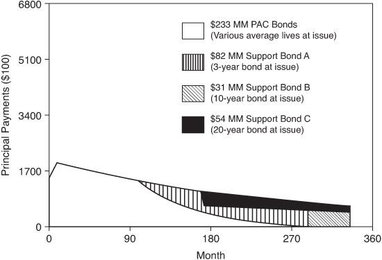
EXHIBIT 29–8
Average Lives at Various Prepayment Speeds of 20-Year Support Bonds from Different PAC-Support Structures (Pricing Assumption 165% PSA)
The reverse TAC imparts considerably more volatility to the other support bonds when prepayments slow, but it does not cause them to be more volatile in faster prepayment scenarios. This effect can also be seen by comparing the average lives of 3-year support bonds from both structures listed in Exhibit 29–9. This is a natural consequence of the one-sided protection afforded by targeted amortization structures.
Schedules can also be applied to intermediate-term support bonds to protect their average lives from extending in slow prepayment scenarios. At the same time, the structure is “protected” from call risk in moderately fast prepayment scenarios by taking advantage of the natural tendency of TACs to extend slightly as prepayments exceed the pricing speed. The resulting average life profile can be reasonably stable across a significant range of prepayment speeds (for example, extending no more than 2 or 3 years across a range from 50% or 75% PSA to 225% or 250% PSA, assuming a schedule run at 165% PSA). In effect, an intermediate-term support TAC bond can be constructed to provide PAC-like stability. A number of such bonds have indeed been issued, some of them with monikers indicating that the payments are stabilized or controlled.
EXHIBIT 29–9
Average Lives at Various Prepayment Speeds of 3-Year Structured Supports from Different PAC-Support Structures (Pricing Assumption 165% PSA)

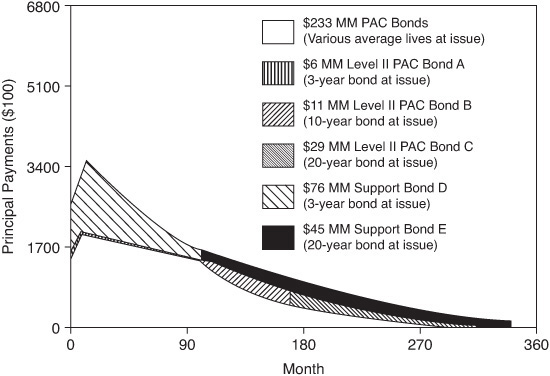
LAYERED PAC BONDS
The value of support bond classes also can be enhanced by establishing secondary PAC schedules for a portion of the principal remaining after the primary PAC payments are met. A cash-flow diagram for an example of a two-tiered PAC structure, run at a pricing speed of 165% PSA, is shown in Exhibit 29–10. This example uses the same collateral as the previous examples. The same collars—85% to 300% PSA—were used to create the same amount of primary or Level I PACs—$233.0 million of a total original balance of $400 million CMO bonds. Collars for the second tier of PACs were set at 90% to 225% PSA. The second-tier PAC region was further divided into a series of nominally 10- and 20-year bonds and the support bonds into 3- and 20-year bonds. (In order to match the 3.1-year average lives in the previous examples, it was necessary to let the long-term bonds in the layered PAC example have average lives closer to 18 than to 20 years. This does not vitiate the comparison.) The Level II PACs (also called PAC 2s) appear in the figure as a narrow band between the PAC region and the support bonds: At 165% PSA they pay down simultaneously with the primary PACs in the deal. The size of the second tier of PACs is a function of the collars—the tighter the protection band, the larger the amount of PACs that can be created. In this example, protecting the Level II schedule up to 225% PSA limits the amount of 3-year Level II PACs that can be created to $5.6 million. In total, the second layer of PACs only amount to about 11% of the transaction (58.25% of the transaction is standard, Level I PACs).
EXHIBIT 29–10
Layered PAC Structure, 165% PSA
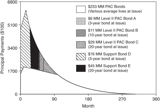
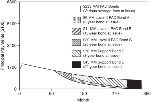
The Level II PAC schedule remains intact until prepayment speeds break the primary PAC collars. For example, Exhibit 29–11 shows the principal payments at 300% PSA. At this speed, the primary PAC schedule is not violated, but payments to the Level II PACs are significantly accelerated, shortening to average lives of 2.5, 3.9, and 5.8 years, respectively. Similarly, when prepayments slow to a constant speed of 85% PSA, primary PAC payments are made on schedule, but the payments to Level II PACs are delayed. At 85% PSA, as shown in Exhibit 29–12, the support bond PACs have average lives of 9.5, 11.3, and 18.1 years, respectively. As would be expected, the longer Level II PACs are more volatile on the upside, when prepayments accelerate, and the shorter PACs are more volatile on the downside, when prepayments decelerate. The 3- and 20-year support bonds receive no principal until the Level II PACs are paid, extending their average lives to 18.3 years and 25.6 years, respectively.
EXHIBIT 29–11
Layered PAC Structure, 300% PSA
The average life volatility of Level II PACs is compared to that of support TAC bonds and 3-year standard support bonds in Exhibit 29–6. Although not as well protected as primary PACs, Level II PACs do provide modest call protection and decent extension protection. Moreover, these examples demonstrate that they can shorten and extend less vigorously than their TAC and reverse-TAC counterparts when prepayments move outside the appropriate protective boundary. The support bonds of layered PACs are somewhat more volatile over moderate prepayment shifts. As the comparison in Exhibit 29–8 with a 20-year standard support TAC bond and a reverse TAC suggests, the 20-year layered support TAC bond shortens faster between 165% and about 250% PSA than either of its counterparts. Similarly, Exhibit 29–9 indicates that the 3-year layered support TAC bond lengthens more abruptly than its counterparts at prepayment speeds between 165% and 50% PSA.5
EXHIBIT 29–12
Layered PAC Structure, 85% PSA
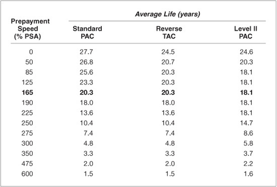
SUMMARY OF AVERAGE LIFE VOLATILITIES
The average life volatilities of the 3-year support bond structures discussed in this chapter are summarized in Exhibit 29–13, as are those of the 20-year support bonds in Exhibit 29–14. The graphs make plain the differences in call and extension protection that can be provided by furnishing support bond classes with TAC or PAC schedules. The Level II PACs have stable average life patterns between the upper and lower collar speeds. (A Level I PAC would have a similar pattern, only it would be stable over a wider range, say 75% to 300% PSA, and owing to the presence of the support bonds, would shorten or lengthen more moderately outside that range.) By comparison, the standard support bonds demonstrate steep and continuous changes in average life over the same ranges for which the Level II PACs are protected. The TACs, as would be expected, provide call protection, but no extension protection, while the reverse TACs are stable at slower speeds, but shorten abruptly when prepayments occur at faster constant rates than the prepayment assumption.
EXHIBIT 29–13
Different 3-Year CMO Support Bond Structures (Average Lives over a Range of Constant Prepayment Speeds)
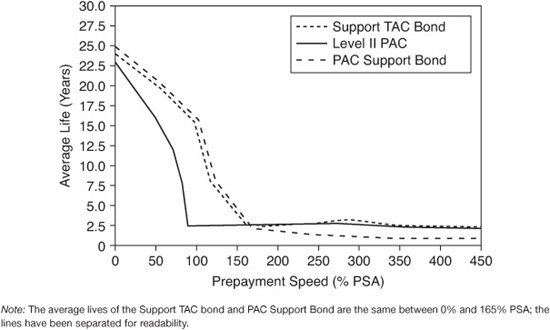
EXHIBIT 29–14
Different 20-Year CMO Support Bond Structures (Average Lives over a Range of Constant Prepayment Speeds)

KEY POINTS
• Support PAC bonds having schedules partake either of the properties of TACs—so that they are protected against either call or extension risk (a reverse TAC) but not both—or of PAC bonds, so that they have call and extension protection over a range of prepayment scenarios (a Level II PAC).
• Although not as well protected as primary PACs, support PAC bonds with a schedule (also known as Level II PACs) provide modest call protection and decent extension protection.
• Level II PAC schedule remains intact until prepayment speeds break the primary PAC collars.
• Level II PACs shorten and extend less vigorously than their TAC and reverse-TAC counterparts when prepayments move outside the appropriate protective boundary. The support bonds of layered PACs are somewhat more volatile over moderate prepayment shifts.