CHAPTER
THIRTY-SEVEN
A FRAMEWORK FOR ANALYZING YIELD-CURVE TRADES

ANTTI ILMANEN, PH.D.

Managing Director
AQR Capital Management (Europe) LLP

In Chapter 36, it was explained that the shape of the yield-curve depends on three main determinants: the market’s rate expectations, the required bond risk premia, and the convexity bias. In this chapter we show how to decompose the forward rate curve into these three determinants. Even though we cannot observe these determinants directly, the decomposition can clarify our thinking about the yield-curve.

Our analysis also produces direct applications—it provides a systematic framework for relative-value analysis of noncallable government bonds. Analogous to the decomposition of forward rates, the total expected return of any government bond position can be viewed as the sum of a few simple building blocks: (1) the yield income, (2) the rolldown return, (3) the value of convexity, and (4) the duration impact of the rate view. A further term should be added for bonds that trade “special” in the repo market and for bonds that trade very rich or cheap against the fitted curve.

The following observations motivate this decomposition. A bond’s near-term expected return is a sum of its horizon return given an unchanged yield-curve and its expected return from expected changes in the yield-curve. The first item, the horizon return, is also called the rolling yield because it is a sum of the bond’s yield income and the rolldown return (the capital gain that the bond earns because its yield declines as its maturity shortens and it “rolls down” an upward-sloping yield-curve). The second item, the expected return from expected changes in the yield-curve, can be approximated by duration and convexity effects. The duration impact is zero if the yield-curve is expected to remain unchanged, but it may be the main source of expected return if the rate predictions are based on an investor’s or economist’s market view or on a quantitative forecasting model. The value of convexity is always positive and depends on the bond’s convexity and on the perceived level of yield volatility.

This chapter is a revised version of a Citigroup (Salomon Brothers) research report. Such report remains the property of Citigroup, and its disclaimers apply.

We argue that both prospective and historical relative-value analysis should focus on near-term expected-return differentials across bond positions instead of on yield spreads. The former measures are more comprehensive in the sense that they take into account all sources of expected return. Moreover, they provide a consistent framework for evaluating all types of government bond positions. We also show, with practical examples, how various expected-return measures are computed and how our framework for relative-value analysis is related to the better-known scenario analysis.

FORWARD RATES AND THEIR DETERMINANTS

Chapter 36 shows that the yield-curve can be represented in either par rates, spot rates, or forward rates. Whichever representation is used, there are three main determinants of the yield-curve that we discuss next.

How Do the Main Determinants Influence the Yield-Curve Shape?

We describe here how the market’s rate expectations, the required bond risk premia,¹ and the convexity bias influence the term structure of interest rates. The market’s expectations regarding the future interest-rate behavior probably are the most important influences on today’s term structure. Expectations for parallel increases in yields tend to make today’s term structure linearly upward sloping, and expectations for falling yields tend to make today’s term structure inverted. Expectations for future curve flattening induce today’s spot- and forward-rate curves to be concave (functions of maturity), and expectations for future curve steepening induce today’s spot- and forward-rate curves to be convex.² These are the facts, but what is the intuition behind these relationships?

The traditional intuition is based on the pure expectations hypothesis. In the absence of risk premia and convexity bias, a long rate is a weighted average of the expected short rates over the life of the long bond. If the short rates are expected to rise, the expected average future short rate (i.e., the long rate) is higher than the current short rate, making today’s term structure upward-sloping. A similar logic explains why expectations of falling rates make today’s term structure inverted. However, this logic gives few insights about the relation between the market’s expectations regarding future curve reshaping and the curvature of today’s term structure.

Another perspective to the pure expectations hypothesis may provide a better intuition. The absence of risk premia means that all bonds, independent of maturity, have the same near-term expected return. Recall that a bond’s holding-period return equals the sum of the initial yield and the capital gains/losses that yield changes cause. Therefore, if all bonds are to have the same expected return, initial yield differentials across bonds must offset any expected capital gains/losses. Similarly, each bond portfolio with expected capital gains must have a yield disadvantage relative to the riskless asset. If investors expect the long bonds to gain value because of a decline in interest rates, they accept a lower initial yield for long bonds than for short bonds, making today’s spot- and forward-rate curves inverted. Conversely, if investors expect the long bonds to lose value because of an increase in interest rates, they demand a higher initial yield for long bonds than for short bonds, making today’s spot- and forward-rate curves upward-sloping. Similarly, if investors expect the curve-flattening positions to earn capital gains because of future curve flattening, they accept a lower initial yield for these positions. In such a case, barbells would have lower yields than duration-matched bullets (to equate their near-term expected returns), making today’s spot- and forward-rate curves concave. A converse logic links the market’s curve-steepening expectations to convex spot- and forward-rate curves.

The preceding analysis presumes that all bond positions have the same near-term expected returns. In reality, investors require higher returns for holding long bonds than short bonds. Many models that acknowledge bond risk premia assume that they increase linearly with duration (or with return volatility) and that they are constant over time. Empirical evidence contradicts both assumptions.³ Historical average returns increase substantially with duration at the front end of the curve but only modestly beyond intermediate durations. Thus the bond risk premia make the term structure upward-sloping and concave, on average. Moreover, it is possible to forecast when the required bond risk premia are abnormally high or low. Thus the time variation in the bond risk premia can cause significant variation in the shape of the term structure.

Convexity bias refers to the impact that the nonlinearity of a bond’s price/yield-curve has on the shape of the term structure. This impact is very small at the front end but can be quite significant at very long durations. A positively convex price/yield-curve has the property that a given yield decline raises the bond price more than a yield increase of equal magnitude reduces it. All else equal, this property makes a high-convexity bond more valuable than a low-convexity bond, especially if the volatility is high. It follows that investors tend to accept a lower initial yield for a more convex bond because they have the prospect of enhancing their returns as a result of convexity. Because a long bond exhibits much greater convexity than a short bond, it can have a lower yield and yet offer the same near-term expected return. Thus, in the absence of bond risk premia, the convexity bias would make the term structure inverted. In the presence of positive bond risk premia, the convexity bias tends to make the term structure humped—because the negative effect of convexity bias overtakes the positive effect of bond risk premia only at long durations. An increase in the interest-rate volatility makes the bias stronger and thus tends to make the term structure more humped.

The three determinants influence the shape of the term structure simultaneously, making it difficult to distinguish their individual effects. Despite a widespread misconception, the shape of the term structure does not reflect only the market’s rate expectations. Forward rates are good measures of the market’s rate expectations only if the bond risk premia and the convexity bias can be ignored. This is hardly the case, even though a large portion of the short-term variation in the shape of the curve probably reflects the market’s changing expectations about the future level and shape of the curve. The steepness of the curve on a given day depends mainly on the market’s view regarding the rate direction, but in the long run, the impact of positive and negative rate expectations largely washes out. Therefore, the average upward slope of the yield-curve is mainly attributable to positive bond risk premia. The curvature of the term structure may reflect all three components. On a given day, the spot-rate curve is especially concave (humped) if market participants have strong expectations of future curve flattening or of high future volatility. In the long run, the reshaping expectations should wash out, and the average concave shape of the term structure reflects the concavity of the risk premium curve and the convexity bias.

Decomposing Forward Rates into Their Main Determinants

Conceptually, each one-period forward rate can be decomposed to three parts: the impact of rate expectations, the bond risk premium, and the convexity bias. So far this statement is just an assertion. In this subsection we show intuitively why this relationship holds between the forward rates and their three determinants. We provide a more formal derivation in Appendix 37A (where we take into account the fact that the analysis is not instantaneous but that yield changes occur over a discrete horizon, during which invested capital grows). In Appendix 37B we tie some loose strings together by summarizing various statements about the forward rates and by clarifying the relations between these statements.

Exhibit 37–1 shows how the yield change of an n-year zero-coupon bond over one period (dashed arrow) can be split to the rolldown yield change and the one-period change in an n − 1 year constant-maturity spot rate (two solid arrows).⁴ A zero-coupon bond’s price can be split in a similar way (see Appendix 37A). Thus an n-year zero’s holding-period return over the next period h_n is

EXHIBIT 37–1
Splitting a Zero-Coupon Bond’s One-Period Yield Change into Two Parts

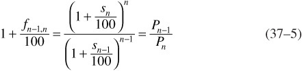
Equation (37–1) is based on the following relations. First, a bond’s one-period horizon return given an unchanged yield-curve is called the rolling yield. A zero-coupon bond’s rolling yield equals the one-period forward rate (f_n−_1,n). For example, if the four-year (five-year) constant-maturity rate remains unchanged at 9.5% (10%) over the next year, a five-year zero bought today at 10% can be sold next year at 9.5% as a four-year zero; then the bond’s horizon return is 1.10⁵/1.095⁴ - 1 = 0.1202 = 12.02%, which is the one-year forward rate between four- and five-year maturities [see Eq. (37–11) in Appendix 37B]. The second source of a zero’s holding-period return, the price change caused by the yield-curve shift, is approximated very well by duration and convexity effects for all but extremely large yield-curve shifts.

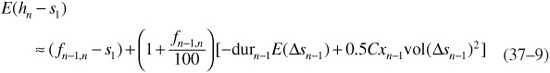
It is more interesting to relate the forward rates to expected returns and expected rate changes than to the realized ones. We take expectations of both sides of Eq. (37–1), split the bond’s expected holding-period return into the short rate and the bond risk premium, and recall that E(Δs_n–₁)² ≈ [vol(Δs_n–₁)]². Then we can rearrange the equation to express the one-period forward rate as a sum of the other terms:

where bond risk premium = E(h_n − s₁), and convexity bias ≈ −0.5 × convexity × [vol(Δ_n−1)]².

If we move the short rate to the left-hand side of the equation, we decompose the “forward-spot premium” (f_n−1,n − s₁) into a rate-expectation term, a risk-premium term, and a convexity term (see Eq. 37–10 in Appendix 37A). We interpret the expectations in Eq. (37–2) as the market’s rate and volatility expectations and as the expected risk premium that the market requires for holding long-term bonds. The market’s expectations are weighted averages of individual market participants’ expectations.

Some readers may wonder why our analysis deals with forward rates and not with the more familiar par and spot rates. The reason is the simplicity of the one-period forward rates. A one-period forward rate is the most basic unit in term-structure analysis, the discount rate of one cash-flow over one period. A spot rate is the average discount rate of one cash-flow over many periods, whereas a par rate is the average discount rate of many cash-flows—those of a par bond—over many periods. All the averaging makes the decomposition messier for the spot rates and the par rates than it is for the one-period forward rate in Eq. (37–2). However, because the spot and the par rates are complex averages of the one-period forward rates, they too can be decomposed conceptually into the three main determinants.

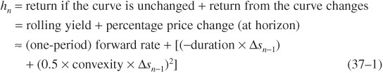
Because the approximate decomposition in Eq. (37–2) is derived mathematically without making specific economic assumptions, it is true in general. In reality, however, it is hard to make this decomposition because the components are not observable and because they vary over time. Further assumptions or proxies are needed for such a decomposition. In Exhibit 37–2 we use historical average returns to compute the bond risk premia and historical rate volatilities to compute the convexity bias—together with the observable market forward rates (as of April 2004)—and back out the only unknown term in Eq. (37–2): the expected spot-rate change times duration. We also could divide this term by duration to infer the market’s rate expectations. The rate expectations that we back out in Exhibit 37–2 suggest that the market expects rising short rates but less than forwards imply.

EXHIBIT 37–2
Decomposing Forward Rates into Their Components Using Historical Average Risk Premia and Volatilities

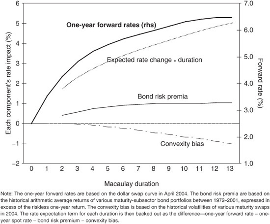
If bond risk premia vary over time, the use of historical average risk premia may be misleading. As an alternative, we can use survey data or rate predictions based on a quantitative forecasting model to proxy for the market’s rate expectations. In Exhibit 37–3, we use a hypothetical consensus interest-rate forecast that predicts a bear flattening (yields rising 100 basis points at the two-year maturity and 20 basis points at ten years). In addition, we use implied volatilities from swaption prices to compute the convexity bias. These components can be used together with the one-year forward rates to back out estimates of the unobservable bond risk premia.

EXHIBIT 37–3
Decomposing Forward Rates into Their Components Using Hypothetical Survey Rate Expectations and Implied Volatilities

A comparison of Exhibits 37–2 and 37–3 shows that the two decompositions look similar at short durations but different at intermediate and long durations. The similarity of the convexity bias components in these two exhibits suggests that the use of historical or implied volatilities makes little difference, at least in this case. The hypothetical survey’s yield-curve view implies a relatively poor performance of intermediate-duration assets (low expected excess return) and a good performance by the longest assets (whose yields are expected to be stable). Because the forward-rate curve is the same in both exhibits, any smaller predicted rate increases lead to higher bond risk premia in Exhibit 37–3 than in Exhibit 37–2.⁵

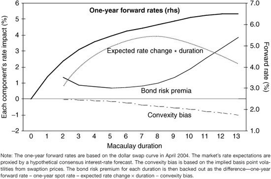
Exhibits 37–2 and 37–3 are snapshots of the forward rates and their components on one date. A comparison of similar decompositions over time would provide insights into the relative variability of each component. In Exhibit 37–4, we try to illustrate the impact of changing rate expectations and risk premia on the steepness of the U.S. Treasury bill curve based on a semiannual survey of economists’ rate forecasts. The exhibit shows that the forwards almost always implied larger increases in the three-month rate than the market expected, based on surveys of bond market analysts. The difference is proportional to the required bond risk premium of longer bills over shorter bills (because bills exhibit negligible convexity, its impact can be ignored). This difference clearly varies over time.

The time variation in the survey-based bond risk premium in Exhibit 37–4 appears economically reasonable. It fell secularly from the early 1980s to late 1990s, perhaps reflecting the trend decline in inflation expectations and in level-dependent inflation uncertainty. Besides the lower inflation risk premium, improving fiscal prospects likely contributed to this trend decline. The bond risk premium also exhibited cyclic fluctuations that are related to the direction of consensus rate predictions and thus the central bank’s policy tightening and easing cycles. Finally, the bond risk premium turned slightly negative during the flight to quality in late 1998, arguably reflecting government bonds’ role as safe-haven assets.⁶

EXHIBIT 37–4
Forward-Implied Yield Changes versus Survey-Expected Yield Changes in the Treasury Bill Market, 1981–2002

DECOMPOSING EXPECTED RETURNS OF BOND POSITIONS

Our framework for decomposing the yield-curve also provides a framework for systematic relative-value analysis of government bonds with known cashflows. We can evaluate all bond positions’ expected returns comprehensively yet with simple and intuitive building blocks. We emphasize that relative-value analysis should be based on near-term expected return differentials, not on yield spreads, which are only one part of them. That is, total-return investors should care more about expected returns than about yields. Thus our approach brings fixed income investors closer to mean-variance analysis in which various positions are evaluated based on the trade off between their expected return and return volatility.

Five Alternative Expected-Return Measures

Equation (37–1) shows that a zero’s holding-period return is a sum of its return given an unchanged yield-curve and its return caused by the changes in the yield-curve. The return given an unchanged yield-curve is called the rolling yield because it is a sum of the zero’s yield and the rolldown return. The return caused by changes in the yield-curve can be approximated well by duration and convexity effects. Taking expectations of Eq. (37–1) and splitting the rolling yield into yield income and rolldown return, the near-term expected return of a zero is

Expected return = yield income + rolldown return + value of convexity +
expected capital gain from the rate “view”

[For details, see Eq. (37–8) in Appendix 37A or the notes below Exhibit 37–5.] A similar relation holds approximately for coupon bonds, and we will describe the three-month expected return of some on-the-run Treasury bonds as the sum of the four preceding components.⁷

This framework is especially useful when evaluating positions of two or more government bonds, such as duration-neutral barbells versus bullets. We first compute expected return separately for each component and then compute the portfolio’s expected return by taking a market-value weighted average of all the components’ expected returns.

It may be helpful to show step by step how the expected-return measures are improved, starting from simple yields and moving toward more comprehensive measures:

• A bond’s yield income includes coupon income, accrued interest, and the accretion/amortization of price toward par value. Yield-to-maturity is the correct return measure if all interim cash-flows can be reinvested at the yield and the bond can be sold at its purchasing yield.⁸ Yield ignores the rolldown return the bond earns if the yield-curve stays unchanged.

• Rolling yield is a better expected-return proxy if an unchanged curve is a reasonable base case. Yet it ignores the value of convexity and thus implicitly assumes no rate uncertainty. Thus the rolling yield measures expected return if no curve change and no volatility are expected.

• Combining the rolling yield with the value of convexity improves the expected-return measure further. This is so because it can be shown that a bond’s convexity-adjusted expected return equals the sum of the rolling yield and the value of convexity. This measure recognizes the impact of rate uncertainty but implies that no change is expected in the yield-curve.⁹ Empirical evidence suggests that an unchanged yield-curve is often a reasonable base “view.”¹⁰

• If investors want, they can replace the prediction of an unchanged curve with some other rate (or spread) “view.” One possibility is to use survey-based information of the market’s current rate forecasts; such an approach may be useful for backing out the market’s required return for each bond. Alternatively, investors may ignore the market view and input either their own rate views or an economist’s subjective rate forecasts or rate predictions from some quantitative model.¹¹ The impact of any rate view is approximated by the expected yield change scaled by duration [see Eq. (37–10) in Appendix 37A], which may be added to the convexity-adjusted expected return. The sum gives us the “expected return with a view”—the four-term expected return measure in Eq. (37–3). However, this equation is a perfect description of expected returns only for bonds that lie on the fitted curve. Thus the preceding relative-value measures ignore “local” or bond-specific richness or cheapness relative to the curve.

• Many technical factors can make a specific bond “locally” rich or cheap (relative to adjacent-maturity bonds), or they can make a whole maturity sector rich or cheap relative to the fitted curve. Such factors include supply effects (temporary price pressure on a sector caused by new issuance), demand effects (maturity limitations or preferences of important market participants—for example, the richness of quarter-end bills), liquidity effects (lower transaction costs for on-the-runs versus off-the-runs, for ten-year bonds versus eight-year bonds, for Treasury bills versus duration-matched coupon bonds, etc.), coupon effects (motivated by tax benefits, accounting rules, etc.), and above all, the financing effects (the “special” repo income that is common for on-the-runs).¹² Fortunately, it is easy to add to the four-term expected-return measures the financing advantage and two local cheapness measures—the spread off the fitted curve and the expected cheapening toward the fitted curve. The five-term expected-return measures are comprehensive measures of total expected returns—ignoring small approximation errors, they incorporate all sources of expected return for noncallable government bonds.¹³

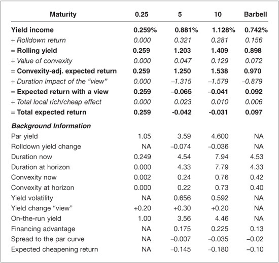
As a numerical illustration, Exhibit 37–5 shows the various expected-return measures for three bonds (the three-month Treasury bill and the five- and ten-year on-the-run Treasury notes) and for the barbell combination of the three-month bill and the ten-year bond. In this example we use as much market-based data as possible, for example, implied volatilities, not historical, to estimate the value of convexity and the “view” (rate predictions) based on survey evidence of the market’s rate expectations, not on a quantitative forecasting model. All the numbers are based on the market prices as of April 22, 2004.

EXHIBIT 37–5
Three-Month Expected Return Measures and Their Components, as of April 2004

NA, not available.
Note: Barbell is a combination of 0.56 unit of the ten-year par bond and 0.44 unit of the three-month bond; these weights duration-match the barbell with the five-year par bond bullet. Yield income is the return that a par bond earns over three months if it can be sold at its yield and if any cash-flows are reinvested at the yield. The yields are compounded semiannually and based on the Citigroup Treasury Model’s par yield-curve. Rolldown return is the capital gain that a bond earns from the rolldown yield change. Rolling yield is a bond’s horizon return given an unchanged yield-curve. Value of convexity is approximated by 0.5 × convexity at horizon × (yield volatility)² × (1 + rolling yield/100), where yield volatility is the basis-point yield volatility over a three-month horizon. The latter is computed by multiplying the on-the-run bond’s relative yield volatility—implied volatility based on the price of a three-month OTC option written on this bond—by its yield level and dividing by two (for deannualization). For the three-year bond, we interpolate between the implied volatilities of on-the-run twos and fives. Duration impact of the “view” is (− duration at horizon) × (expected change in a constant-maturity rate over the next three months) × (1 + rolling yield/100). In this example, the “view” reflects the market’s yield-curve expectations, broadly based on a Consensus Forecasts report. The “expected return with a view” measures the expected return for a hypothetical par bond that lies exactly on the model curve, ignoring any local cheapness or financing advantage of actual bonds. We can add to this four-term measure a fifth component called the total local rich/cheap effect. It is the sum of three additional sources of return for specific bonds: (1) the financing advantage (the difference between the three-month term repo rate for general collateral and the three-month special term repo rate for the on-the-run bond, divided by four for deannualization), (2) the spread between the on-the-run bond yield and the model par yield, divided by four for deannualization, and (3) the bond’s expected cheapening as it loses the richness associated with the on-the-run status.

The top panel of Exhibit 37–5 shows how nicely the different components of expected returns can be added to each other. Moreover, the barbell’s expected return measures are simply the market-value weighted averages of its components’ expected returns. In this case, the yield income, the rolldown return, and the value of convexity are all higher for the longer bonds. In contrast, the duration impact of the market’s rate view is negative because the consensus forecast indicates that the market expected rising rates over the next quarter. The local rich/cheap effect is marginally positive for the five- and ten-year notes; the reason is that the negative yield spread and the expected cheapening are not sufficient to offset the high repo market advantage. Based on “viewless” expected-return measures, the five-year bullet looks more attractive than the barbell, thanks to its carry and rolldown advantage. However, if we impose a consensus curve-flattening view (30 basis point rise in five-year rates versus 20 basis point rise in ten-year rates), the broad expected-return measures favor the barbell over the bullet.

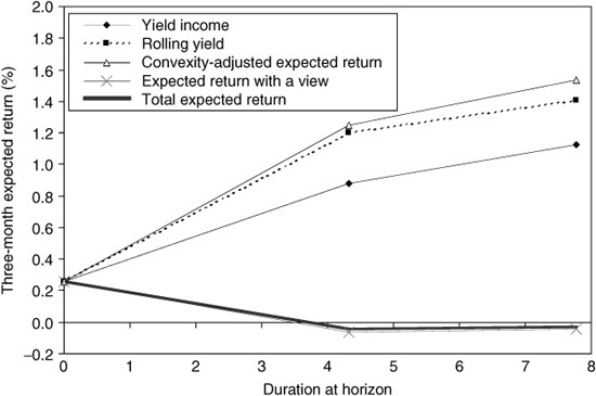
Exhibit 37–6 shows the five different expected-return curves plotted on the three bonds’ durations. In this case, the simplest expected-return measure (yield income) and the most comprehensive measure (total expected return) look very different, thanks to the strong bear-flattening view on yield-curve reshaping. In general, the relative importance of the five components may be dramatically different from that in Exhibit 37–5. The longer the asset’s duration and the shorter the investment horizon, the greater is the relative importance of the duration impact and the smaller is the impact of yield income. It is worth noting that realized returns can be decomposed in the same way as the expected returns and that the duration impact typically dominates the realized returns even more.¹⁴

EXHIBIT 37–6
Expected Returns of a Three-Month Bill, a Five-Year Bond, and a Ten-Year Bond, in April 2004

The total expected returns, if estimated carefully, should produce the most useful signals for relative-value analysis because they include all sources of expected returns. Yield spreads may be useful signals, but they are only a part of the picture. Therefore, we advocate the monitoring of broader expected-return measures relative to their history as cheapness indicators—just as yield spreads often are monitored relative to their history.

The components of expected returns just discussed are not new. However, few investors have combined these components into an integrated framework and based their historical analysis on broad expected-return measures. An additional useful feature of this framework is that all types of government bond trades can be evaluated consistently within it: the portfolio-duration decision (market-directional view), the maturity-sector positioning and barbell-bullet decision (curve-reshaping view), and the individual-issue selection (local cheapness view). With small modifications, the framework can be extended to include the cross-country analysis of currency-hedged government bond positions. Other possible future extensions include the analysis of foreign-exchange exposure and the analysis of spread positions between government bonds and other fixed income assets.

We finish with some reservations. Even if two investors use the same general framework and the same type of expected-return measure, they may come up with different numbers because of different data sources and different estimation techniques. The whole analysis can be made with any raw material; we emphasize the importance of good-quality inputs. Various candidates for the raw material include on-the-run and off-the-run government bonds, STRIPS, Eurodeposits, swaps, and Eurodeposit futures. [This multitude, of course, opens the possibility of trading between these curves if we can assess how various characteristics (say, convexity) are priced in each curve.] The most common approach is first to estimate the spot curve (or discount function) using a broad universe of coupon government bonds as the raw material and then to compute the forward rates and other relevant numbers. In European bond markets, the liquid swap curve (using cash Eurodeposits and swaps as the raw material) has gained more of a benchmark status. Of course, some credit and tax-related spread may exist between the swap curve and the government bond yield-curve. Recently, yet another approach has become popular: Eurodeposit futures prices are used as the raw material. In this case, the forward rates are computed by adjusting for the convexity difference between a futures contract and a forward contract, and only then are spot rates computed from the forwards. Some components of expected returns are easier to measure—and less debatable—than others. The yield income is relatively unambiguous. The rolldown return and the local rich/cheap effects depend on the curve-fitting technique. The value of convexity depends on the volatility input and thus on the volatility estimation technique. The rate “view,” the fourth term, can be based on various approaches, such as quantitative modeling or subjective forecasting, that rely on fundamental or technical analysis. Even the quantitative approach is not purely objective because infinitely many alternative forecasting models and estimation techniques exist. Forecasting rate changes is, of course, the most difficult task, as well as the one with greatest potential rewards and risks. Forecasting changes in yield spreads may be almost as difficult. The short-term returns of most bond positions depend primarily on the duration impact (rate changes or spread changes). However, even if investors cannot predict rate changes, they may earn superior returns in the long run—and with less volatility—by systematically exploiting the more stable sources of expected-return differentials across bonds: yields, rolldown returns, value of convexity, and local rich/cheap effects. More generally, while the total expected return differentials are, in theory, better relative-value indicators than the yield spreads, in practice, measurement errors conceivably can make them so noisy that they give worse signals. Therefore, it is important to check with historical data that any supposedly superior relative value tools would have enhanced the investment performance, at least in the past.

Link to Scenario Analysis

Many active investors base their investment decisions on subjective yield-curve views, often with the help of scenario analysis. Our framework for relative-value analysis is closely related to scenario analysis. It may be worthwhile to explore the linkages further.

An investor can perform the scenario analysis of noncallable government bonds in two steps. First, the investor specifies a few yield-curve scenarios for a given horizon and computes the total return of her bond portfolio—or perhaps just a particular trade—under each scenario. Second, the investor assigns subjective probabilities to the different scenarios and computes the probability-weighted expected return for her portfolio. Sometimes the second step is not completed, and investors only examine qualitatively the portfolio performance under each scenario. However, we advocate performing this step because investors can gain valuable insights from it. Specifically, the probability-weighted expected return is the “bottom line” number a total return manager should care about. By assigning probabilities to scenarios, investors also can explicitly back out their implied views about the yield-curve reshaping and about yield volatilities and correlations.

In scenario analysis, investors define the mean yield-curve view and the volatility view implicitly by choosing a set of scenarios and by assigning them probabilities. In contrast, our framework for relative-value analysis involves explicitly specifying one yield-curve view (which corresponds to the probability-weighted mean yield-curve scenario) and a volatility view (which corresponds to the dispersion of the yield-curve scenarios). Either way, the yield-curve view determines the duration impact, and the volatility view determines the value of convexity.

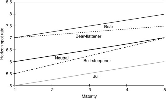
Exhibit 37–7 presents a portfolio that consists of five equally weighted zero-coupon bonds with maturities of one to five years and (annually compounded) yields between 6% and 7%. The portfolio’s maturity—and its Macaulay duration—initially is three. Over a one horizon, each zero’s maturity shortens by one year. We specify five alternative yield-curve scenarios over the horizon: parallel shifts of +100 basis points and −100 basis points, no change, a yield increase combined with a curve flattening, and a yield decline combined with a curve steepening (see Exhibit 37–8). We compute the one-year holding-period returns for each asset and for the portfolio under each scenario. In particular, the neutral scenario shows the rolling yield that each zero earns if the yield-curve remains unchanged. We can evaluate each scenario separately. However, such analysis gives us limited insight—for example, the last column in Exhibit 37–7 shows just that bearish scenarios produce lower portfolio returns than bullish scenarios.

EXHIBIT 37–7
Scenario Analysis and Expected Bond Returns

In contrast, if we assign probabilities to the scenarios, we can back out many numbers of potential interest. We begin with a simple example in which we use only the two first scenarios, parallel shifts of 100 basis points up or down. If we assign these scenarios equal probabilities (0.5), the expected return of the portfolio is 7.04% (= 0.5 × 5.02 + 0.5 × 9.06). On average, these scenarios have no view about curve changes, yet this expected return is 4 basis points higher than the expected portfolio return given no change in the curve (i.e., the 7% rolling yield computed in the neutral scenario). This difference reflects the value of convexity. If we use only one scenario, we implicitly assume zero volatility, which leads to downward-biased expected-return estimates for positively convex bond positions. If we use the two first scenarios (bear and bull), we implicitly assume a 100 basis point yield volatility; this assumption may or may not be reasonable, but it certainly is more reasonable than an assumption of no volatility. This example highlights the importance of using multiple scenarios to recognize the value of convexity. (The value is small here, however, because we focus on short-duration assets that have little convexity.)

Now we return to the example with all five yield-curve scenarios in Exhibit 37–8. As an illustration, we assign each scenario the same probability (p_i = 0.2). Then it is easy to compute the portfolio’s probability-weighted expected return:

EXHIBIT 37–8
Various Yield-Curve Scenarios

Given these probabilities, we can compute the expected return for each asset, and it is possible to back out the implied yield-curve views. The lower panel in Exhibit 37–7 shows that the mean yield change across scenarios is +10 basis points for each rate (because the bear-flattener and the bull-steepener scenarios are not quite symmetric in magnitude in this example), implying a mild bearish bias but no implied curve-steepness views. In addition, we can back out the implied basis point yield volatilities (or return volatilities) by measuring how much the yield-change (or return) outcomes in each scenario deviate from the mean. These yield volatility levels are important determinants of the value of convexity. The last line in Exhibit 37–7 shows that the volatilities range from 80 to 66 basis points, implying an inverted term structure of volatility. Finally, we can compute implied correlations between various maturity-yield changes; the curve behavior across the five scenarios is so similar that all correlations are 0.92 or higher (not shown). Note that all correlations would equal 1.00 if only the first three scenarios were used; the imperfect correlations arise from the bear-flattener and the bull-steepener scenarios.

Whenever an investor uses scenario analysis, he should back out these implicit curve views, volatilities, and correlations—and check that any biases are reasonable and consistent with his own views. Without assigning the probabilities to each scenario, this step cannot be completed; then the investor may overlook hidden biases in his analysis, such as a biased curve view or a very high or low implicit volatility assumption that makes positive convexity positions appear too good or too bad. If investors use quantitative tools—such as scenario analysis, mean-variance optimization, or the approach outlined in this chapter—to evaluate expected returns, they should recognize the importance of their rate views in this process. Strong subjective views can make any particular position appear attractive. Therefore, investors should have the discipline and the ability to be fully aware of the views that are input into the quantitative tool.

In addition to the implied curve views, we can back out the four components of expected returns discussed earlier. In this example, we only analyze bonds that lie “on the curve” and thus can ignore the fifth component, the local rich/cheap effects. First, we measure the yield income from the portfolio by a market-value weighted-average yield of the five zeros, which is 6.50%. Second, each asset’s rolldown return is the difference between the horizon return given an unchanged yield-curve and the yield income. Exhibit 37–7 shows that the horizon return for the portfolio is 7% in the neutral scenario; thus the portfolio’s (market-value weighted average) rolldown return is 50 basis points (= 7% – 6.5%). Note that the rolldown return is larger for longer bonds, reflecting the fact that the same roll-down yield change (25 basis points) produces larger capital gains for longer bonds. Third, the value of convexity for each zero can be approximated by 0.5 × convexity at horizon × (basis point yield volatility)² × (1 + rolling yield/100). Using the implicit yield volatilities in Exhibit 37–7, this value varies between 0.6 and 4.5 basis points across bonds. The portfolio’s value of convexity is a market-value weighted average of the bond-specific values of convexity, or roughly 2 basis points. Fourth, the duration impact of the rate “view” for each bond equals (– duration at horizon) × (expected yield change) × (1 + rolling yield/100). The last term is needed because each invested dollar grows to (1 + rolling yield/100) by the end of horizon when the repricing occurs. The core of the duration impact is the product of duration and expected yield change. The expected yield change refers to the change (over the investment horizon) in a constant-maturity rate of the bond’s horizon maturity. In Exhibit 37–7, all rates are expected to increase by 10 basis points, and the duration impact on specific bonds’ returns varies between 0 and –40 basis points. The portfolio’s duration impact is a market-value weighted average of bond-specific duration impacts, or about –20 basis points.

The four components add up to the total probability-weighted expected return of 6.82% (= 6.50% + 0.50% + 0.02% – 0.20%). Decomposing expected returns into these components should help investors to better understand their own investment positions. For example, they can see what part of the expected return reflects static market conditions and what part reflects their subjective market view. Unless they are extremely confident about their market view, they can emphasize the part of expected-return advantage that reflects static market conditions. In our example, the duration effect is small because the implied rate view is quite mild (10 basis points), and the one-year horizon is relatively long (the “slower” effects need time to accrue). With a shorter horizon and stronger rate views, the duration impact easily would dominate the other effects.

APPENDIX 37 A
Decomposing the Forward Rate Structure into Its Main Determinants

In this appendix we show how the forward rate structure is related to the market’s rate expectations, bond risk premia, and convexity bias. In particular, the holding-period return of an n-year zero-coupon bond can be described as a sum of its horizon return given an unchanged yield-curve and the end-of-horizon price change that is caused by a change in the n – 1 year constant-maturity spot rate (Δs_n−1). The horizon return equals a one-year forward rate, and the end-of-horizon price change can be approximated by duration and convexity effects. These relations are used to decompose near-term expected bond returns and the one-period forward rates into simple building blocks. All rates and returns used in the following equations are compounded annually and expressed in percentage terms.

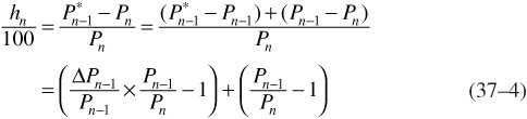
where h_n is the one-period holding-period return of an n-year bond, P_n is its price (today), is its price in the next period (when its maturity is n − 1), and ΔP_n−₁ = − P_n−₁. The second term on the right-hand side of Eq. (37–4) is the bond’s rolling yield (horizon return). The first term on the right-hand side of Eq. (37–4) is the instantaneous percentage price change of an n − 1 year zero multiplied by an adjustment term P_n−₁/P_n.¹⁵

Equation (37–5) shows that the zero’s rolling yield (P_n−1/P_n) equals, by construction, the one-year forward rate between n − 1 and n. Moreover, the adjustment term equals one plus the forward rate.

Equation (37–6) shows the well-known result that the percentage price change (ΔP/P) is closely approximated by the first two terms of a Taylor series expansion, duration and convexity effects.

where

Plugging Eqs. (37–5) and (37–6) into Eq. (37–4), we get

Even if the yield-curve shifts occur during the horizon, for performance calculation purposes, the repricing takes place at the end of horizon. This disparity causes various differences between the percentage price changes in Eqs. (37–6) and (37–7). First, the amount of capital that experiences the price change grows to (1 + f_n−₁,_n/100) by the end of horizon. Second, the relevant yield change is the change in the n – 1 year constant-maturity rate, not in the n-year zero’s own yield (the difference is the rolldown yield change).¹⁶ Third, the end-of-horizon (as opposed to the current) duration and convexity determine the price change.

The realized return can be split into an expected part and an unexpected part. Taking expectations of both sides of Eq. (37–7) gives us the n-year zero’s expected return over the next year:

Recall from Eq. (37–5) that the one-period forward rate equals a zero’s rolling yield, which can be split to yield and rolldown return components. In addition, the expected yield change squared is approximately equal to the variance of the yield change or the squared volatility E(Δs_n−₁)² ≈ [vol(Δ_n−1)]². This relation is exact if the expected yield change is zero. Thus the zero’s near-term expected return can be written (approximately) as a sum of the yield income, the rolldown return, the value of convexity, and the expected capital gains from the rate “view” (see Eq. 37–3).

We can interpret the expectations in Eq. (37–8) to refer to the market’s rate expectations. Mechanically, the forward rate structure and the market’s rate expectations on the right-hand side of Eq. (37–8) determine the near-term expected returns on the left-hand side. These expected returns should equal the required returns that the market demands for various bonds if the market’s expectations are internally consistent. These required returns, in turn, depend on factors such as each bond’s riskiness and the market’s risk-aversion level. Thus it is more appropriate to think that the market participants, in the aggregate, set the bond market prices to be such that given the forward rate structure and the consensus rate expectations, each bond is expected to earn its required return.¹⁷

Subtracting the one-period riskless rate (s₁) from both sides of Eq. (37–8), we get

We define the bond risk premium as BRP_n ≡ E (h_n s₁) and the forward-spot premium as FSP_n ≡ f_n−1,_n − s₁. The forward-spot premium measures the steepness of the one-year forward rate curve (the difference between each point on the forward rate curve and the first point on that curve), and it is closely related to simpler measures of yield-curve steepness. Rearranging Eq. (37–9), we obtain

In other words, the forward-spot premium is approximately equal to a sum of the bond risk premium, the impact of rate expectations (expected capital gain/loss caused by the market’s rate “view”), and the convexity bias (expected capital gain caused by the rate uncertainty). Unfortunately, none of the three components is directly observable.

The analysis thus far has been very general, based on accounting identities and approximations, not on economic assumptions. Various term-structure hypotheses and models differ in their assumptions. Certain simplifying assumptions lead to well-known hypotheses of the term-structure behavior by making some terms in Eq. (37–10) equal zero—although fully specified term-structure models require even more specific assumptions. First, if constant-maturity rates follow a random walk, the forward-spot premium mainly reflects the bond risk premium but also the convexity bias [E(Δs_n−₁) = 0 ⇒ FSP_n ≈ BRP_n + CB_n−₁]. Second, if the local-expectations hypothesis holds (all bonds have the same near-term expected return), the forward-spot premium mainly reflects the market’s rate expectations but also the convexity bias [BRP_n + 0 ⇒ FSP_n ≈ dur_n−1 E(Δs_n−1) + CB_n−₁]. Third, if the unbiased-expectations hypothesis holds, the forward-spot premium only reflects the market’s rate expectations [BRP_n + CB_n−₁ = 0 ⇒FSP_n ≈ dur_n−1E(Δs_n−₁)]. The last two cases illustrate the distinction between two versions of the pure expectations hypothesis.

APPENDIX 37 B
Relating Various Statements about Forward Rates to Each Other

We make several statements about forward rates—describing, interpreting, and decomposing them in various ways. The multitude of these statements may be confusing; therefore, we now try to clarify the relationships between them.

We refer to the spot curve and the forward curves on a given date as if they were unambiguous. In reality, different analysts can produce somewhat different estimates of the spot curve on a given date if they use different curve-fitting techniques or different underlying data (asset universe or pricing source). We acknowledge the importance of these issues—having good raw material is important to any kind of yield-curve analysis—but here we ignore these differences. We take the estimated spot curve as given and focus on showing how to interpret and use the information in this curve.

In contrast, the relations between various depictions of the term structure of interest rates (par, spot, and forward rate curves) are unambiguous. In particular, once a spot curve has been estimated, any forward rate can be computed mathematically by using Eq. (37–11):

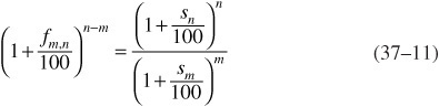
where f_m,n is the annualized n − m year interest rate m years forward and s_n and s_m are the annualized n-year and m-year spot rates, expressed in percent. Thus a one-to-one mapping exists between forward rates and current spot rates. The statement “the forwards imply rising rates” is equivalent to saying that “the spot curve is upward sloping,” and the statement “the forwards imply curve flattening” is equivalent to saying that “the spot curve is concave.” Moreover, an unambiguous mapping exists between various types of forward curves, such as the implied spot curve one year forward (f_1,n) and the curve of constant-maturity one-year forward rates (f_n−1,_n).

The forward rate can be the agreed interest rate on an explicitly traded contract, a loan between two future dates. More often the forward rate is defined implicitly from today’s spot curve based on Eq. (37–11). However, arbitrage forces ensure that even the explicitly traded forward rates would equal the implied forward rates and thus be consistent with Eq. (37–11). For example, the implied one-year spot rate four years forward (also called the one-year forward rate four years ahead, f_4,5) must be such that the equality (1 + s₅/100)⁵ = (1 + s₄/100)⁴(1 + f_4,5/100) holds. If f_4,5 is higher than this, arbitrageurs can earn profits by short selling the five-year zeros and buying the four-year zeros and the one-year forward contracts four years ahead, and vice versa. Such activity should make the equality hold within transaction costs.

Forward rates can be viewed in many ways: the arbitrage interpretation, the break-even interpretation, and the rolling yield interpretation. According to the arbitrage interpretation, implied forward rates are such rates that would ensure the absence of riskless arbitrage opportunities between spot contracts (zeros) and forward contracts if the latter were traded. According to the break-even interpretation of forward rates, implied forward rates are such future spot rates that would equate holding-period returns across bond positions. According to the rolling-yield interpretation, the one-period forward rates show the one-period horizon returns that various zeros earn if the yield-curve remains unchanged. Each interpretation is useful for a certain purpose: active view taking relative to the forwards (break-even), relative-value analysis given no yield-curve views (rolling yield), and valuation of derivatives (arbitrage).

All these interpretations hold by construction (from Eq. 37–11). Thus they are not inconsistent with each other. For example, the one-period forward rates can be interpreted and used in quite different ways. The implied one-year spot rate four years forward (f _4,5) can be viewed as either the break-even one-year rate four years into the future or the rolling yield of a five-year zero over the next year. Both interpretations follow from the equality (1 + s₅/100)⁵ = (1 + s₄/100)⁴(1 + f_4,5/100). This equation shows that the forward rate is the break-even one-year reinvestment rate that would equate the returns between two strategies (holding the five-year zero to maturity versus buying the four-year zero and reinvesting in the one-year zero when the four-year zero matures) over a five-year horizon. [Rewriting the equality as (1 + s₄/100)⁴ = (1 + s₅/100)⁵/(1 + f_4,5/100) gives a slightly different viewpoint; the forward rate also is the break-even selling rate that would equate the returns between two strategies (holding the four-year zero to maturity versus buying the five-year zero and selling it after four years as a one-year zero) over a four-year horizon.] Finally, rewriting the equality as 1 + f_4,5/100 = (1 + s₅/100)⁵/(1 + s₄/100)⁴ shows that the forward rate is the horizon return from buying a five-year zero at rate s₅ and selling it one year later as a four-year zero at rate s₄ (thus the constant-maturity four-year rate is unchanged from today). Our analysis focuses on the last (rolling-yield) interpretation.

Interpreting the one-period forward rates as rolling yields enhances our understanding about the relation between the curve of one-year forward rates (f_0,1, f_1,2, f_2,3, . . . , f_n−1,_n) and the implied spot curve one year forward (f _1,2, f_1,3, f_1,4, . . . , f_1,n). The latter “break-even” curve shows how much the spot curve needs to shift to cause capital gains/losses that exactly offset initial rolling-yield differentials across zeros and thereby equalize the holding-period returns. Thus a steeply upward-sloping curve of one-period forward rates requires, or “implies,” a large offsetting increase in the spot curve over the horizon, whereas a flat curve of one-period forward rates only implies a small “break-even” shift in the spot curve.¹⁸ A similar link exists for the rolling-yield differential between a duration-neutral barbell versus bullet and the break-even yield-spread change (curve-flattening) that is needed to offset the bullet’s rolling-yield advantage. These examples provide insight as to why an upward-sloping spot curve implies rising rates and why a concave spot curve implies a flattening curve.

Appendix 37A showed that forward rates can be decomposed conceptually into three main determinants (rate expectations, risk premia, and convexity bias). One might hope that the arbitrage, break-even, or rolling-yield interpretations could help us in backing out the relative roles of rate expectations, risk premia, and convexity bias in a given day’s forward rate structure. However, such hope is in vain. The three interpretations hold quite generally because of their mathematical nature. Thus they do not guide us in decomposing the forward rate structure.

Therefore, even when two analysts agree that today’s forward rate structure is an approximate sum of three components, they may disagree about the relative roles of these components. We can try to address this question empirically. It is closely related to the question about the forward rates’ ability to forecast future rate changes and future bond returns. Ignoring convexity bias, if the forwards primarily reflect rate expectations, they should be unbiased predictors of future spot rates (and they should tell little about future bond returns). However, if the forwards mainly reflect required bond risk premia, they should be unbiased predictors of future bond returns (and they should tell little about future rate changes).¹⁹,²⁰

Finally, our analysis does not reveal the fundamental economic determinants of the required risk premia or the market’s rate expectations—nor does it tell us to what extent the nominal rate expectations reflect expected inflation and expected real rates. Macroeconomic news about economic growth, inflation rates, budget deficits, and so on can influence both the required risk premia and the market’s rate expectations. More work clearly is needed to improve our understanding about the mechanisms of these influences.

KEY POINTS

• Yield-curve or forward rates can be decomposed into three main determinants: the market’s rate expectations, required bond risk premiums, and convexity bias.

• In an analogous fashion, the expected return of a position in a (default-free) bond—or in a long-short position across such bonds—can be decomposed into a few building blocks: the yield income and so-called rolldown return, the value of convexity, and the duration impact of a curve view.

• The first three components of the expected return amount to the reasonably predictable “viewless” part, while the last component is the least certain but dominates realized returns.

• The above decompositions provide a useful framework for analyzing the attractiveness of yield-curve trades. For analyzing the attractiveness of individual issues, the local richness of a bond relative to the curve and its richness in the repo market are important additional considerations.