
CHAPTER
THIRTY-NINE
TERM STRUCTURE MODELING WITH NO-ARBITRAGE INTEREST RATE MODELS
GERALD W. BUETOW, JR., PH.D., CFA
Chief Investment Officer
Innealta Capital
BRIAN J. HENDERSON, PH.D., CFA
Assistant Professor of Finance
The George Washington University
Interest rate models are important tools used by practitioners for purposes including pricing of fixed income securities, pricing interest rate contingent claims, and evaluation of interest rate risk. Although there are many interest rate models, the models vary by their assumptions regarding interest rate dynamics and their degree of specificity. Due to differing assumptions about the interest rate process, each model has different properties that have important implications for their use in valuation. The models range from fairly simplistic to highly mathematical and complex, reflecting the tradeoff between analytical tractability and how closely the model captures interest rate dynamics.
The focus in this chapter is on no-arbitrage interest rate models. This term means that the models are fit to the current term structure so that valuing bonds with the model results in prices that are consistent with market prices. In addition to no-arbitrage models, another class of interest rate models called equilibrium models, begin with a stochastic differential process and develop pricing mechanisms under a general equilibrium framework. Our focus on no-arbitrage models stems from the fact that these models seem to be the most widely accepted among practitioners.
In general, interest rate models begin with a stochastic differential equation (SDE) to describe the dynamics of an interest rate. One-factor models represent the short rate of interest, whereas multifactor models incorporate a SDE for additional interest rates. Obtaining closed-form solutions to interest rate models requires the use of stochastic calculus. Instead of assuming the reader is versed in stochastic calculus, we present the models in the most tractable way possible.
In this chapter, we illustrate several no-arbitrage interest rate models. Our presentation focuses on the important characteristics of each model with an emphasis on the key assumptions driving the models and the properties of the models that reflect these assumptions. Although more sophisticated models exist, the models presented in this chapter are built on the same intuition and algebraic properties as more sophisticated models.
For interest rate models to be useful for practical purposes, it is helpful to adapt them to a recombining lattice structure. This usually translates into binomial or trinomial trees. After presenting the models and highlighting their important properties, we illustrate the models using lattices. The lattice approach is a useful tool for pricing interest rate contingent claims such as callable bonds and swaptions and for evaluating interest rate risk exposure.
INTRODUCTION TO MODELS OF THE SHORT RATE
We present five no-arbitrage models of the short rate in this section. Our focus is on the assumptions behind each of the models and the implications of those assumptions on the resulting rate scenarios. In the next section we build on these ideas by presenting the models fit to binomial lattices to illustrate the important properties.
Ho-Lee Model
The first no-arbitrage interest rate model was that of Ho and Lee.1 The model assumes that the short-rate follows the stochastic process:
![]()
This continuous-time process expresses the short-rate dynamics as a combination of an expected component and a random shock. The term θ(t)dt is the expected change component that is also referred to as the drift in the short rate. This component is the source of important characteristics, such as mean reversion, driving the expected change in interest rates. The drift parameter is a function of time and its value comes from the current term-structure through the process of fitting the model to the no-arbitrage constraints, which we will illustrate below.
The second component in the continuous time process is the source of risk and is the product of σ and dz. This component is important since it drives the distributional characteristics of the interest rate. The Ho-Lee interest rate model assumes the level of risk is constant through time and is referred to as a normal process since z is a Weiner process that is distributed normally. The term ![]() is distributed normally since ε comes from a standard normal distribution with zero mean and unit standard deviation. Thus, the Ho-Lee process models the short rate as normally distributed. As we will see shortly, this means that negative interest rates are possible in the model.
is distributed normally since ε comes from a standard normal distribution with zero mean and unit standard deviation. Thus, the Ho-Lee process models the short rate as normally distributed. As we will see shortly, this means that negative interest rates are possible in the model.
We develop a discrete numerical approximation to generate approximate interest rates. Denoting the exact solution to the stochastic differential equation at time tk as r(tk), the numerical algorithm generates solutions denoted rk that approximate the exact solutions r(tk). For very small discrete time steps, where Δt is close to zero, we have dt ≈ Δt = tk+1 − tk. This leads to an approximation for the interest rate where dr ≈ Δr = r(tk+1) − r(tk) ≈ rk+1 − rk. Using the discrete approximation, we are able to write the approximation for the Ho-Lee model for the interest rate movement from time k to k+ 1 as:
![]()
where tk = kτ, and Δzk is a numerical (discrete) approximation of dz. Substituting ![]() , the equation becomes:
, the equation becomes:
![]()
where εk is a random number drawn from the standard normal distribution N(0,1). We denote the time step between time tk and the starting point as τ. Examining the above equation, it is clear that the short rate’s mean may grow very large over time; this happens for certain θ where θkτ can become large. Additionally, it is clear that for large volatility shocks, the short rate dynamics can be heavily influenced by volatility and the random shock component may be very large. Thus, there are two primary shortcomings of the Ho and Lee model: The interest rate can exhibit uncontrolled growth and negative interest rates are possible.
Hull-White Model
The stochastic process for the Hull-White interest rate model is2:
![]()
The process in (39.4) is similar to the Ho-Lee process in (39.1) in that the volatility is assumed to be constant through time and the rates are distributed normally. Additionally, negative interest rates are possible in the Hull-White model. The drift term in the Hull-White process differs from Ho-Lee process. Note that if θ equals zero, then the Hull-White model reduces to the Ho-Lee model. The drift term in the Hull-White model captures the mean-reversion property of interest rates and is an attempt to control the uncontrolled growth of the short rate that is possible in the Ho-Lee model.
If we define the long run target short rate as μ = θ/ϕ, then we can rearrange the drift term in equation (39.4) to be ϕ(μ − r). When the short-rate is below the target rate μ, then in future periods the rate drifts upwards toward that target rate. Conversely, in periods when the short rate is greater than the target rate, the drift term pulls future rates back toward the target rate. The parameter ϕ controls the speed of mean-reversion. If ϕ is close to zero, the speed at which the short rate tends toward the target rate is slower than cases in which ϕ is close to one. Positive mean-reversion occurs when ϕ takes a positive value. Negative mean reversion is possible when ϕ takes a negative value, but results in exponential growth in the short rate through time. Another important feature of mean-reversion is that the drift toward the target rate is determined partially by how far the short rate is from the target rate, the drift being larger when the short rate is further from the target. In the case of negative mean-reversion, this second effect amplifies the exponential growth of the short rate.
Applying the discrete approximation for the Hull-White stochastic process, as described for the Ho-Lee model, we obtain the following approximation:
![]()
The numerical approximation for the Hull-White process, like the Ho-Lee process, models the short rate as normally distributed. The normality assumption is evident since εk is a random number drawn from the standard normal distribution N (0,1). Additionally, it is clear that short rates can become negative, particularly when the assumed level of volatility is large.
Due to the additional parameters of the model, the algebra required to fit the Hull-White process to the lattice involves a variable time step. The variable time step is an undesirable property, requiring a spline methodology to engineer equal time steps. Using a trinomial lattice instead of a binomial lattice will introduce an additional degree of freedom allowing the solutions to have fixed time steps between nodes. Thus, when we present the model lattices, we will present the trinomial model for the Hull-White model.
Kalotay-Williams-Fabozzi Model
The Kalotay-Williams-Fabozzi (KWF) model is analogous to the Ho-Lee model as the stochastic process has a constant drift, does not include mean-reversion, and exhibits constant volatility.3 However, the incremental distinction is that the model treats the natural logarithm of the interest rate as normally distributed. Although the natural logarithm of the short rate may be negative, the short rate itself does not turn negative in this model, unlike the Ho-Lee and Hull-White models. Specifically, the differential process for the KWF model is:
![]()
We can see that this equation is identical to the Ho-Lee model if μ = ln(r) and we re-write the process as:
![]()
Since μ follows a normal process, ln(r) follows a normal process, implying that r follows a lognormal process. Although μ may become negative as in the Ho-Lee and Hull-White processes, r may not become negative. To illustrate, note that since μ = ln(r) then r = eμ which shows that r is always positive and the KWF model circumvents one of the problems from the Ho-Lee and Hull-White models, namely negative interest rates.
The discrete form approximation for the KWF model is:
![]()
Since μ = ln(r) we re-write the equation as:
![]()
From this equation, we see that when θ is positive, the short rate grows through time and is unbounded. Similarly, if θ is negative, the short rate decays toward zero. Like the Ho-Lee model, short rates in the KWF model exhibit potential unbounded growth, but the KWF model circumvents the negative short rates plaguing the Ho-Lee and Hull-White models. Additionally, the short rate is distributed log normally as opposed to normally.
Black-Karasinski Model
The interest rate process in the Black-Karasinski model takes the following form4:
![]()
If we again let μ = ln(r) and re-write the process, we obtain:
![]()
Note that this expression is the Hull-White interest rate process, and that since μ has those same properties as the rate in the Hull-White model, it is distributed normally and r is distributed log normally. Since r = eμ, the interest rate in the Black-Karasinski process is greater than zero, which is the advantage of this model over the Hull-White model.
Compared with the Kalotay-Williams-Fabozzi model, the Black-Karasinski model also includes mean-reversion of the interest rate. Similar to the Hull-White model’s extension of the Ho-Lee model, the Black-Karasinski model is an extension of the log normal KWF model to incorporate the mean-reversion property of interest rates. Similar to the Hull-White model, the parameter ϕ controls the growth of the short rate. The drift in the short term rate from each period to the next is determined by the speed of mean-reversion parameter and the distance of the rate from the target rate.
Next, we discretize the process using the same approach illustrated above for the other models:
![]()
Since μ = ln(r) we re-write the equation as:
![]()
Note the similarity of these equations and Equation (39.5) for the Hull-White model. Both models incorporate mean-reversion in the drift term but the main difference comes from the distributional assumption since the Hull-White is normal and Black-Karasinski is lognormal.
Black-Derman-Toy Model
Similar to the Black-Karasinski model, the Black-Derman-Toy (BDT) interest rate model combines mean-reversion and the lognormal distribution of the short rate.5 The important incremental contribution is that in the BDT model, mean reversion is determined endogenously, which is to say that it is determined based on the model’s input parameters. The mathematics behind this model make it the most complicated of the models we present. The short rate in the model follows the following process:
![]()
If we again let μ = ln(r) and re-write the process, we obtain:
![]()
Equation (39.15) is strikingly similar to the Black and Karasinski model in Equation (39.11), and the only difference between the two comes from the mean reversion parameter. In this model, mean reversion is endogenous to the model since it is determined by the assumed volatility of the short rate. The mechanics of mean reversion in this model should be similar, where the short rate is mean reverting when the term σ′(t) is less than zero. Conversely, when σ′(t) is positive, implying σ(t) is increasing, the short rate grows without mean reverting. Note that if the volatility is constant, the derivative is zero and the mean-reversion term is zero. In the case of constant volatility, the KWF model is a special case of the BDT model.
Next, we discretize the BDT interest rate process using the same approach as for the other models:
![]()
Since μ = ln(r) we re-write the equation as:
![]()
BINOMIAL INTEREST RATE LATTICES
In this section, we present binomial lattice representations of the interest rate models. In the binomial lattice, the interest rate may make one of two possible moves over discrete points in time. For our purposes, we present lattices where the length of each time step is six months. Exhibit 39–1 illustrates a four-period binomial tree. Note that at each node the interest rate takes either an up-step or a down-step. The size of each step is determined by the properties of the interest rate model. Additionally, notice that the tree recombines, meaning that an up-step followed by a down-step produces the same rate as a down-step followed by an up-step. Recombination is a common assumption in binomial trees and results from the imposition of additional algebraic constraints. The numerical methods required to fit the interest rate models to binomial trees are beyond the scope of this chapter, but we present binomial lattice representations of the model to illustrate the important features of the interest rate models. Buetow and Sochacki present a thorough discussion of the numerical methodologies involved with fitting the models to binomial trees.6
EXHIBIT 39–1
The Binomial Lattice of Forward Rates

The no-arbitrage property of the term structure models presented in this chapter comes from the fact that the model rates match the properties of the current term structure. For example, denoting the current one-period (six-month) spot rate as r1,0, the two-period spot rate as z, and the implied forward rate as ϕ1, we can illustrate the no-arbitrage property using the binomial lattice. The two possible values for the interest rate next period in the binomial lattice are r1,1 and r2,1, and the no-arbitrage property is satisfied by the following constraint, which requires the one period spot rate, followed by the one-period rate at the next time step, r1,1 or r2,1, to be equal to the two-period spot rate:
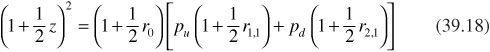
where pu and pd are the probabilities of the up and down move, respectively. Imposing the no-arbitrage constraint ensures that pricing straight bonds using the interest rate lattice generates prices that are consistent with the observed spot curve produced from market prices. Due to this property, the no-arbitrage models have practical appeal and are useful for pricing and risk-management purposes.
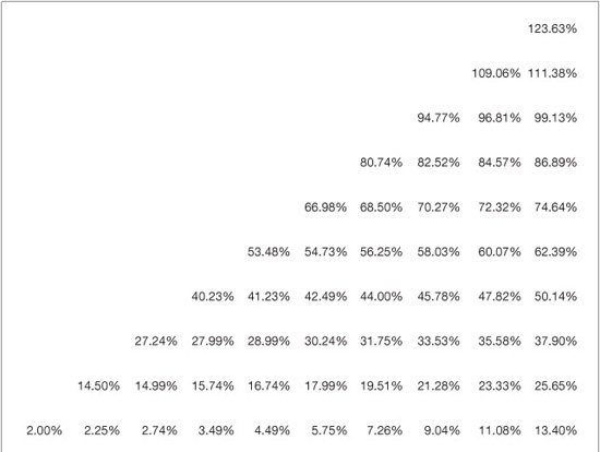
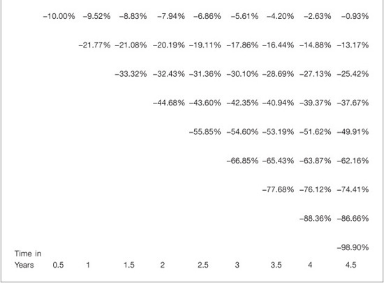
Exhibit 39–2 presents the Ho-Lee binomial lattice where the term structure is flat at 2% and volatility is constant. In Panel A of the exhibit, volatility is 1% and in Panel B, volatility is 10%. There are several important features of the Ho-Lee model evident in the binomial lattices. First, the one-period interest rate may be negative, which results from the fact that in the Ho-Lee process, the rate is distributed normally and is unbounded. In fact, it can be demonstrated that the spread between the high and low rates in the Ho-Lee lattice equals ![]() , where k is time (in years) and t is the length of the time step. This algebraic relation demonstrates that the spread, or distance, between the highest possible rate and the lowest at each time step is an increasing function of time and often produces negative rates. Additionally, the level of volatility drives the spread. To illustrate, panel B of Exhibit 39–2 presents the Ho-Lee lattice where volatility is 10%. The greater dispersion of rates resulting from the greater volatility is immediately evident and illustrates that rates in this model may be very large and frequently negative. Despite the undesirable economic interpretation of negative rates, they are not detrimental to the model since bond prices computed from the binomial trees are the average over the possible future short paths, averaging across all rates.
, where k is time (in years) and t is the length of the time step. This algebraic relation demonstrates that the spread, or distance, between the highest possible rate and the lowest at each time step is an increasing function of time and often produces negative rates. Additionally, the level of volatility drives the spread. To illustrate, panel B of Exhibit 39–2 presents the Ho-Lee lattice where volatility is 10%. The greater dispersion of rates resulting from the greater volatility is immediately evident and illustrates that rates in this model may be very large and frequently negative. Despite the undesirable economic interpretation of negative rates, they are not detrimental to the model since bond prices computed from the binomial trees are the average over the possible future short paths, averaging across all rates.
EXHIBIT 39–2
The Ho-Lee Binomial Interest Rate Lattice
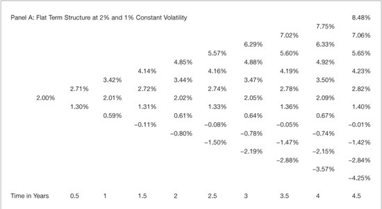

The Ho-Lee process models the short rate as distributed normally. This is evident in the binomial lattice representation since the rates are symmetrical around the mean rate. For example, the distance between rates r1,2 and r2,2 is identical to the distance between r2,2 and r3,2.
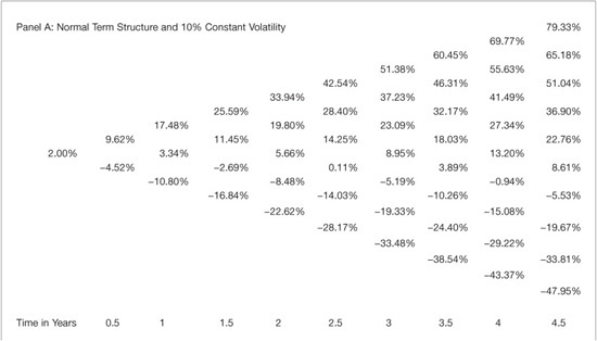
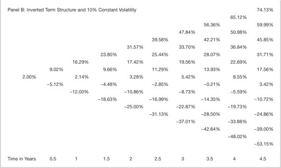
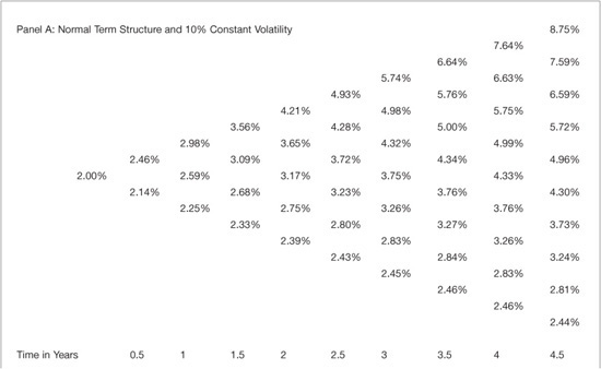
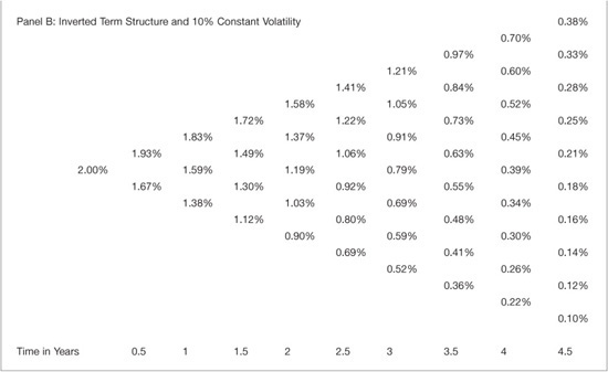
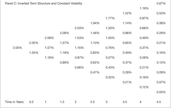
Another important property of the Ho-Lee model is that the drift term is related to the slope of the current term structure. This property is illustrated in panel A of Exhibit 39–3 where the term structure slopes upward and the forward curve is increasing by 15 basis points each period and volatility is constant at 10%. This example corresponds to a “normal” term structure since it is positively sloped. The positive drift term is evident and we note that the spread or dispersion between the nodes is identical to that in Panel B of Exhibit 39–2. The difference comes from the positive drift term. In some cases, since the drift is proportional to time and grows unboundedly, this term can become quite large. Correspondingly, when the drift term is positive, there are fewer negative interest rates in the lattice. Panel B of Exhibit 39–3 presents the Ho-Lee model for an inverted term structure where the forward curve decreases by 15 basis points each period and volatility is again 10%. Again, the spread between the highest and lowest rate is identical since the volatility is 10% and volatility drives the spread in the Ho-Lee model. Additionally, we can see that the drift term is negative and all rates in the Ho-Lee model shift down by that negative drift term compared with the flat or normal term structure scenarios.
EXHIBIT 39–3
Ho-Lee Binomial Lattice under Normal and Inverted Term Structures
We now turn to the KWF binomial lattice. Recall that this model is analogous to a log-normal version of the Ho-Lee model. It is also a special case of the BDT model when volatility is assumed to be positive and constant. Panel A of Exhibit 39–4 presents the KWT binomial lattice for the scenario where the term structure is flat at 2% and volatility is a constant 10%. This scenario is directly comparable to the scenario is Exhibit 39–2 panel B for the Ho-Lee model and there are two important distinctions between the two lattices. First, the log-normal distribution in the KWT model restrains the interest rate paths from becoming negative. Since the Ho-Lee model is distributed normally, negative rates are possible, but the log-normal distribution of the KWT model restricts rates to be positive. Second, the spread of possible rates at the same volatility level are smaller than in the Ho-Lee model. Whereas the rates are distributed normally around the center nodes in the Ho-Lee model, in the KWT model the rates are distributed asymmetrically around the center node and are skewed toward higher rates. This property illustrates the importance of the distributional assumptions stemming from the models’ differential processes.
EXHIBIT 39–4
The Kalotay-Williams-Fabozzi Binomial Interest Rate Lattice
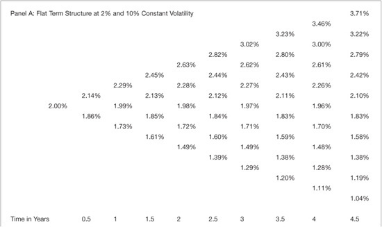
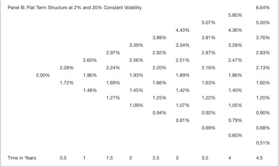
Exhibit 39–5 presents the KWT lattices for two additional scenarios to cover a normal term structure and an inverted term structure. Panel A presents the normal term structure scenario in which rates are increasing at 15 basis points per period and volatility is constant at 10%. Note that the rates grow larger over time which is the impact of the drift term. Panel B presents the lattice for the inverted term structure scenario in which the rates decrease by 10 basis points per period and volatility is again constant at 10%. Note that the rates grow smaller over time, illustrating the impact of negative drift under the inverted term structure. Additionally, we notice that the spread from the highest to the lowest rate on the lattice at each time step is noticeably smaller for the inverted term structure scenario than for the normal term structure. This observation is in stark contrast to the Ho-Lee model in which the spread is determined solely by volatility.
EXHIBIT 39–5
Kalotay-Williams-Fabozzi Binomial Lattice; Normal and Inverted Term Structures
Next, we turn to the BDT binomial lattice. Recall that the differential process in this model is lognormal and incorporates endogenous mean-reversion in which the slope of the volatility curve drives mean reversion in the model. Exhibit 39–6 presents the binomial lattice for the normal interest rate tree scenario where the current rate is 2% and the rate increases by 0.15 basis points each period. Panels A, B, and C present three scenarios for a normal term structure across different volatility structures. In Panel A, the volatility structure is decreasing from 20% by 0.5% each period, in Panel B it is increasing from 20% by 0.5% each period, and in Panel C it is constant. When volatility is constant, the model reduces to the KWT model. Note that the rates are all positive and are not extreme as in the normally distributed Ho-Lee model.
The shape of the volatility curve drives the model’s mean reversion. This is evident in Panels A, B, and C of Exhibit 39–6 since the only change across the panels is the shape of the volatility structure. Comparing Panel A to Panel C, it is clear that the decreasing volatility structure has the effect of increasing mean-reversion. Note that the upward drift and the spread from high to low rates at each time step are different. The upward drift is checked by the mean reversion when the volatility structure is decreasing and similarly the spread is lower. Comparing panel B to panel C, it is clear that under the positively sloped volatility structure, the upward drift is larger and the spread at each time step is greater.
EXHIBIT 39–6
Black-Derman-Toy Binomial Lattice: Normal Term Structure and Varying Volatility Structures
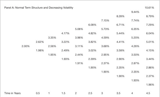


Exhibit 39–7 presents the BDT interest rate lattices for an inverted term structure where the current short rate is 2% and decreases by 10 basis points each period. The pattern that emerges is similar to the previous exhibit. Comparing panel A to panels B and C, it is clear that the mean-reversion from the decreasing volatility structure has the effect of reducing the spread across rates at each time step.
EXHIBIT 39–7
Black-Derman-Toy Binomial Lattice: Inverted Term Structure and Varying Volatility Structures


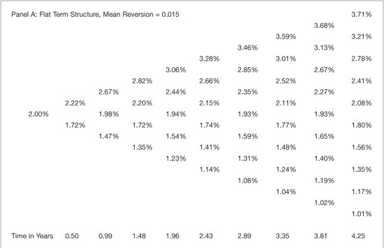
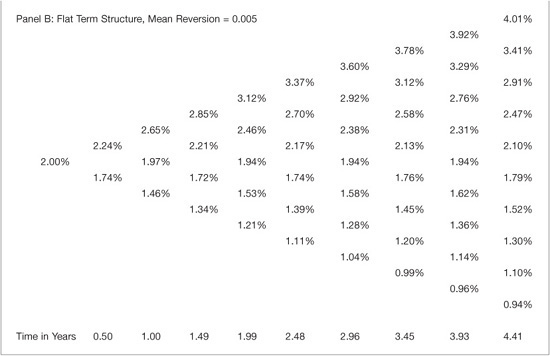
Turning to the Black-Karasinski model, Exhibit 39–8 presents the interest rate lattice for this model for a flat term structure of rates when volatility is initially 20% but decreases by 0.5% each period. To illustrate the importance of mean reversion in this model, the table contains two panels; Panel A illustrates the lattice with the mean-reversion parameter equal to 0.015 and Panel B illustrates the lattice when the mean-reversion parameter equals 0.005. The figures illustrate that larger mean reversion impacts the rates by narrowing the spread between the rates at each time step. Additionally, it must be noted that in order to fit the model to a binomial lattice the time-step must be allowed to vary for this model. Interpolation is necessary to adjust this tree to equally spaced time steps. The larger mean reversion leads to a decreasing time step. One way to circumvent the uneven time step in this model is to use a trinomial lattice since it allows for an extra degree of freedom.
EXHIBIT 39–8
Black-Karasinski Binomial Lattice: Inverted Term Structure
TRINOMIAL LATTICE
Turning to the Hull-White model, Exhibit 39–9 presents the Hull-White trinomial lattice. The trinomial structure is identical the binomial lattice except there are three possible time steps from each node instead of two. Similar to the binomial lattice, the solutions impose restrictions to ensure that the trinomial lattice recombines and that the rates in the tree satisfy the necessary conditions. Exhibit 39–9 presents the Hull-White trinomial lattice when the term structure is flat at 2%, 10% constant volatility, and zero mean reversion. The important properties of the Hull-White process are evident in the lattice: Interest rates become negative for the bottom nodes, the spread between high and low rates at each time step is large, and the rates are distributed normally. Additionally, an upward drift is evident in the middle nodes.
EXHIBIT 39–9
Hull-White Trinomial Lattice: Flat Term Structure, 10% Volatility, No Mean Reversion

Since the Hull-White model incorporates mean reversion, Exhibit 39–10 presents the Hull-White model with the same term structure and volatility as Exhibit 39–9, but incorporates 5% mean reversion. We expect the mean reversion will have the effect of pulling rates back toward the mean, or that the lattice tree should be “pruned.” The mean-reversion property is evident as the spread at each time step is reduced and each rate is pulled back toward the target rate, compared to the tree in Exhibit 39–9.
EXHIBIT 39–10
Hull-White Trinomial Lattice: Flat Term Structure, 10% Volatility, 5% Mean Reversion

In summary, the lattice representations of the no-arbitrage interest rate models discussed in this chapter demonstrate the importance of the model assumptions about the short-rate process on the model output. It is of critical importance that users of these models understand the model assumptions and the impact those assumptions have on any results (pricing or risk metrics) based on model outputs.
KEY POINTS
• Interest rate models are important tools for practitioners and are useful for pricing fixed income securities, valuing interest-rate contingent claims, and for risk management purposes.
• There exist many interest rate models. One factor models of the short rate make important assumptions about its dynamics through time. Understanding these assumptions and their implications is critical for practitioners.
• Interest rate models specify a stochastic differential equation to capture the dynamics of the models.
• Early models (Ho-Lee and Hull-White) assume the short rate is distributed normally. Interest rates in those models may be negative. Other models (Kalotay-Williams-Fabozzi, Black-Derman-Toy, and Black-Karasinski models) assume the short rate is distributed log-normally, restricting the short rate to be positive.
• Mean-reversion is the tendency for interest rates to tend toward a long-term target rate. Absent mean-reversion, an interest rate model may allow the short rate to grow unbounded.
• The no-arbitrage models incorporate the information in the current term structure and produce identical prices for option-free bonds.
• When pricing bonds with embedded option features, the interest rate model assumptions are critically important and may result in meaningful differences across different models.