CHAPTER
FORTY-ONE
VALUATION OF AGENCY MORTGAGE-BACKED SECURITIES

FRANK J. FABOZZI, PH.D., CFA, CPA

Professor of Finance
EDHEC Business School

SCOTT F. RICHARD, DBA

Practice Professor of Finance
Wharton
University of Pennsylvania

PETER RU

Director, Fixed Income Investment Department
Morgan Stanley Huaxin Fund Management Company Limited

The traditional approach to the valuation of fixed income securities is to calculate yield—the yield-to-maturity, the yield-to-call for a callable bond, and the cash-flow yield for a mortgage-backed security. A superior approach is the option-adjusted spread (OAS) method. Our objective in this chapter is to describe the OAS method as applied to mortgage-backed securities. At the end of the chapter, we apply the method to two agency collateralized mortgage obligation (CMO) deals.

In this chapter we describe the theoretical foundations of this technique, the input and assumptions that go into the development of an OAS model, and the output of an OAS model, which in addition to the OAS value includes the option-adjusted duration and option-adjusted convexity. Because the user of an OAS model is exposed to modeling risk, it is necessary to test the sensitivity of these numbers to changes in the assumptions.

Valuation modeling for CMOs is similar to valuation modeling for pass-throughs, although the difficulties are amplified because the issuer has sliced and diced both the prepayment risk and the interest-rate risk into smaller pieces called tranches. The sensitivity of the pass-through securities from which the CMO is created to these two risks is not transmitted equally to every tranche. Some of the tranches wind up more sensitive to prepayment risk and interest-rate risk than the collateral, whereas some of them are much less sensitive.

The objective of the money manager is to figure out how the OAS of the collateral or, equivalently, the value of the collateral gets transmitted to the CMO tranches. More specifically, the objective is to find out where the value goes and where the risk goes so that the money manager can identify the tranches with low risk and high value: the ones he wants to buy. The good news is that this combination usually exists in every deal. The bad news is that in every deal there are usually tranches with low OAS, low value, and high risk.

STATIC VALUATION

Using OAS to value mortgages is a dynamic technique in that many scenarios for future interest rates are analyzed. Static valuation analyzes only a single-interest-rate scenario, usually assuming that the yield-curve remains unchanged. Static valuation results in two measures, average life and static spread, which we review below.

Average Life

The average life of a mortgage-backed security is the weighted average time to receipt of principal payments (scheduled payments and projected prepayments). The formula for the average life is

where T is the number of months.

In order to calculate average life, an investor must either assume a prepayment rate for the mortgage security being analyzed or use a prepayment model. By calculating the average life at various prepayment rates, the investor can gain some feeling for the stability of the security’s cash-flows. For example, a PAC bond’s average life will not change within the PAC bands but may shorten significantly if the prepayment rate exceeds the upper band. By examining the average life at prepayment rates greater than the upper band, an investor can judge some of the PAC’s risks. With a prepayment model available, the average life of a mortgage security can be calculated by changing the mortgage refinancing rate. As the refinancing rate rises, the prepayment model will slow the prepayment rate and thus cause the bond’s average life to extend. Conversely, if the refinancing rate is lowered, the model will cause prepayments to rise and shorten the average life.

Static Spread

One of the standard measures in evaluating any mortgage-backed security is the cash-flow yield, or simply “yield.” The yield spread, sometimes called the nominal spread, is found by spreading the yield to the average life on the interpolated swap yield-curve. This practice is improper for an amortizing bond even in the absence of interest-rate volatility. Note that since late 1998, structured products are using swaps instead of Treasuries for pricing and hedging purposes. The main reason is that spread to swaps is more stable than to Treasuries.

What should be done instead is to calculate what is called the static spread. This is the yield spread in a static scenario (i.e., no volatility of interest rates) of the bond over the entire theoretical swap spot-rate curve, not a single point on the swap yield-curve. The magnitude of the difference between the nominal spread and the static yield depends on the steepness of the yield-curve: The steeper the curve, the greater the difference between the two values. In a relatively flat interest-rate environment, the difference between the nominal spread and the static spread will be small.

There are two ways to compute the static spread. One way is to use today’s yield-curve to discount future cash-flows and keep the mortgage refinancing rate fixed at today’s mortgage rate. Since the mortgage refinancing rate is fixed, the investor usually can specify a reasonable prepayment rate for the life of the security. Using this prepayment rate, the bond’s future cash-flow can be estimated. Use of this approach to calculate the static spread recognizes different prices today of dollars to be delivered at future dates. This results in the proper discounting of cash-flows while keeping the mortgage rate fixed. Effectively, today’s prices indicate what the future discount rates will be, but the best estimates of future rates are today’s rates.

The second way to calculate the static spread allows the mortgage rate to go up the curve as implied by the forward interest rates. This procedure is sometimes called the zero-volatility OAS. In this case, a prepayment model is needed to determine the vector of future prepayment rates implied by the vector of future refinancing rates. A money manager using static spread should determine which approach is used in the calculation.

DYNAMIC VALUATION MODELING

Because CMOs are simply a regrouping of the cash-flows from the underlying pass-through securities, the valuation of CMO tranches follows directly from the valuation of pass-through securities.

Using Simulation to Generate Interest-Rate Paths and Cash-Flows

A technique known as simulation is used to value complex securities such as mortgage-backed securities. Simulation is used because the monthly cash-flows are path-dependent. This means that the cash-flows received this month are determined not only by the current and future interest-rate levels but also by the path that interest rates took to get to the current level.

There are typically two sources of path dependency in a CMO tranche’s cash-flows. First, collateral prepayments are path-dependent because this month’s prepayment rate depends on whether there have been prior opportunities to refinance since the underlying mortgages were issued. Second, the cash-flow to be received this month by a CMO tranche depends on the outstanding balances of the other tranches in the deal. We need the history of prepayments to calculate these balances.

Conceptually, the valuation of pass-through securities using the simulation method is simple. In practice, however, it is very complex. The simulation involves generating a set of cash-flows based on simulated future mortgage refinancing rates, which, in turn, imply simulated prepayment rates.

The typical model that Wall Street firms and commercial vendors use to generate these random interest-rate paths takes as input today’s term structure of interest rates and a volatility assumption. The term structure of interest rates is the theoretical spot-rate (or zero-coupon) curve implied by today’s swap rates. The volatility assumption determines the dispersion of future interest rates in the simulation. The simulations should be normalized so that the average simulated price of a zero-coupon swap equals today’s actual price.

Each OAS model has its own model of the evolution of future interest rates and its own volatility assumptions. Until recently, there have been few significant differences in the interest-rate models of dealer firms and OAS vendors, although their volatility assumptions can be significantly different. Note that the volatility in term structure models is calibrated to the prices of liquid securities that reflect at-the-money options on interest rates, such as at-the-money caps and swaptions, as well as off-the-money swaptions (to capture the volatility skew).

The random paths of interest rates should be generated from an arbitrage-free model of the future term structure of interest rates. By arbitrage-free it is meant that the model replicates today’s term structure of interest rates, an input of the model, and that for all future dates there is no possible arbitrage within the model.¹

The simulation works by generating many scenarios of future interest-rate paths. In each month of the scenario, a monthly interest rate and a mortgage refinancing rate are generated. The monthly interest rates are used to discount the projected cash-flows in the scenario. The mortgage refinancing rate is needed to determine the cash-flow because it represents the opportunity cost the mortgagor is facing at that time.

If the refinancing rates are high relative to the mortgagor’s original coupon rate, the mortgagor will have less incentive to refinance or even a disincentive (i.e., the homeowner will avoid moving in order to avoid refinancing). If the refinancing rate is low relative to the mortgagor’s original coupon rate, the mortgagor has an incentive to refinance.

Prepayments are projected by feeding the refinancing rate and loan characteristics, such as age, into a prepayment model. Given the projected prepayments, the cash-flow along an interest-rate path can be determined.

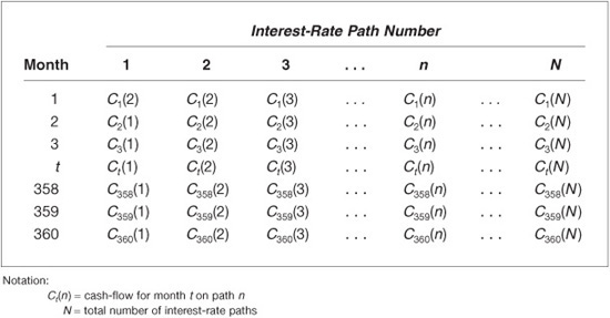
To make this more concrete, consider a newly issued mortgage pass-through security with a maturity of 360 months. Exhibit 41–1 shows N simulated interest-rate path scenarios. Each scenario consists of a path of 360 simulated one-month future interest rates. Just how many paths should be generated is explained later. Exhibit 41–2 shows the paths of simulated mortgage refinancing rate corresponding to the scenarios shown in Exhibit 41–1. Assuming these mortgage refinancing rates, the cash-flow for each scenario path is shown in Exhibit 41–3.

EXHIBIT 41–1
Simulated Paths of One-Month Future Interest Rates

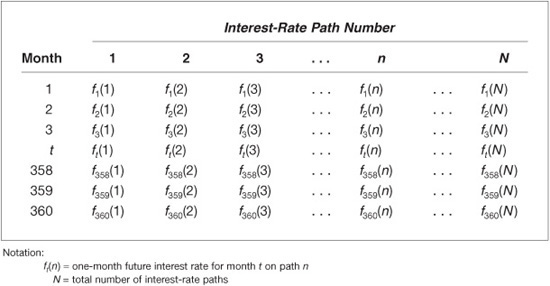
EXHIBIT 41–2
Simulated Paths of Mortgage Refinancing Rates

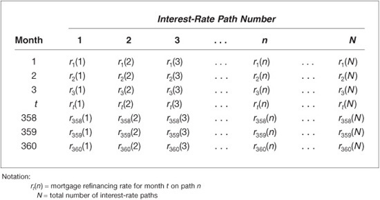
EXHIBIT 41–3
Simulated Cash-Flow on Each of the Interest-Rate Paths

Calculating the Present Value for a Scenario Interest-Rate Path

Given the cash-flow on an interest-rate path, its present value can be calculated. The discount rate for determining the present value is the simulated spot rate for each month on the interest-rate path plus an appropriate spread. The spot rate on a path can be determined from the simulated future monthly rates. The relationship that holds between the simulated spot rate for month T on path n and the simulated future one-month rates is

z_T(n) = {[1 + f₁(n)][1 + f₂(n)]⋅ ⋅ ⋅ [1 + f_T(n)]}^1/T − 1

where

z_T (n) = simulated spot rate for month T on path n

f_j (n) = simulated future one-month rate for month j on path n

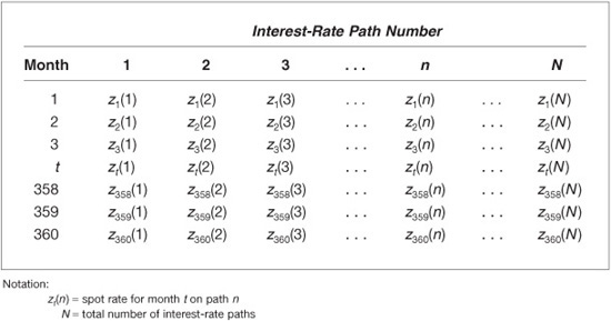
Consequently, the interest-rate path for the simulated future one-month rates can be converted to the interest-rate path for the simulated monthly spot rates, as shown in Exhibit 41–4. Therefore, the present value of the cash-flow for month T on interest-rate path n discounted at the simulated spot rate for month T plus some spread is

EXHIBIT 41–4
Simulated Paths of Monthly Spot Rates

where

PV[C_T (n)] = present value of cash-flow for month T on path n

         C_T(n) = cash-flow for month T on path n

         z_T(n) = spot rate for month T on path n

               K = spread

The present value for path n is the sum of the present value of the cash-flow for each month on path n. That is,

PV[path(n)] = PV[C₁(n)] + PV[C₂(n)] ⋅ ⋅ ⋅+ PV[C₃₆₀(n)]

where PV[path(n)] is the present value of interest-rate path n.

The option-adjusted spread is the spread K that when added to all the spot rates on all interest-rate paths will make the average present value of the paths equal to the observed market price (plus accrued interest). Mathematically, OAS is the spread K that will satisfy the following condition:

where N is the number of interest-rate paths.

This procedure for valuing a pass-through is also followed for a CMO tranche. The cash-flow for each month on each interest-rate path is found according to the principal repayment and interest distribution rules of the deal. In order to do this, a CMO structuring model is needed.

Selecting the Number of Interest-Rate Paths

Let’s now address the question of the number of scenario paths or repetitions N needed to value a CMO tranche. A typical OAS run will be done for 512 to 1,024 interest-rate paths. The scenarios generated using the simulation method look very realistic and furthermore reproduce today’s swap curve. By employing this technique, the money manager is effectively saying that swaps are fairly priced today and that the objective is to determine whether a specific tranche is rich or cheap relative to swaps.

The number of interest-rate paths determines how “good” the estimate is, not relative to the truth but relative to the OAS model used. The more paths, the more average spread tends to settle down. It is a statistical sampling problem.

Most OAS models employ some form of variance reduction to cut down on the number of sample paths necessary to get a good statistical sample.² Variance reduction techniques allow us to obtain price estimates within a tick. By this we mean that if the OAS model is used to generate more scenarios, price estimates from the model will not change by more than a tick. Thus, for example, if 1,024 paths are used to obtain the estimated price for a tranche, there is little more information to be had from the OAS model by generating more than that number of paths. (For some very sensitive CMO tranches, more paths may be needed to estimate prices within one tick.)

Interpretation of the OAS

The procedure for determining the OAS is straightforward, although time-consuming. The next question, then, is how to interpret the OAS. Basically, the OAS is used to reconcile value with market price. On the left-hand side of the last equation is the market’s statement: The price of a mortgage-backed security or mortgage derivative. The average present value over all the paths on the right-hand side of the equation is the model’s output, which we refer to as value.

What a money manager seeks to do is to buy securities whose value is greater than their price. A valuation model such as the one described earlier allows a money manager to estimate the value of a security, which at this point would be sufficient to determine whether to buy a security. That is, the money manager can say that this bond is 1 point cheap or 2 points cheap, and so on. The model does not stop here, however. Instead, it converts the divergence between price and value into a yield spread measure because most market participants find it more convenient to think about yield spread than about price differences.

The OAS was developed as a measure of the yield spread that can be used to reconcile dollar differences between value and price. But what is it a “spread” over? In describing the preceding model, we can see that the OAS is measuring the average spread over the swap spot-rate curve, not the swap yield-curve. It is an average spread because the OAS is found by averaging over the interest-rate paths for the possible spot-rate curves.

Option Cost

The implied cost of the option embedded in any mortgage-backed security can be obtained by calculating the difference between the OAS at the assumed volatility of interest rates and the static spread. That is,

Option cost = static spread – option-adjusted spread

The reason that the option cost is measured in this way is as follows: In an environment of no interest-rate changes, the investor would earn the static spread. When future interest rates are uncertain, the spread is less, however, because of the homeowner’s option to prepay; the OAS reflects the spread after adjusting for this option. Therefore, the option cost is the difference between the spread that would be earned in a static interest-rate environment (the static spread) and the spread after adjusting for the homeowner’s option.

In general, a tranche’s option cost is more stable than its OAS in the face of market movements. This interesting feature is useful in reducing the computational expensive costs of calculating the OAS as the market moves. For small market moves, the OAS of a tranche may be approximated by recalculating the static spread (which is relatively cheap and easy to calculate) and subtracting its option cost.

Other Products of the OAS Models

Other products of the valuation model are option-adjusted duration, option-adjusted convexity, and simulated average life.

Option-Adjusted Duration

In general, duration measures the price sensitivity of a bond to a small change in interest rates. Duration can be interpreted as the approximate percentage change in price for a 100 basis point parallel shift in the yield-curve. For example, if a bond’s duration is 4, this means a 100 basis point increase in interest rates will result in a price decrease of approximately 4%. A 50 basis point increase in yields will decrease the price by approximately 2%. The smaller the change in basis points, the better the approximated change in price will be.

The duration for any security can be approximated as follows:

where

P₋ = price if yield is decreased (per $100 of par value) by Δy

P₊ = price if yield is increased (per $100 of par value) by Δy

P₀ = initial price (per $100 of par value)

Δy = number of basis points change used to calculate P₋ and P₊

The standard measure of duration is modified duration. The limitation of modified duration is that it assumes that if interest rates change, the cash-flow does not change. While modified duration is fine for option-free securities such as Treasury bonds, it is inappropriate for mortgage-backed securities because projected cash-flows change as interest rates and prepayments change. When prices in the duration formula are calculated assuming that the cash-flow changes when interest rates change, the resulting duration is called effective duration.

Effective duration can be computed using an OAS model as follows: First, the bond’s OAS is found using the current term structure of interest rates. Next, the bond is repriced holding OAS constant but shifting the term structure. Two shifts are used; in one, yields are increased, and in the second, they are decreased. This produces the two prices, P₋ and P₊, used in the preceding formula. Effective duration calculated in this way is often referred to as option-adjusted duration, or OAS duration.

The assumption in using modified or effective duration to project the percentage price change is that all interest rates change by the same number of basis points; that is, there is a parallel shift in the yield-curve. If the term structure does not change by a parallel shift, then effective duration will not correctly predict the change in a bond’s price.

Option-Adjusted Convexity

The convexity measure of a security is the approximate change in price that is not explained by duration. Positive convexity means that if yields change by a given number of basis points, the percentage increase in price will be greater than the percentage decrease in price. Negative convexity means that if yield changes by a given number of basis points, the percentage increase in price will be less than the percentage decrease in price. That is, for a 100 basis point change in yield:

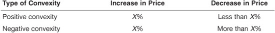
Obviously, positive convexity is a desirable property of a bond. A pass-through security can exhibit either positive or negative convexity depending on the prevailing mortgage rate relative to the rate on the underlying mortgage loans. When the prevailing mortgage rate is much higher than the mortgage rate on the underlying mortgage loans, the pass-through usually exhibits positive convexity. It usually exhibits negative convexity when the underlying coupon rate is near or above prevailing mortgage refinancing rates.

The convexity of any bond can be approximated using the formula

When the prices used in this formula assume that the cash-flows do not change when yields change, the resulting convexity is a good approximation of the standard convexity for an option-free bond. When the prices used in the formula are derived by changing the cash-flows (by changing prepayment rates) when yields change, the resulting convexity is called effective convexity. Once again, when an OAS model is used to obtain the prices, the resulting value is referred to as the option-adjusted convexity, or OAS convexity.

Simulated Average Life

The average life reported in an OAS model is the average of the average lives along the interest-rate paths. That is, for each interest-rate path, there is an average life. The average of these average lives is the average life reported in an OAS model.

Additional information is conveyed by the distribution of the average life. The greater the range and standard deviation of the average life, the more uncertainty there is about the tranche’s average life.

ILLUSTRATIONS

We use two deals to show how CMOs can be analyzed using the OAS methodology: a plain-vanilla sequential-pay structure and a PAC/support structure.

Plain-Vanilla Sequential-Pay Structure

As the name suggests, CMO tranches in a sequential-pay structure are amortized in sequence. The sequential-pay structure partitions the underlying mortgage collateral into bonds of varying maturities and durations, but does not allow the optionality of the bonds to be tailored.

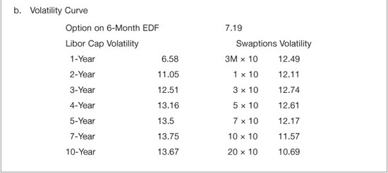
The plain-vanilla sequential-pay CMO bond structure in our illustration is FHLMC 3145, Collateral Group 5 analyzed as of June 7, 2007. The focus of our analysis is tranches AB, AC, and AJ. Exhibit 41–5 shows the swap yield spread and volatility curve at the evaluation date.

EXHIBIT 41–5
Par Curve and Volatility Curve as of 6/7/2007

Panel A of Exhibit 41–6 shows the OAS and the option cost for the collateral and the three tranches in the CMO structure. The OAS for the collateral is 24 basis points. Since the option cost is 32 basis points, the static spread is 56 basis points (24 basis points plus 32 basis points). As can be seen from Panel A of Exhibit 41–5, at the time this analysis was performed, the swap curve was not steep. As we noted earlier, in such a yield-curve environment, the static spread will not differ significantly from the traditionally computed yield spread. Thus, for the three tranches shown in Exhibit 41–6, the static spread is 27 for AB, 36 for B, and 52 for C. Notice that the tranches did not share the OAS equally. The same is true for the option cost. The value tended to go toward the longer bonds, something that occurs in the typical deal. Both the static spread and the option cost increase as the maturity increases. Notice that by purchasing tranches with the higher OAS, the manager is accepting greater interest rate risk as measured by the tranche’s effective duration.

Now let’s look at modeling risk. Examination of the sensitivity of the tranches to changes in prepayments and interest rate volatility will help us to understand the interaction of the tranches in the structure and who is bearing the risk.

We begin with prepayments. Specifically, we keep the same interest-rate paths as those used to get the OAS in the base case (the top panel of Exhibit 41–6), but reduce the prepayment rate on each interest-rate path to 80% of the projected rate.

As can be seen in Panel B of Exhibit 41–6, slowing down prepayments decreases the OAS and price for the collateral. This is so because the collateral is trading below par value. Tranches created by this collateral typically will behave the same way. However, if a tranche was created with a higher coupon, allowing it to trade below above, then it may behave in the opposite fashion. The exhibit reports two results of the sensitivity analysis. First, it indicates the change in the OAS. Second, it indicates the change in the price, holding the OAS constant at the base case.

EXHIBIT 41–6
OAS Analysis of FHLMC 3145 Classes AB, AC, and AJ (as of 6/7/2007)

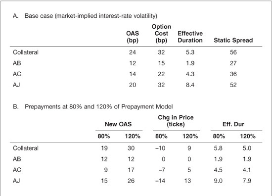
To see how a money manager can use the information in Panel B, consider tranche AC. At 80% of the prepayment speed, the OAS for this tranche decreases from 14 basis points to 9 basis points. If the OAS is held constant, the panel indicates that the buyer of tranche AC would lose $0.07 per $100 par value.

Notice that for the tranches AC and AJ reported in Exhibit 41–6, there is a loss from a slowdown in prepayments. This is so because all the sequential tranches in this deal were priced below par. Tranche AB’s OAS and price are not impacted by a slowdown in prepayments.

Also shown in Panel B of the exhibit is the second part of our experiments to test the sensitivity of prepayments: The prepayment rate is assumed to be 120% of the base case. The collateral’s price increases in this scenario because it is trading below par. This is reflected in the OAS of the collateral, which increases from 24 to 30 basis points.

Now look at the three tranches. Tranche AB’s price and OAS did not change. Hence, this tranche is prepayment insensitive from 80% to 120% of the base case. The OAS and price of the other two tranches increased.

Now let’s look at the sensitivity to the interest-rate volatility assumption. Two experiments are performed: reducing the volatility assumption to 4% of the base case and increasing it to 4% of the base case. These results are reported in Panel C of Exhibit 41–6. Reducing the volatility increases the dollar price of the collateral by $0.17 and increases the OAS from 24 to 41 basis points in the base case. This $0.17 increase in the price of the collateral is not equally distributed, however, among the three tranches. None of the increase went to tranche AC. Most of the increase in value is realized by the longest tranche, tranche AJ.

The OAS gain for each of the tranches follows more or less the effective durations of those tranches. This makes sense because the longer the duration, the greater the interest rate risk, and when volatility declines, the reward is greater for the accepted risk.

At the higher level of assumed interest-rate volatility, the collateral is adversely affected with the collateral’s loss distributed among the tranches in the expected manner: the longer the effective duration, the greater the loss.

Using the OAS methodology, a fair conclusion that can be made about this simple plain-vanilla structure is: What you see is what you get. A money manager willing to extend duration gets paid for that risk in this plain-vanilla structure.

PAC/Support Bond Structure

PAC structures are designed to create a stable set of bonds by directing the prepayment risk of the underlying collateral to other bonds (the supports) in the structure. One set of bonds (the PACs) is assigned a principal redemption schedule, which is given priority over principal payments to the remaining bonds (the supports) in the structure.

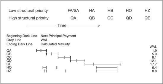
Now let’s look at how to apply the OAS methodology to a more complicated CMO structure, FHLMC 3104, Collateral Group 1. This $250 million agency CMO deal was issued on January 30, 2006 and analyzed on June 7, 2007 (so the interest-rate environment was that shown in Exhibit 41–5). A summary of the deal is provided in Exhibit 41–7. A diagram of the principal allocation is given in Exhibit 41–8. Shown in parentheses after each tranche’s name in Exhibit 41–7 is the type of tranche. There are five planned amortization class (PAC) tranches that are sequential-pay PACs and they have the high structural priority, as shown in Exhibit 41–8, while the other tranches are support bonds that have the low structural priority. Our focus will be on the five PAC tranches and the support tranches HO and HZ. We do not look at the floater and inverse floater support tranches (FA and SA, respectively).

EXHIBIT 41–7
Summary of FHLMC 3104, Collateral Group 1

EXHIBIT 41–8
Diagram of Principal Allocation Structure of FHLMC 3104 Collateral Group 1 (as of 6/7/2007)

Panel A of Exhibit 41–9 shows the base case OAS and the option cost for the collateral and all the tranches. The collateral OAS is 12 basis points, and the option cost is 28 basis points. The static spread of the collateral is 40 basis points. The 12 basis points of OAS did not get equally distributed among the tranches, as was the case with the plain-vanilla structure. Notice the high OAS for tranche HO the support principal-only tranche: 513 basis points. This tranche’s option cost is –83 basis points, suggesting that this tranche, according to the model, is cheap. For the sequential-pay PAC tranches we see that the longer the effective duration, the higher the OAS.

EXHIBIT 41–9
OAS Analysis of FHLMC 3104 Collateral Group 1 (as of 6/7/2007)

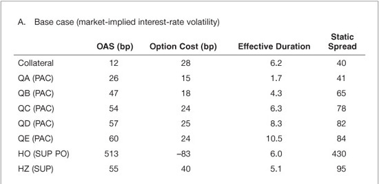
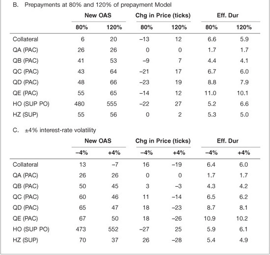
The next two panels in Exhibit 41–9 show the sensitivity of the OAS and the price (holding OAS constant at the base case) to changes in the prepayment speed (80% and 120% of the base case) and to changes in volatility (±4% of the base case). With respect to sensitivity to prepayments, the short-term PAC tranche QA and support bond HZ are insensitive for the prepayment range tested. For all of the other tranches, the OAS and price decrease with a decrease in prepayments. The opposite holds for an increase in prepayments.

The sensitivity of the collateral and the tranches to changes in volatility are shown in Panel C of Exhibit 41–9. The shorter-term PAC tranche (QA) is insensitive to changes in volatility. However, unlike with prepayments, support tranche HZ is sensitive to interest-rate volatility. For all of the tranches except tranche HO, OAS and price increase with a decline in volatility and decrease with an increase in volatility.

KEY POINTS

• Mortgage-backed securities are complex instruments. Traditional measures of valuation such as cash-flow yield and relative valuations such as yield spread or static spread are inadequate because of the prepayment option given to homeowners.

• The OAS valuation model is a sophisticated analytical tool available to assess value.

• The results of an OAS model should be stress-tested for modeling risk: alternative prepayment and interest rate volatility assumptions.

• OAS analysis helps the investors understand where the risks are in a CMO deal and to identify tranches that based on the model are fairly priced and those are possibly cheap or rich.

• Compared with a sophisticated analytical tool such as OAS analysis, traditional static analysis can lead to very different conclusions about the relative value of the tranches in a deal.