CHAPTER
FORTY-SIX
INTRODUCTION TO MULTIFACTOR RISK MODELS IN FIXED INCOME AND THEIR APPLICATIONS

ANTHONY LAZANAS, PH.D.

Managing Director
Barclays Capital

ANTÓNIO BALDAQUE DA SILVA, PH.D.

Director
Barclays Capital

RADU GBUDEAN, PH.D.

Vice President
Barclays Capital

ARNE D. STAAL, PH.D.

Director
Barclays Capital

Risk management is an integral part of the investment process. Risk models are central to this practice, allowing managers to quantify and analyze the risk embedded in their portfolios. Risk models provide managers with insight into the different sources of risk in a portfolio, helping them to control their exposures and understand the contributions of different portfolio components to total risk. They help portfolio managers in their decision-making process by providing answers to important questions such as: How does my long-duration exposure affect portfolio risk? Does my underweight in diversified financials hedge my overweight in banks? Risk models are also widely used in various other areas such as in portfolio construction, performance attribution, and scenario analysis.

In this chapter we introduce linear multifactor risk models and illustrate how they can be helpful for the analysis of the risk of fixed income portfolios. We review the major sources of risk in fixed income securities and introduce a set of appropriate risk factors. We also present several applications of risk models for effective portfolio construction and management. In Chapter 47 we will go through a detailed risk model report of a specific portfolio and highlight the information and insights it can provide to a portfolio manager.

The authors would like to thank Bruce Phelps and Andy Sparks for their valuable comments.

MOTIVATION AND STRUCTURE UNDERLYING FIXED INCOME MULTIFACTOR RISK MODELS

In this section, we discuss the motivation and structure behind fixed income multifactor risk models.

Let us assume that a portfolio manager wants to estimate and analyze the volatility of a large portfolio of fixed income instruments. A straightforward idea would be to compute the volatility of the historical returns of the portfolio and use this measure to forecast future volatility. However, this framework does not provide any insight into the relationships between different securities in the portfolio or the major sources of risk. For instance, it does not assist a portfolio manager interested in diversifying a portfolio or constructing a portfolio that has better risk-adjusted performance. Additionally, the characteristics of a fixed income portfolio change substantially over time, for instance, as instruments mature or are subject to credit events.

Instead of estimating the portfolio volatility using historical portfolio returns, a portfolio manager could utilize a different strategy. The portfolio return is a function of individual instrument returns (e.g., Treasury securities, corporate bonds, credit derivatives, municipal bonds, interest rate swaps, and so on) and the market weights of these securities in the portfolio. Using this, the forecasted volatility of the portfolio can be computed as a function of the weights (w) and the covariance matrix (Σ_S) of the instrument returns in the portfolio:

where the superscript T denotes a matrix transpose. This covariance matrix can be decomposed into individual instrument volatilities and the correlations between returns.

Volatilities measure the riskiness of individual instrument returns, and correlations represent the relationships between the returns of different instruments. By measuring these correlations and volatilities, the portfolio manager can gain insight into her portfolio related to the riskiness of different parts of the portfolio or how the portfolio can be diversified. As outlined above, to estimate the portfolio volatility we need to estimate the correlation between each pair of instruments. Unfortunately, this means that the number of parameters to be estimated grows quadratically with the number of instruments in the portfolio.¹ For most practical portfolios, the relatively large number of constituents makes it difficult to estimate the relationship between instrument returns in a robust way. Moreover, this framework uses the history of individual instrument returns to forecast future security return volatility. However, instrument characteristics are dynamic and hence using returns from different time periods may not produce good forecasts.² These drawbacks constitute the motivation for multifactor risk models discussed in this chapter.

One of the major characteristics of multifactor models is their ability to describe the return of a portfolio using a relatively small set of variables, called factors. These factors should be designed to capture broad (systematic) market fluctuations, but should also be able to capture specific nuances of individual portfolios. For instance, a broad fixed income market factor would capture the general movement in the fixed income markets, but not the varying behavior across types of instruments. If, for example, a portfolio is heavily biased toward the long end of the U.S. Treasury yield-curve, or is tilted toward credit bonds of particular industries, the broad market factor may not allow for a good representation of the portfolio’s return. Other factors might be needed to capture these more specific sources of risk.

Most factor models are linear, in the sense that the total return is decomposed into the sum of the contributions of the factors (referred to as the systematic return) and an idiosyncratic component. Systematic return is the component of total return due to movements in the common (market-wide) risk factors. On the other hand, idiosyncratic return can be described as the residual component that cannot be explained by the systematic factors. Under most factor models, idiosyncratic returns are uncorrelated across issuers. Therefore, correlations across securities of different issuers are driven by their exposures to the systematic risk factors, and the correlation between those factors.

The following equation demonstrates the systematic and the idiosyncratic components of total return for security s:

r_s = L_s × F + ε_s

The systematic return is the product of the instrument’s loadings (L, also called sensitivities) to the systematic risk factors and the returns of these factors (F). The idiosyncratic return is given by ε_s.

Under these models, the portfolio volatility can be estimated as

Here L_p are the loadings of the portfolio to the risk factors (determined as the weighted average of individual instrument loadings) and Σ_F is the covariance matrix of factor returns. Ω is the covariance matrix of the idiosyncratic security returns. Typically, the idiosyncratic return of securities is assumed uncorrelated. Therefore, this covariance matrix is diagonal, with all elements outside its diagonal being zero.³ As a result, the idiosyncratic risk of the portfolio is diversified away as the number of securities in the portfolio increases. This is, of course, the diversification benefit attained when combining uncorrelated exposures.

For most practical portfolios, the number of factors is significantly smaller than the number of instruments in the portfolio. Therefore, the number of parameters in Σ_F is much smaller than in Σ_S, leading to a generally more robust estimation. Moreover, the factors can be designed in a way that they are relatively more stable than individual stock returns, leading to models with potentially better predictability. In this setting, the changing nature of each particular instrument can be captured through its loadings to the different risk factors.

Another very important advantage of using factor models is the detailed insight they can provide into the structure and properties of portfolios. These models characterize instrument returns in terms of systematic factors that (can) have intuitive economic interpretations. Linear factor models can provide important insights regarding the major systematic and idiosyncratic sources of risk and return. This analysis can help managers to better understand their portfolios and can guide them through the different tasks they perform, such as rebalancing, hedging, or tilting of their portfolios.

Naturally, the success of a risk model depends on its ability to interpret historical and current data in order to formulate estimates of future portfolio risk. It should therefore seek to discover properties of the data that are quasi-predictable; that is, that the error in the estimate of future realizations—given all information known today—is relatively small. For example, it is notoriously difficult to predict the expected return of a financial asset. On the other hand, historical data contain sufficient information to allow risk models to provide good estimates of the volatility of future returns. Nevertheless, one should never forget that even the most sophisticated risk model can only provide an estimate of risk. It is well known that financial markets are subject to event risk (i.e., a sudden change in market conditions cause by geopolitical or financial events). Such events are usually followed by a period of large negative returns of risky assets, large positive returns of assets considered as safe havens, significantly higher volatility, and very high (positive or negative) correlations. It is impossible for a risk model to predict when such events will occur. Therefore, it is useful to complement model-based risk management and portfolio construction with what-if analysis, which estimates portfolio return and risk under stressed conditions; that is, scenarios with extreme realizations of market returns and a covariance matrix with much higher volatilities and absolute correlations.

FIXED INCOME RISK MODELS

Fixed income securities are exposed to many different types of risk. Multifactor risk models in this area capture these risks by first identifying common sources along different dimensions, the systematic fixed income risk factors. All risk not captured by these systematic factors is considered idiosyncratic, and is determined by the choice of systematic risk factors. Typically, fixed income systematic risk factors are divided into two sets: those that influence securities across asset classes (e.g., yield-curve risk) and those specific to a particular asset class (e.g., prepayment risk in securitized products).

There are many ways to define systematic risk factors. For instance, they can be defined purely by statistical methods, observed in the markets (e.g., a yield-curve), or estimated from asset returns. In fixed income, the standard approach is to use pricing models to calculate the analytics that are the natural candidates for risk factor loadings (L, in the notation presented earlier). In this setting, the risk factors are either observable (e.g., the movements in the yield-curve) or estimated from regressing cross-sectional asset returns on instrument sensitivities. This is the approach taken in the Barclays Capital Global Risk Model,⁴ which is the model used for illustration throughout this chapter.

In this risk model, the forecasted risk of the portfolio is driven by both a systematic and an idiosyncratic (also called specific, nonsystematic, or concentration) component. The forecasted systematic risk is a function of the mismatch between the portfolio and the benchmark in the exposures to the risk factors, such as yield-curve or spreads. The (net) portfolio exposures are aggregated from security-level analytics. The systematic risk is also a function of the volatility of the risk factors, as well as the correlations between the risk factors. In this setting, the correlation of returns across securities is driven by the correlation of systematic risk factors these securities load on. Because the model uses security-level returns and analytics to estimate the factors, it can recover the idiosyncratic return for each security. This is the return net of all systematic factors. The use of detailed level analysis of idiosyncratic returns allows for the estimation of rich specifications of idiosyncratic risk.

Systematic Risk Factors

The precise definition of systematic risk factors depends on the purpose of the factor model, but in general we can highlight several categories of risk factors that drive fixed income risk.

Curve Risk

Curve risk is the major source of risk across fixed income instruments. This kind of risk is embedded in virtually all fixed income securities; therefore, mismatches in curve profiles relative to a benchmark are often the main drivers of portfolio risk.

When analyzing curve risk, we should use the curve of reference in which we are interested. Depending on the portfolio and circumstances, this is typically the government or swap curve.⁵ In calm periods, the behavior of the swap curve tends to match that of the government curve. However, during liquidity crises (e.g., the Russian crisis in 1998 or the credit crisis in 2008), they can diverge significantly. To capture these different behaviors adequately, one may use the following decomposition: for government products, the curve risk is assessed using the government curve. For all other products in the portfolio (that usually trade off the swap curve), this risk is measured using both the Treasury curve and swap spreads (i.e., the spreads between the swap and the government curve). Other curve decompositions are also possible.

The risk associated with each of these curves can be described by the exposure the portfolio has to different points along the curve combined with the volatility and correlation of the movement of such curve points. Sometimes a convexity term is required to capture the second-order exposure to curve changes of instruments with long tenors or embedded optionality, such as mortgage-backed securities. For a typical portfolio, a good description of the curve can be achieved by looking at a relatively small number of points along the curve (called key-rates), for example 6-month, 2-year, 5-year, 10-year, 20-year, and 30-year. An alternative set of factors used to capture yield-curve risk can be defined using statistical analysis of the historical realizations of the various yield-curve points. The statistical method used most often is principal component analysis (PCA). This method defines factors that are statistically independent of each other. Typically three or four such factors are sufficient to explain the risk associated with changes of yields across the yield-curve. PCA analysis has several shortcomings and must be used with caution. Using a larger set of economic factors like the key-rate points described above is more intuitive and captures the risk of specialized portfolios better. For these reasons, many portfolio managers favor the key-rates approach in most risk analysis problems.

Credit Risk

Instruments issued by corporations or entities that may default are said to have credit risk. The holders of these securities demand additional yield—in excess of the risk-free yield—to compensate for that risk. This extra yield is usually measured as a spread to a reference curve. For instance, for corporate bonds the reference curve is usually the swap curve. The level of credit-spreads determines to a large extent the credit risk exposure associated with the portfolio.⁶

There are several characteristics of credit bonds that are naturally associated with systematic sources of credit-spread risk. For instance, depending on the business cycle, particular industries may be going through especially tough times. So industry membership is a natural systematic source of risk. Similarly, bonds with different credit ratings are usually treated as having different levels of credit risk. Credit rating could be another dimension one can use to measure systematic exposure to credit risk. Finally, the country of the issuer is another source of systematic risk for credit bonds. Given these observations, it is common to see factor models for credit risk using country, industry, and rating as the major systematic risk factors. Recent research suggests that risk models that directly use the spreads of the bonds instead of their ratings perform better for risk analysis over relatively short/medium horizons.⁷ Under this approach, the loading of a particular bond to a credit-risk factor would be the commonly used spread duration, but now multiplied by the bond’s spread. The loading is termed Duration Times Spread (denoted DTS) and is described in Chapter 55. By directly using the spread of the bond in the definition of the loading to the credit risk factors, we do not need to assign specific risk factors to capture the rating or any similar quality-like effect. It will be automatically captured by the spread level incorporated into the bond’s loading to the credit risk factor, and will adjust as the spread of the bond changes. In this setting, we still could use different systematic risk factors, for example, to distinguish among credit risk coming from different industries.⁸

Prepayment Risk

Securitized products are generally exposed to prepayment risk. The most common of the securitized products are the residential mortgage-backed securities (RMBS or simply MBS). These securities represent pools of deals that allow the borrower to prepay their debt before the maturity of the loan/deal, most typically when prevailing lending rates are lower. This option means an extra risk to the holder of the security, the risk of holding cash exactly when reinvestment rates are low. Therefore, these securities have two major sources of risk: interest rate (including convexity) and prepayment risk.

Some part of the prepayment risk can be expressed as a function of interest rates via a prepayment model. This risk will be captured as part of interest-rate risk using the key-rate durations and the convexity. Convexity, which is usually negative for these instruments, is a significant source of risk. Negative convexity has a detrimental effect on the market value of an instrument—compared with one with positive or zero convexity—when interest rates move significantly in either direction. Indeed, decreasing interest rates cause prepayments to increase thereby reducing the price appreciation because of the falling rates. Conversely, rising interest rates intensify the price depreciation the instrument suffers with higher rates.

The remaining part of prepayment risk—that is not captured by the prepayment model—must be modeled with additional systematic risk factors. Typically, the volatility of prepayment speeds (and therefore of risk) on MBS depends on three characteristics: program/term of the deal, if the bond is priced at discount or premium (e.g., if the coupon on the bond is bigger than the current mortgage rates), and how seasoned the bond is. This analysis suggests that the systematic risk factors in a risk model should span these three characteristics of the securities.

Implied Volatility Risk

Many fixed income securities have embedded options (e.g., callable bonds). This means that the expected future volatility (implied volatility⁹) of the interest rate or other discount curves used to price the security plays a role in the value of that option. If expected volatility increases, options generally become more expensive, thereby affecting the prices of bonds with embedded options. For example, callable bonds will become cheaper with increasing implied volatility since the bondholder is short optionality (the right of the issuer to call the bond). Therefore, the exposure of the portfolio to the implied volatility of the yield-curve is also a source of risk that should be accounted for. The sensitivity of securities to changes of implied volatilities is typically measured by vega, which is calculated using the security pricing model. Implied volatility factors can be either calculated from the market prices of liquid fixed income options (caps, floors, and swaptions), or implied by the returns of bonds with embedded options within each asset class.

Liquidity Risk

Many fixed income securities are traded over-the-counter, in decentralized markets. Some trade infrequently, making them illiquid. It is therefore hard to establish their fair price. These bonds are said to be exposed to liquidity risk. The holder of illiquid bonds would have to pay a higher price to liquidate a position, usually meaning selling at a discount. This discount is uncertain and varies across the business cycle. For instance, the discount can be significant in a liquidity crisis, such as the one of 2008. The uncertainty about this discount means that, everything equal, a more illiquid bond will be riskier. This extra risk can be captured through liquidity risk factors. For instance, in the Treasury markets, one generally refers to the difference in volatility between an on-the-run and an off-the-run Treasury bond as liquidity risk.

Inflation Risk

Inflation-linked securities are priced based on the expectation of future inflation. Uncertainty about this variable adds to the volatility of the bond over and above the volatility from other sources of risk, such as nominal interest rates. Expected inflation is not an observed variable in the marketplace but can be extracted from the prices of inflation-linked government bonds and inflation swaps. Expected inflation risk factors can be constructed by summarizing this information. The sensitivity of securities to expected inflation is calculated using a specialized pricing model and is usually called inflation duration.

Tax-Policy Risk

Many municipal securities are currently tax-exempt. This results in added benefit to their holders. This benefit—incorporated in the price of the security—depends on the level of exemption allowed. Uncertainty around tax policy—tax-policy risk—adds to the risk of these securities. Once again, tax-policy risk factors cannot be observed in the marketplace and must be extracted from the prices of municipal securities. The return of municipal securities in excess of interest rates is driven partially by tax-policy expectations changes. However, it is also driven by changes in the creditworthiness of the municipal issuers as well as other factors. In this case, it is difficult to separate tax-policy risk factors from other factors driving municipal bond spreads. Therefore, instead of specific tax-policy factors, we usually extract factors representing the overall spread risk of municipal securities. This exercise is performed in a similar way to the credit risk model, in which securities are partitioned into groups of “similar” risk by geography, bond type (general obligation vs. revenue), tax status, and the like.¹⁰

There are other sources of systematic risk we did not detail in this section. They may be important sources of risk for particular portfolios. Specific risk models and factors can be designed to address them.

Idiosyncratic Risk

Once all systematic factors and loadings are determined, the residual idiosyncratic return of a security can be computed as the component of its total return that cannot be explained by the systematic factors. Idiosyncratic return can be a significant component of total return for individual instruments, but tends to decrease rapidly for portfolios of instruments as the number of instruments increases and concentration decreases (the aforementioned diversification effect).

The major inputs to the computation of idiosyncratic risk are instrument characteristics and historical idiosyncratic returns of the instruments. The use of idiosyncratic residual returns allows the risk modeler to find empirical relationships between characteristics such as instrument spread, spread duration, industry membership, and idiosyncratic volatility. This mapping of instrument characteristics to idiosyncratic volatility allows for the modeling of new issues and issues with characteristics that change over time. As mentioned before, idiosyncratic returns of different issuers are assumed to be uncorrelated. However different securities from the same issuer, or securitized products with related underlying instruments, can show a certain level of co-movement, as they are all exposed to specific events affecting their common issuer that are not captured by systematic risk factors. Interestingly, this co-movement is not perfect or static. Certain news can potentially affect the different securities issued by the same company (e.g., equity, credit default swaps, bonds, or equity options) in different ways. Moreover, this relationship changes with the particular circumstances of the firm. For instance, returns from securities with claims to assets of the firm should be more highly correlated if the firm is in distress. A good multi-asset class risk model should be able to capture these phenomena regarding idiosyncratic risk.

APPLICATIONS OF RISK MODELING

In this section, we illustrate several standard risk model applications used for portfolio management. All applications make use of the fact that the risk model translates the characteristics a portfolio may have across many different dimensions, into a common, comparable set of numbers. In some of them—risk budgeting and portfolio rebalancing—an optimizer that uses the risk model as an input is the optimal setting to perform the exercise.

The investment process of a typical portfolio manager involves different stages. Given the investment universe and objective, the steps usually consist of portfolio construction, risk prediction, and performance evaluation. These steps are iterated throughout the investment cycle over each rebalancing period. The examples in this section highlight the portfolio construction and risk analysis steps that employ a factor model. Additionally, scenario analysis can be employed in both the portfolio construction and risk evaluation phases of the portfolio process. This exercise allows the manager to gain additional intuition regarding portfolio exposures and how the portfolio may behave under particular economic circumstances. It usually takes the form of stress testing potential portfolio losses under historical or hypothetical scenarios. It can also show the sensitivity of the portfolio to particular movements in economic and financial variables. The last application in this chapter illustrates this kind of analysis.

Portfolio Construction and Risk Budgeting

As discussed, fixed income portfolios are exposed to a diverse set of risk factors. During the portfolio construction exercise, the manager must carefully choose the exposure to such factors in order to achieve the highest possible portfolio return subject to risk and other constraints. Risk models help portfolio managers achieve this in an objective and quantifiable way and are increasingly used for portfolio construction, usually with the help of an optimization engine. In this section, we illustrate how a portfolio manager would use this engine to formulate client objectives and constraints in the context of risk model-based portfolio construction.¹¹

Portfolio managers can have a broad array of mandates. Some—typically referred to as indexers—are required to follow a given benchmark index with the minimum possible deviation. Their goal is to minimize the tracking error volatility of the portfolio versus the index while also keeping portfolio transaction costs as small as possible. Others, the enhanced indexers, are allowed some leeway to deviate from the benchmark in order to achieve superior returns. The leeway can be expressed as a set of rules constraining the exposure to risk factors, but it is often prescribed as a risk budget; that is, an upper limit in a statistical measure of deviation between the portfolio and its benchmark. The tracking error volatility (TEV) of the return of the portfolio net of the benchmark is the most common of such measures. Finally, the absolute return portfolio managers, do not have to track a benchmark but are instead aiming at the highest possible portfolio return, potentially subject to leverage, portfolio composition, exposure, and risk constraints. In all cases, the manager has to merge all views and constraints into a final portfolio. When constructing the portfolio, how can the competing views be managed, while respecting the risk budget? How can the views be combined to minimize the risk? What tradeoffs can be made? Risk models are widely used to perform this exercise in a systematic and objective manner: They can measure the risk of each view as well as the correlation between different views, and arrive at portfolios that optimally trade-off the risks and expected returns associated with each of the views.

We illustrate this by a simple example of a portfolio construction exercise using a risk model. Consider a fixed income portfolio manager who is benchmarked to the Barclays Capital U.S. Aggregate index. The manager’s mandate is to outperform the benchmark with a risk-budget of 20 bp/month (i.e., the portfolio’s TEV should remain within this bound on a monthly basis). Before formulating views and constraints, and deciding how to implement them, the manager needs to choose an investment universe. Since the benchmark is the Barclays Capital U.S. Aggregate Index, the manager could choose the investment universe to be all issues in this index with outstanding amount in excess of $300 million. The selection of this investment universe ensures that securities with small amounts of outstanding notional will not be selected in the portfolio, potentially increasing overall portfolio liquidity and decreasing transaction costs. With the risk budget in mind, the manager chooses to minimize total portfolio TEV relative to the benchmark. (The manager could potentially consider other risk-based objectives such as maximizing the Sharpe ratio.) This means the manager is giving leeway to the risk model to choose a portfolio from the tradable universe that minimizes the risk relative to the benchmark, in this case the Barclays Capital U.S. Aggregate Index. Finally, the manager formulates constraints and views.

Let us assume for the purpose of this illustration that the amount of funds to be invested is $100 million. With that in mind, and in order to avoid buying small amounts of securities, the manager decides to implement the portfolio using a maximum of 100 positions. Given views on the market environment, the manager wants the portfolio to be long duration against the benchmark, between 0.40 and 0.60 years, and have a spread advantage of 150 bp to 200 bp over the benchmark. Finally, to ensure a certain amount of diversification in portfolio positions, the manager imposes a maximum under/overweight of 3% per issuer relative to the benchmark.¹²

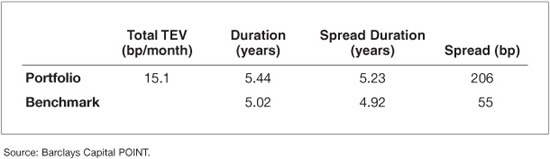
Our portfolio manager incorporates all these settings into an optimization problem, and finds a solution that reflects the optimal tradeoff between the constraints and risks through the optimization engine. The result is a recommended portfolio that satisfies the constraints while minimizing total risk. Specifically, the resulting portfolio—that we will follow throughout this section—consists of 100 securities, has a predicted TEV of 15.1 bp/month, interest-rate duration of 5.44 years, and option-adjusted spread of 206 bp (Exhibit 46–1). Using a factor-based risk model and an optimization engine, the resulting portfolio incorporates the manager’s views while staying within its risk budget and ensuring that all additional constraints are satisfied.

EXHIBIT 46–1
Portfolio and Benchmark Characteristics of Sample Portfolio

Analyzing Portfolio Risk

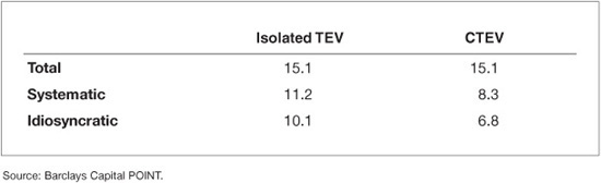
The main application of risk models is risk measurement of portfolios relative to their benchmark. Risk analysis based on multifactor models can take many forms: from a relatively high-level aggregate approach, to an in-depth analysis of the risk properties of individual instruments and groups of instruments. Multifactor fixed income risk models provide the tools to perform the analysis of portfolio risk in many different dimensions, including exposures to risk factors, security/factor contributions to total risk, and risk analysis at the issuer level. For instance, as previously described, this risk can be decomposed into a systematic and an idiosyncratic component. Exhibit 46–2 shows that the portfolio has total TEV of 15.1 bp/month, systematic TEV of 10.4 bp/month, and idiosyncratic TEV of 10.1 bp/month. Since systematic risk and idiosyncratic risk are independent, they constitute isolated (uncorrelated) risk sources of the portfolio and therefore we have

EXHIBIT 46–2
Portfolio Risk Results of Sample Portfolio in bp/Month

An alternative way to describe the manner in which different risk sources impact overall portfolio risk is through risk attribution. Risk attribution allows a manager to decompose portfolio volatility in an additive way into contributions to TEV. Exhibit 46–2 reports that the contribution to total TEV (CTEV) from systematic risk factors is 8.3 bp/month, whereas idiosyncratic risk contributes 6.8 bp/month.¹³

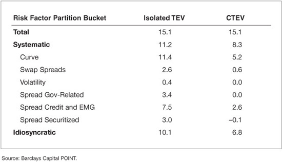
The risk attribution approach can be used to further decompose overall portfolio risk into contributions from different buckets. The buckets can represent groups of securities (e.g., industry buckets) or risk factors (e.g., factors related to curve or to credit-spreads). This flexible decomposition allows portfolio managers to gain a detailed understanding of how different securities and risk exposures affect overall portfolio risk.

Exhibit 46–3 shows the isolated TEV as well as the contributions to TEV for the sample portfolio. In this exhibit, we choose to partition risk across systematic risk factors (plus the idiosyncratic risk), but many other partitions are possible. In this example, the largest contribution within systematic risk comes from the exposure to “Curve” factors, with a CTEV of 5.2 bp/month. As we saw before, idiosyncratic exposure is also a large component of the risk in this portfolio, with a contribution of 6.8 bp/month to total risk. Notice the difference between isolated TEV and contribution to TEV for our factor partition—isolated TEV reflects the risk of the partition buckets in isolation—while contribution to TEV includes risk driven by correlations among the different buckets.

EXHIBIT 46–3
Portfolio Risk Contributions of Sample Portfolio in bp/Month

In addition to overall portfolio TEV and partition-based contributions to TEV, there are many additional risk analytics that can be computed on the basis of a linear factor risk model, such as betas with respect to the benchmark, liquidation effect to TEV, and marginal contributions to risk. Different users will use these analytics for different purposes and to different degrees.

Portfolio Rebalancing

Most managers rebalance their portfolios at regular intervals to reflect changing views and market circumstances. For instance, as time goes by, the characteristics of the portfolio may drift away from targeted levels. This may be due to the aging of its holdings, changes in the market environment, or issuer-specific events such as defaults. The periodic realignment of a portfolio to its investment guidelines and changing investment views is called portfolio rebalancing. Similar needs arise in many different contexts: when managers receive extra cash to invest, receive minor changes to their mandate, want to tilt positions toward their views, and the like. As with the initial portfolio construction, a risk model is very useful in the rebalancing exercise. During rebalancing, typically the portfolio manager seeks to sell bonds currently held and replace them with others having properties more consistent with the overall portfolio goals. Such buy and sell transactions are costly and their cost must be weighed against the benefit from moving the portfolio closer to its desired profile. A risk model can tell the manager how much risk reduction (or increase) a particular set of transactions can achieve in order to evaluate the risk adjustment benefits relative to the transaction cost.

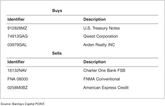
As an example, suppose the portfolio manager in our illustration wants to reduce the imbalances the portfolio has against the benchmark. Specifically, the manager wants to lower the net portfolio duration from 0.42 years to a value between 0.2 years and 0.4 years. After looking at the portfolio’s industry profile, the manager also decides to reduce the existing 6% overweight in the banking industry to about 4%. In addition, the manager lowers the minimum acceptable excess spread to 100 bp. To avoid high transaction costs, the manager also imposes the rebalancing to be done with no more than 30 trades. Finally, let us assume no portfolio inflows or outflows so the portfolio market value must remain unchanged. Starting from the original portfolio of 100 securities, a risk model and optimization engine can be employed to achieve optimal rebalancing by adjusting some of the constraints to reflect the portfolio manager’s new objectives.

Exhibit 46–4 shows the largest trades suggested by the optimizer, in terms of market value. Not surprisingly, the largest sell recommendations are of financial companies. To replace them, the optimizer—using the risk model—recommends a larger position of Treasury and corporate bonds. (Corporates are required in order to keep the spread of the portfolio at the desired level.)

EXHIBIT 46–4
Proposed Trading List

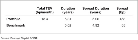
Interestingly, the rebalancing and extra constraints imposed on the optimization problem did not materially change the risk of the portfolio. Exhibit 46–5 shows that the total TEV of the portfolio actually decreased to 13.4 bp/month. This is largely due to an extra 13 positions added to the portfolio in the rebalancing (that now has 113 securities). These extra securities allowed the portfolio to reduce both its systematic and idiosyncratic risk.

EXHIBIT 46–5
Rebalanced Portfolio and Benchmark Characteristics

Scenario Analysis

Scenario analysis is a popular tool both for risk management and portfolio construction. In this section, we illustrate a way to construct scenarios based on factor models. In this context, a portfolio manager express views on the returns of particular financial variables, indices, securities or risk factors and the scenario analysis tool (using the risk model) calculates their impact on the portfolio’s (net) return.

Typically in this kind of scenario analysis, the views one has are only partial. This means one can have specific views on how particular macro variables, asset classes, or risk factors will behave, but it is unlikely to have views on all risk factors to which the portfolio under analysis is exposed. This is where risk models can be useful. At the heart of the linear factor models lies a set of risk factors and the covariance matrix between them. Under certain statistical assumptions, the covariance matrix can be used to “complete” specific partial views or scenarios and deliver a complete picture of the impact of the scenario in the return of the portfolio. Mechanically, what happens is the following. First, the manager translates the views into realizations of a subset of risk factors. Next the scenario is completed—using the risk model covariance matrix—to get the realizations of all risk factors. Finally, the portfolio’s (net) loadings to all risk factors are used to get its (net) return under that scenario (by multiplying the loadings by the factor realizations under the scenario). This construction implies a set of assumptions that should be carefully understood. To begin with, it is assumed that the manager can represent or translate views as risk factor returns. So a view about the unemployment rate, which is typically not used as a risk factor,¹⁴ cannot be used in this context. Also, to “complete” the scenario, we generally assume a stationary and normal multivariate distribution among all factors. Although these assumptions make this analysis less appropriate for looking at extreme events or regime shifts, for instance, the analysis can be very useful in many circumstances.

As an example, consider using factor-based scenario analysis to compute the model-implied empirical durations of the original portfolio of a 100 securities (i.e., before rebalancing) analyzed in detail previously in this chapter. In particular, suppose the portfolio manager has the view that interest rates will fall by 25 bp over the next month. Exhibit 46–6 shows that under this scenario, the portfolio returns 116 bp, against the 111 bp of the benchmark. As expected given the longer duration, the portfolio outperforms the benchmark. Due to the other exposures present in the portfolio and benchmark and their average negative correlation with the curve factors—for instance, a 25 bp fall in rates under this setting implies a 5% increase in corporate spread levels—the model duration implied by the scenario for the portfolio is 4.64 (= 116/25), while the analytical duration is 5.44. The scenario shows a similar decrease in the benchmark’s duration. The net model duration of the portfolio is only 0.22, almost half of its 0.42 net analytical duration.

EXHIBIT 46–6
Scenario Analysis: Analytical and Model-Implied Durations

Another characteristic imposed while constructing the portfolio was a targeted higher spread. The portfolio construction exercise resulted in an OAS for the portfolio of 206 bp against a spread level of 55 bp for the benchmark. The portfolio manager might be concerned with portfolio losses should spreads increase. To evaluate this risk, the portfolio manager can construct two scenarios. In the first scenario, credit-spreads widen by 20%, other spread risk factors move as implied by the credit-spread moves, but interest rates remain unchanged. In the second scenario, interest rates moves are implied by the credit-spread move. Exhibit 46–7 displays the results of the two scenarios. In the first scenario, the portfolio suffered significant losses of 0.84%. The benchmark which has a much lower spread suffers lower losses of 0.64% and the net result is –20 bp of net return. This number is very different from a back of the envelope calculation that uses portfolio-level analytics to estimate the return. The calculation is much more intricate and takes into account the security level portfolio composition, as well as the implied moves of other sources of risk such as swap and mortgage spreads.

EXHIBIT 46–7
Scenario Analysis: Corporate Spread Increase of 20%

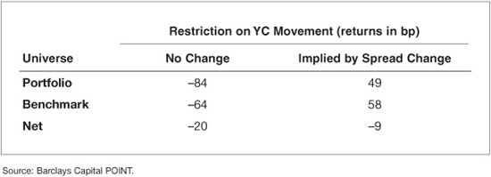
Things look better in the second scenario, where the net return of the portfolio versus the benchmark is only –9 bp. In fact, in this case both the portfolio and the benchmark exhibit positive returns of 0.49% and 0.58%, respectively, illustrating that this is a very different type of scenario. Indeed, the large spread widening implies a 25 bp fall in interest rates, which is sufficient to overcome the losses from the spread widening for both the portfolio and the benchmark. Since the portfolio has interest rate duration that is 0.42 years longer than the benchmark, it enjoys a relative improvement in net return of about –0.42 × –25 bp = +10.5 bp that partially offsets the losses from the widening of credit spreads.

These very simple examples illustrate how one can look at reasonable scenarios to study the behavior of the portfolio or the benchmark under different environments. This type of factor-based scenario analysis can significantly increase the intuition the portfolio manager has regarding the results from the risk model.

KEY POINTS

• Risk models describe the different imbalances of a portfolio using a common language. The imbalances are combined into a consistent and coherent analysis reported by the risk model.

• Risk models provide important insights regarding the different tradeoffs existing in the portfolio. They provide guidance regarding how to balance them.

• The fundamental systematic risk of all fixed income securities is interest rate and term structure risk. This is captured by factors representing risk-free rates and swap spreads of various maturities.

• Excess (of interest rates) systematic risk is captured by factors specific to each asset class. The most important components of such risk are credit risk and prepayment risk. Other risks that can be important are volatility, liquidity, inflation, and tax policy.

• Idiosyncratic risk is diversified away in large portfolios and indices, but can become a very significant component of the total risk in small portfolios. The correlation of idiosyncratic risk of securities of the same issuer must be modeled very carefully.

• A good risk model provides detailed information about the exposures of a complex portfolio and can be a valuable tool for portfolio construction and management. It can help managers construct portfolios tracking a particular benchmark, express views subject to a given risk budget, and rebalance a portfolio while avoiding excessive transaction cost. Further, by identifying the exposures in which the portfolio has the highest risk sensitivity, it can help a portfolio manager reduce (or increase) risk in the most effective way.