CHAPTER
FORTY-EIGHT
HEDGING INTEREST-RATE RISK WITH TERM-STRUCTURE FACTOR MODELS

LIONEL MARTELLINI, PH.D.

Professor of Finance
EDHEC Business School
Scientific Director, EDHEC Risk Institute

PHILIPPE PRIAULET, PH.D.

Head of Fixed Income Sales for Shareholders Networks Natixis
Associate Professor
Mathematics Department
University of Evry Val d’Essonne

FRANK J. FABOZZI, PH.D., CFA, CPA

Professor of Finance
EDHEC Business School

Portfolio managers seek to control or hedge the change in the value of a bond position or a bond portfolio to changes in risk factors. The relevant risk factors can be classified into two types: term-structure risk factors and non-term-structure risk factors. The former risks include parallel and nonparallel shifts in the term structure. Non-term-structure risk includes sector risk, quality risk, and optionality risk. Multifactor risk models that focus only on hedging exposure to interest-rate risks are referred to as the term-structure factor model.

Exposure to changes in interest rates is most often measured in terms of a bond or portfolio’s duration. This is a one-dimensional measure of the bond’s sensitivity to interest-rate movements. There is one complication, however: the value of a bond, or a bond portfolio, is affected by changes in interest rates of all possible maturities (i.e., changes in the term structure of interest rates). In other words, there is more than one risk factor that affects bond returns, and simple methods based on a one-dimensional measure of risk such as duration will not allow portfolio managers to manage interest-rate risks properly.¹ Hence the need for term-structure factor models.

In this chapter we show how term-structure factor models can be used in interest-rate risk management. These models have been designed to better account for the complex nature of interest-rate risk. Because it is never easy to hedge the risk associated with too many sources of interest-rate uncertainty, it is always desirable to try to reduce the number of term-structure risk factors and identify a limited number of common factors. There are several ways in which this can be done, and it is important to know the exact assumptions one has to make in the process and try to evaluate the robustness of these assumptions with respect to the specific scenario a portfolio manager has in mind.

We first briefly review the traditional duration hedging method, which is still used heavily in practice and has been illustrated in several chapters in this book. The approach is based on a series of very restrictive and simplistic assumptions, including the assumptions of a small and parallel shift in the yield-curve. We then show how to relax these assumptions and implement hedging strategies that are robust with respect to a wider set of possible yield-curve changes. We conclude by analyzing the performance of various hedging techniques in a realistic situation, and we show that satisfying hedging results can be achieved by using a three-factor model for the yield-curve dynamics.

DEFINING INTEREST-RATE RISK(S)

The first fundamental fact about interest-rate risk management can be summarized by the following statement: bond prices move inversely to market yields.² More generally, we define as interest-rate risk the potential impact on a bond portfolio value of any given change in the location and shape of the yield-curve.

To further illustrate the notion of interest-rate risk, we consider a simple experiment. A portfolio manager wishes to hedge the value of a bond portfolio that delivers deterministic cash-flows in the future, typically cash-flows from fixed-coupon Treasury securities. Even if these cash-flows are known in advance, bond prices change in time, which leaves an investor exposed to a potentially significant capital loss.

To fix the notation, we consider at date t a bond (or a bond portfolio) that delivers m certain cash-flows CF_i at future dates t_i, for i = 1..., m. The price V of the bond (expressed as a percentage of the face value) can be written as the sum of the future cash-flows discounted with the appropriate zero-coupon rate with maturity corresponding to the maturity of the cash-flows.

where R(t, t_i – t) is the associated zero-coupon rate, starting at date t for a remaining maturity of t_i – t years.

We see in Eq. (48–1) that the price V_t is a function of m interest-rate variables R(t, t_i – t). This suggests that the value of the bond is subject to a potentially large number m of risk factors. For example, the price of a bond with annual cash-flows up to a 10-year maturity is affected by potential changes in 10 zero-coupon rates (i.e., the term structure of interest rates). To hedge a position in this bond, we need to be hedged against a change of all 10 of these risk factors.

In practice, it is not easy to perform risk management in the presence of many risk factors. In principle, one must design a global portfolio in such a way that the portfolio is insensitive to all sources of risk (the m interest-rate variables and the time variable t).³ A global portfolio is one that contains the original portfolio plus any hedging instruments used to control the original portfolio’s interest-rate risk. One suitable way to simplify the problem is to reduce the number of risk factors. Everything we cover in this chapter can be seen as a variation on the theme of reducing the dimensionality of the interest-rate risk-management problem.

We first consider the simplest model for interest-rate risk management, also known as duration hedging, which is based on a single risk variable, the yield-to-maturity of this portfolio.

HEDGING WITH DURATION

The intuition behind duration hedging is to bypass the complexity of a multidimensional interest-rate risk by identifying a single risk factor that will serve as a “proxy” for the whole term structure. The proxy measure used is the yield of a bond. In the case of a bond portfolio, it is the average portfolio yield.

First Approximation: Using a One-Order Taylor expansion

The first step consists in writing the price of the portfolio V_t (in percent of the face value) as a function of a single source of interest-rate risk, its yield-to-maturity y_t, as shown below:

In this case, we can see clearly that the interest-rate risk is (imperfectly) summarized by changes of the yield-to-maturity y_t. Of course, this can only be achieved by losing much generality and imposing important, rather arbitrary and simplifying assumptions. The yield-to-maturity is a complex average of the entire term structure, and it can only be assimilated to the term structure if the term structure happens to be flat (i.e., the yield-to-maturity is the same for each maturity).

A second step involves the derivation of a Taylor expansion of the value of the portfolio V as an attempt to quantify the magnitude of value changes that are triggered by small changes y in yield. Before showing how this is done, let’s briefly review what a Taylor expansion is. A Taylor expansion is a tool used in calculus to approximate the change in the value of a mathematical function owing to a change in a variable. The change can be approximated by a series of “orders,” with each order related to the mathematical derivative of the function. When one refers to approximating a mathematical function by a first derivative, this means using a Taylor expansion with only the first order. Adding to the approximation from the second order to the approximation from the first order improves the approximation.

Let us return now to approximating the change in value of a bond when interest rates change. The mathematical function is Eq. (48–2), the value of a bond portfolio. The function depends on the yield. We denote dV as the change in the value of the portfolio triggered by small changes in yield denoted by dy. The approximate absolute change in the value of the portfolio triggered by small changes in yield in using a Taylor expansion is

where

which is the derivative of the bond value function with respect to the yield-to-maturity. This value is known as the dollar duration of the portfolio V, denoted by $duration, and o(y) a negligible term.

Dividing Eq. (48–3) by V(y), we obtain an approximation of the relative change in value of the portfolio as

where MD [V(y)] = [V′(y)/V(y)] is known as the modified duration of portfolio V.

The $duration and the modified duration enable us to compute the absolute profit and loss for the portfolio (absolute P&L) and relative P&L of portfolio V for a small change Δy of the yield-to-maturity. That is,

Absolute P&L ≈ N_V × $dur × Δy

Relative P&L ≈ –MD × Δdely

where N_V is the face value of the portfolio.

Performing Duration Hedging

We attempt to hedge a bond portfolio with face value N_V, yield-to-maturity y, and price denoted by V(y). The idea is to consider one hedging instrument with face value N_H, yield-to-maturity y_H (a priori different from y), whose price is denoted by H(y_H) and build a global portfolio with value V* invested in the initial portfolio and some quantity φ of the hedging instrument.

V* = N_VV(y) + φN_HH(y_H)

The goal is to make the global portfolio insensitive to small interest-rate variations. Using Eq. (48–3) and assuming that the yield-to-maturity curve is only affected by parallel shifts so that dy = dy_H, we obtain

which translates into

so that we finally get

The optimal amount invested in the hedging instrument is simply equal to the opposite of the ratio of the $duration of the bond portfolio to hedge by the $duration of the hedging instrument when they have the same face value.

When the yield-curve is flat, which means y = y_H, Eq. (48–5) simplifies to

where the Macaulay duration D[V(y)] is defined as

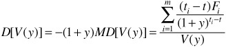
In practice, it is preferable to use futures contracts or swaps instead of bonds to hedge a bond portfolio because of significantly lower costs and higher liquidity. For example, using futures as hedging instruments, the hedge ratio φ_f is equal to

where N_F is the size of the futures contract. $dur_CTD is the $duration of the cheapest to deliver, and cf is the conversion factor.

Using standard swaps, the hedge ratio φ_s is

where N_S is the nominal amount of the swap, and $dur_S is the $duration of the fixed-coupon bond forming the fixed leg of the swap contract.⁴

Duration hedging is very simple. However, one should be aware that the method is based on the following, very restrictive assumptions:

• It is explicitly assumed that the value of the portfolio could be approximated by its first-order Taylor expansion. This assumption is all the more disputable that changes of the interest rates are larger. In other words, the method relies on the assumption of small yield-to-maturity changes. This is why the hedging portfolio should be readjusted reasonably often.

• It is also assumed that the yield-curve is only affected by parallel shifts. In other words, interest-rate risk simply is considered as a risk on the general level of interest rates.

In what follows, we attempt to relax both assumptions to account for more realistic changes in the term structure of interest rates.

RELAXING THE ASSUMPTION OF A SMALL SHIFT

We have argued that $duration provides a convenient way to estimate the impact of a small change dy in yield on the value of a bond or a portfolio.

Using a Second-Order Taylor Expansion

Duration hedging only works effectively for small yield changes because the price of a bond as a function of yield is nonlinear. In other words, the $duration of a bond changes as the yield changes. When a portfolio manager expects a potentially large shift in the term structure, a convexity term should be introduced, and the price change approximation can be improved if one can account for such nonlinearity by explicitly introducing the convexity term.

Let us take the following example to illustrate this point. We consider a 10-year maturity and 6% annual coupon bond trading at par. Its modified duration and convexity are equal to 7.36 and 57.95, respectively.⁵ We assume that the yield-to-maturity goes suddenly from 6% to 8%, and we reprice the bond after this large change. The new price of the bond, obtained by discounting its future cash-flows, is now equal to $86.58, and the exact change in value amounts to –$13.42 (= $86.58 – $100). Using a first-order Taylor expansion, the change in value is approximated by – $14.72 (= × $100 × 7.36 × 0.02), which overestimates the decrease in price by $1.30. We conclude that a first-order Taylor expansion does not provide us with a good approximation of the bond price change when the variation of its yield-to-maturity is large.

If a portfolio manager is concerned about the impact of a larger move dy on a bond portfolio value, one needs to use (at least) a second-order version of the Taylor expansion as given below.

where the quantity V′′ also denoted $conv[V(y)] is known as the $convexity of the bond V.

Dividing Eq. (48–8) by V(y), we obtain an approximation of the relative change in value of the portfolio as

where RC[V(y)] is called the (relative) convexity of portfolio V.

We now reconsider the preceding example and approximate the bond price change by using Eq. (48–8). The bond price change is now approximated by –$13.56 [= –14.72 + (100 × 57.95 × 0.02²/2)]. We conclude that the second-order approximation is better suited for larger interest-rate deviations.

Performing Duration/Convexity Hedging

Hedging by taking into consideration first and second orders is called duration/convexity hedging. To perform a duration/convexity hedge, a portfolio manager needs to introduce two hedging instruments. We denote the value of the two hedging instructions by H₁ and H₂. The goal is to obtain a portfolio that is both $duration-neutral and $convexity-neutral. The optimal quantity (φ₁, φ₂) of these two hedging instruments to hold is then given by the solution to a system of equations at each date, assuming that dy = dy₁ = dy₂. The system of equations consists of two equations and two unknowns and can be solved easily algebraically.

More formally, the sytem of equations is

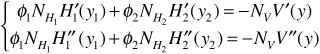
which can be rewritten as:

or

RELAXING THE ASSUMPTION OF A PARALLEL SHIFT

Duration and duration/convexity hedging are based on single-factor models because only one interest rate is being considered. In this section we look at how we can go beyond a single-factor model to a term-structure factor model.⁶

Accounting for the Presence of Multiple Risk Factors

A major shortcoming of single-factor models is that they imply that all possible zero-coupon rates are perfectly correlated, making bonds redundant assets. We know, however, that rates with different maturities do not always change in the same way. In particular, long-term rates tend to be less volatile than short-term rates. An empirical analysis of the dynamics of the interest-rate term structure suggests that two or three factors account for most of the yield-curve changes. They can be interpreted, respectively, as level, slope and curvature factors (see below). This strongly suggests that a term-structure factor model should be used for pricing and hedging fixed income securities.

There are different ways to generalize duration hedging to account for nonparallel deformations of the term structure. The common principle behind all techniques is the following. Going back to Eq. (48–1), let us express the value of the portfolio using the entire curve of zero-coupon rates, where we now make explicit the time dependency of the variables. Hence we consider V_t to be a function of the zero-coupon rates R(t, t_i – t). The risk factor is the yield-curve as a whole, a priori represented by m components, as opposed to a single variable, the yield-to-maturity y.

The main challenge is then to narrow down this number of factors in the least arbitrary way. The good news is that one can show that a limited number (two or three) of suitably designed risk factors can account for a large fraction of the information in the whole term yield-curve dynamics. There is actually a systematic method that allows us to achieve this very objective through what is known as a principal components analysis (PCA) of interest-rate changes, as will now be explained. This arguably has become the state-of-the-art technique for interest-rate risk management.

Regrouping Risk Factors through a Principal Component Analysis

The purpose of PCA is to explain the behavior of observed variables using a smaller set of unobserved, implied variables. From a mathematical standpoint, it consists of transforming a set of m correlated variables into a reduced set of orthogonal variables that reproduce the original information present in the correlation structure. This tool can yield interesting results, especially for the pricing and risk management of correlated positions. Using PCA with historical zero-coupon rate curves in major bond markets, it has been observed that the first three principal components of spot-curve changes, which can be interpreted as level, slope, and curvature factors, explain the main part of the returns variations on fixed income securities over time. More specifically, studies of spot rates in the U.S., German, Italian, French, Swiss, and Belgium government bond markets, found that at least 90% of the variation in returns can be explained by the three factors. The level component was the first factor which explained from 59% to 93% of the return variation. ⁷

Using a PCA of the yield-curve, we may now express the change dR(t, θ_k) = R(t + 1, θ_k) – R(t, θ_k) of zero-coupon rate R(t, θ_k) with maturity θ_k at date t as a function of changes in the principal components (unobserved implicit factors)

where c_lk is the sensitivity of the kth variable to the lth factor, defined as

which amounts to individually applying a, say, 1% variation to each factor and computing the absolute sensitivity of each zero-coupon yield-curve with respect to that unit variation.

These sensitivities are commonly called the principal component $durations. C_t^l is the value of the lth factor at date t, and ε_tk is the residual part of dR(t, θ_k) that is not explained by the factor model.

One can easily see why this method has become popular. Its main achievement is that it allows for the reduction of the number of risk factors with an optimally small loss of information. Since these three factors (parallel movement, slope oscillation, and curvature), regarded as risk factors, explain most of the variance in interest-rate changes, we may now use not more than three hedging instruments. We now write the changes of value of a fixed income portfolio as

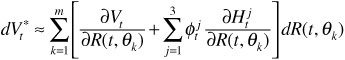
We then use to obtain

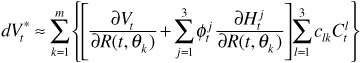
or

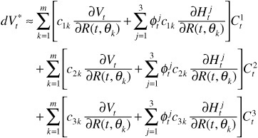
The first term in this expression is commonly called the principal component $duration of portfolio V^* with respect to factor 1.

If we want to set the (first order) variations of the hedged portfolio to zero for any possible change in interest rates dR(t, θ_k) or, equivalently, for any possible evolution of the terms, we may take as a sufficient condition, for l = 1, 2, 3,

This is a neutral principal component $durations objective.

Finally, on each possible date, we are left with three unknowns and three linear equations. Let us introduce the following matrix notation

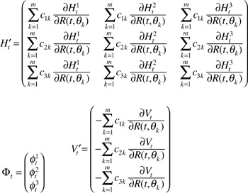
We then have the system

The solution is given by

In practice, one needs to estimate the principal components $durations used at date t. They are derived from a PCA performed on a period prior to t, for example, [t – 3 months, t]. As a result, the output of the method becomes strongly sample-dependent. In an attempt to alleviate this concern over robustness, it is actually more convenient to use a suitable functional specification for the zero-coupon yield-curve, provided that it is consistent with results from a PCA.

Hedging Using a Three-Factors Model of the Yield-Curve

The idea here consists of using a model for the zero-coupon rate function. We detail below the Nelson and Siegel model,⁸ as well as the Svensson (or extended Nelson and Siegel) model.⁹ One may alternatively use the Vasicek model,¹⁰ the extended Vasicek model, or the Cox-Ingersoll-Ross (CIR) model,¹¹ among many others.¹²

Nelson-Siegel and Svensson Models

Nelson and Siegel suggested modeling the continuously compounded zero-coupon rates R^c (0, θ) as

a functional form that was later extended by Svensson as

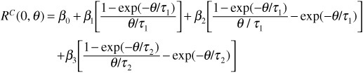
where

R^C(0, θ) = continuously compounded zero-coupon rate at time zero with maturity θ

β₀ = limit of R^C(0, θ) as θ goes to infinity (In practice, β₀ should be regarded as a long-term interest-rate.)

β₁ = limit of R^C(0, θ) – β₀ as θ goes to 0 (In practice, β₁ should be regarded as the short- to long-term spread.)

β₂, β₃ = curvature parameters

τ₁ and τ₂ are scale parameters that measure the rate at which the short- and medium-term components decay to zero.

As shown by Svensson, the extended form is a more flexible model for yield-curve estimation, in particular in the short-term end of the curve, because it allows for more complex shapes such as U-shaped and hump-shaped curves. The parameters β₀, β₁, β₂, and β₃ typically are estimated on a daily basis by using an ordinary least squares (OLS) optimization program, which consists, for a basket of bonds, of minimizing the sum of the squared spread between the market price and the theoretical price of the bond as obtained with the model.¹³

We can see that the evolution of the zero-coupon rate R^C(0,θ is entirely driven by the evolution of the beta parameters, the scale parameters being fixed.

In an attempt to hedge a bond, for example, one should design a global portfolio with the bond and hedging instrument so that the portfolio achieves a neutral sensitivity to each of the beta parameters. Before the method can be implemented, one therefore needs to compute the sensitivities of any arbitrary portfolio of bonds to each of the beta parameters.

Consider a bond that delivers principal or coupon and principal payments denoted by F_i at dates θ_i, for i = 1, . . . ,m. Its price P₀ at date t = 0 is given by the following formula:

In the Nelson and Siegel and Svensson models, we can calculate at date t = 0 the $durations D_i = ∂P₀/∂β _i for i = 0, 1, 2, 3 of the bond P to the parameters β₀, β₁, β₂, and β₃. They are given by the following formulas:^14,15

Hedging Method

The next step consists of creating a global portfolio that would be unaffected by (small) changes of parameters β₀, β₁, β₂, and β₃. This portfolio will be made of

• The bond portfolio to be hedged, whose price and face value are denoted by P and N_P

• Four hedging instruments, whose prices and face values are denoted by G_i and N_Gi, for i = 1, 2, 3, and 4

We therefore look for the quantities q₀, q₁, q₂, and q₃ to invest, respectively, in the four hedging instruments G₀, G₁, G₂ and G₃ so as to satisfy the following linear system:

In the Nelson and Siegel model, we only have three hedging instruments because there are only three parameters.

COMPARATIVE ANALYSIS OF VARIOUS HEDGING TECHNIQUES

We now analyze the hedging performance of three methods in the context of a specific bond portfolio. The methods we consider in this horse race are the duration hedge, the duration/convexity hedge, and the Nelson-Siegel $durations hedge.

Let us assume that at the initial date t = 0 the continuously compounded zero-coupon yield-curve is described by the following set of parameters of the Nelson and Siegel model¹⁶: β₀ = 8%, β₁ = –3%, β₂ = –1%, and τ = 3.

This corresponds to a standard upward-sloping yield-curve. We consider a bond portfolio whose features are summarized in Exhibit 48–1. The price is expressed in percentage of the face value, which is equal to $100 million. We compute the yield-to-maturity (YTM), the $duration, the $convexity, and the level, slope, and curvature $durations of the bond portfolio, as given by Eq. (48–10).

EXHIBIT 48–1
Characteristics of the Bond Portfolio to Be Hedged

To hedge the bond portfolio, we use three-plain vanilla six-month LIBOR swaps whose features are summarized in Exhibit 48–2. $duration, $convexity, level, slope, and curvature are those of the fixed-coupon bond contained in the swap. The principal amount of the swaps is $1 million. They all have an initial price of zero.

We consider that the bond portfolio and the swap instruments present the same default risk, so we are not concerned with this additional source of uncertainty, and we can use the same yield-curve to price them. This curve is the one described earlier with the Nelson and Siegel parameters.

To measure the performance of the three hedging methods, we assume 10 different possible changes in the yield-curve. These 10 scenarios are obtained by assuming the following changes in the beta parameters in the Nelson and Siegel model:

• Small parallel shifts with β₀ = +0.1% and β₀ = –0.1%

• Large parallel shifts with β₀ = +1% and β₀ = –1%

• Decrease and increase of the short- to long-term spread with β₁ = +1% and β₁ = –1%

• Curvature moves with β₂ = +0.6% and β₂ = –0.6%

• Flattening and steepening moves of the yield-curve with (β₀ = –0.4%, β₁ = +1.2%) and (β₀ = +0.4%, β₁ = –1.2%)

EXHIBIT 48–2
Characteristics of the Swap Instruments

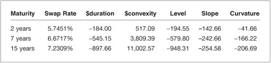
EXHIBIT 48–3
New Yield-Curve after an Increase (β₁ =+1%) and a Decrease (β₁ =–1%) of the Slope Factor

The six last scenarios, which represent nonparallel shifts, are displayed in Exhibits 48–3, 48–4, and 48–5.

Duration hedging is performed with the 7-year maturity swap using Eq. (48–7), leading us to enter 1,047 payer swaps. Duration/convexity is performed with the 7-year and 15-year maturity swaps using Eq. (48–9), leading us to enter 337 7-year maturity payer swaps and to enter 841 15-year maturity receiver swaps. Nelson and Siegel $durations hedge is performed with the three swaps using Eq. (48–11), leading us to enter 407 2-year maturity payer swaps, to enter 219 7-year maturity receiver swaps, and to enter 696 15-year maturity payer swaps. Results are given in Exhibit 48–6, where we display the change in value of the global portfolio (which aggregates the change in value on the bond portfolio and the hedging instruments), assuming that the yield-curve scenario occurs instantaneously. This change in value can be regarded as the hedging error for the strategy. It would be exactly zero for a perfect hedge.

EXHIBIT 48–4
New Yield-Curve after an Increase and a Decrease of the Curvature Factor (β₂ =+0.6%) and (β₂ =–0.6%)

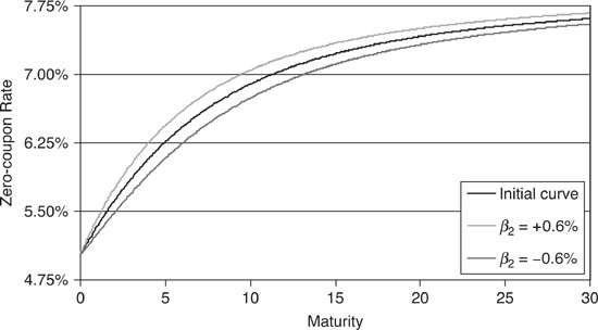
EXHIBIT 48–5
New Yield-Curve after a Flattening Movement (β₀ =–0.4%, β₁ = +1.2%) and a Steepening Movement (β₀ = +0.4%, β₁ =–1.2%)

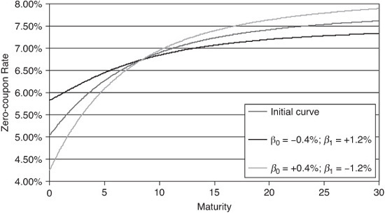
EXHIBIT 48–6
Hedging Errors in Dollars of the Three Different Methods: Duration, Duration/Convexity, and Nelson and Siegel $durations

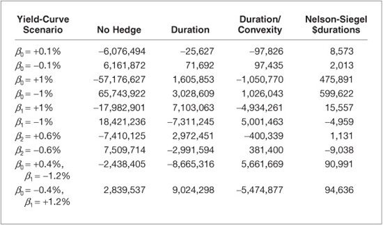
The value of the bond portfolio is equal to $972,375,756.¹⁷ With no hedge, we see clearly that the loss in portfolio value can be significant in all adverse scenarios.

As expected, duration hedging appears to be effective only for small parallel shifts of the yield-curve. The hedging error is positive for large parallel shifts because of the positive convexity of the portfolio. For nonparallel shifts, the loss incurred by the global portfolio can be very significant. For example, the portfolio value drops by $7,311,245 in the pure-slope scenario when β = –1% and $8,665,316 in the steepening scenario. As also expected, duration/convexity hedging is better than duration hedging when large parallel shifts occur. On the other hand, it appears to be ineffective for all other scenarios, even if the hedging errors are still better (smaller) than those obtained with duration hedging. Finally, we see that the Nelson and Siegel $durations hedging scheme is a very reliable method for all kinds of yield-curve scenarios. In all cases, the hedging error appears to be negligible when compared with the initial value of the bond portfolio.

KEY POINTS

• A decline (rise) in interest rates will cause a rise (decline) in bond prices.

• Just as the risk on a stock portfolio is usually proxied by its beta, which is a measure of the stock sensitivity to market movements, bond price risk is most often measured in terms of the bond interest-rate sensitivity, or duration. This is a convenient one-dimensional measure of the bond’s sensitivity to interest-rate movements.

• Duration provides a portfolio manager with a convenient hedging strategy: to offset the risks related to a small change in the level of the yield-curve, a portfolio manager should optimally invest in a hedging asset a proportion equal to the opposite of the ratio of the (dollar) duration of the bond portfolio to be hedged by the (dollar) duration of the hedging instrument.

• Duration hedging is convenient because it is very simple. However, it is based on the following very restrictive assumptions: (1) changes in the yield curve will be small, and (2) the yield curve is only affected by parallel shifts.

• An empirical analysis of major government bond markets suggests, however, that large variations can affect the yield-to-maturity curve and that three main factors (level, slope, and curvature) have been found to drive the dynamics of the yield-curve. This strongly suggests that duration hedging is inefficient in many circumstances.

• By relaxing the two assumptions for duration hedging, better methodologies for hedging can be developed.

• Relaxing the assumption of a small change in the yield-curve can be performed though the introduction of a convexity adjustment in the procedure. Convexity is a measure of the sensitivity of dollar duration with respect to yield changes.

• Accounting for general, nonparallel deformations of the term structure is not easy because it increases the dimensionality of the problem.

• Because it is never easy to hedge the risk associated with too many sources of uncertainty, it is always desirable to try to reduce the number of risk factors and identify a limited number of common factors. This can be done in a systematic way by using an appropriate statistical analysis of the yield-curve dynamics. Alternatively, one may choose to use a model for the discount-rate function.