
CHAPTER
FIFTY-FOUR
FIXED INCOME TRANSITION MANAGEMENT
Managing Director
BlackRock
DANIEL GALLEGOS
Director
BlackRock
Investing is a dynamic process. Portfolios shift over time, as a result of market movement or investment changes. Transition management refers to the process by which institutional portfolios are efficiently and cost-effectively reallocated.
Moving from the current allocation to the desired allocation presents a risk/cost tradeoff similar to the risk/return tradeoff familiar in investment management. In this way, portfolio transitions closely resemble short-term investment assignments. Transition management focuses on identifying and implementing a strategy to arrive at the target portfolio most efficiently, given the investor’s risk/cost priorities.
Transitions can be triggered by a variety of events, most commonly changes in fund management (such as replacing a poorly performing investment manager), shifts in asset allocation (equity to fixed income), investment style (index to active), and benchmark universe (S&P 500 to Russell 1000).1 Transitions range in complexity from a straightforward liquidation of fund assets to a complete portfolio restructuring encompassing multiple asset classes and countries.
Historically, transitions were often viewed as an operational issue, a secondary consequence of a larger investment decision. It was not uncommon for the fiduciary to direct the previous investment manager to liquidate the original (legacy) portfolio and have the new manager invest the cash proceeds in the desired (target) portfolio, thereby incurring round-trip transaction costs. Greater awareness of transaction costs, together with concerns about fiduciary responsibilities, has led institutional investors to increasingly use transition managers for portfolio restructurings.2
Yet, despite the importance of portfolio transitions, many investment professionals do not fully understand the complexities involved. Indeed, some transitions can experience significant volatility of outcomes in the space of a few days. This is especially important, as we explain below, for fixed income transitions where assets are often illiquid and markets are opaque. In this chapter, we explain the process of transition management and the appropriate balance of portfolio risk and transaction costs. We introduce cost and risk measures, discuss the unique features of fixed income transitions, and illustrate several of these factors in a case study.
BASICS OF FIXED INCOME TRANSITIONS
Before turning to a more in-depth consideration of risk and cost, it is worth outlining the basics of transition management, including a chronology of events, the types of risk that must be managed for all transitions (regardless of asset class), and a discussion of what makes fixed income transitions unique.
Chronology of Transition Events
The fixed income transition management process is made up of various distinct phases: manager selection, communication of objectives, determination of trade list, pre-trade analysis, creation of trade strategy, execution, and post-trade reporting. A description of these phases and their importance to the overall event are provided below.
1. Manager selection: After the decision to use a transition manager is made, the fiduciary or plan sponsor undertakes a due diligence process to select the manager. Investors typically seek the same level of market expertise, risk management, liquidity, operational infrastructure, and fiduciary oversight during transitions that they have come to expect from asset managers. Transitions that are not properly managed can result in significant underperformance and excessive fee-taking. Managers can be broker-dealers, custodians, or specialized transition managers; they vary in terms of their access to liquidity, trading skill, and risk control. Successful transition managers actively mitigate transition risk by minimizing market impact and opportunity cost during trading, and by carefully controlling transaction costs such as commissions and spreads.
2. Communication of objectives: The transition manager must understand the client’s motivation and desired timing for the transition, as well as their tolerance for risk and cost. The client may also have benchmark preferences for measuring cost (previous closing price, volume-weighted average price, etc.). Other factors that could affect the transition are also communicated to the transition manager at this time (regulatory prohibitions against internal crossing, among others).
3. Determination of trade list: Having established the legacy and target portfolios, the manager determines the common holdings that can be transferred in-kind between them (meaning that the underlying securities retained for the target portfolio are transferred directly, cost and risk free, rather than liquidated). The remainder must be traded. Essential operational steps and necessary legal and administrative issues also must be resolved at this point.
4. Pre-trade analysis: The manager uses pre-trade analytical models to assess the liquidity characteristics of the trade list (focusing on breakdowns by side, order size, sector, industry, country, etc.) and estimate total portfolio trading costs and likely variation in those costs. Managers also use risk models, typically fundamental multifactor models, to estimate the tracking error between the legacy and target portfolios.
5. Creation of trading strategy: Strategies can vary widely in terms of aggressiveness and complexity. A common strategy is simply to trade a constant fraction of the list over the transition, with the objective of executing at the volume-weighted average price (VWAP) for the period. In some cases, managers may use optimization tools to determine the dynamic trading strategy most appropriate for the transition. The transition duration, cost estimate, and dispersion in outcomes are communicated to the client before the transition begins, to form an objective benchmark for measuring the eventual outcome of the transition.
6. Execution: The manager then executes the trades in a manner consistent with the strategy formulated in the previous step, while also making adjustments necessitated by changing market conditions. Actual transitions can range in duration from a single day to over a month, depending on the client’s objectives and complexity of the trades.
7. Post-trade reporting: The manager provides a detailed report to the client, with particular attention to the realized costs (including commissions, bid/ask spreads, and market impact costs) relative to the pre-trade estimate. It is important to note that transition performance is measured from the date on which the transition manager is able to start executing the restructuring (as opposed to the client’s decision date) to truly reflect the transition manager’s efforts.
Types of Transition Risk
A poorly managed portfolio restructuring—one that does not assess and address all risks properly—has the potential to erase an entire year of investment returns. There are four types of risk that must be managed across all transitions:
• Exposure Risk: Also known as investment risk, exposure risk is associated with factors that can have a negative effect on portfolio value. Transition managers use a variety of processes (various types of trade analytics), tools (portfolio optimizers, for example), and market expertise (including broker-dealer relationships) to help minimize exposure risk.
• Execution Risk: After the transition strategy has been set, there is still risk of implementing the plan with suboptimal results, particularly for illiquid asset classes. Key to sourcing liquidity is understanding the intrinsic value and structural nuances of each security being traded.
• Process Risk: Communication gaps and unchecked assumptions contribute to process risk, which results in additional transition costs. Rigorous and detailed methodology helps minimize this risk.
• Operational Risk: This is the risk that operational details, such as account setup and reconciliation, are overlooked or delayed. Transition managers create transparent and auditable reporting to reduce this possibility.
Each type of risk should be managed comprehensively throughout every transition. For fixed income portfolios in particular, there are several market factors—discussed below—that make these transitions especially challenging.
Uniqueness of Fixed Income Transitions
The nature of fixed income securities makes transitions involving this asset class rather unique relative to those of other asset classes, especially equities. Several factors are particularly relevant here in terms of cost and risk:
• Market Structure: Fixed income securities are typically not traded on an open exchange, so pricing lacks uniformity and transparency.3 Varied maturities, volatility due to interest rate instability, nuances in investment characteristics, and currency fluctuations pose significant challenges for fixed income portfolio transitions, which are well beyond the scope of most equity transitions. In terms of the framework above, the absence of last trade reporting (e.g., a ticker tape for most fixed income securities) makes it very difficult to measure actual costs using the shortfall framework, let alone make accurate estimates before the transition begins.
• Price Discovery and Liquidity: Market structure and the complexity of instruments also affect the trading strategy and execution. Unlike equities, price discovery and liquidity sourcing are particularly critical for fixed income transitions. The absence of a single, centralized bond exchange and the proliferation of instruments necessitate the use of available sources of liquidity to achieve best execution. Thus, transition managers actively pursue counterparties across multiple platforms. Transition managers benefit from long-standing relationships with broker-dealers around the world to maximize trading opportunity and achieve better execution.
• Types of Exposure Risk: It is difficult to gauge the active risk (tracking error) of a complex bond portfolio and, hence, to implement an optimal trading strategy, as discussed above. The typical fixed income transition may be subject to multiple dimensions of risk, including:
• Rate risk
• Volatility risk
• Credit-spread risk
• Idiosyncratic risk
Fixed income transition managers develop and implement techniques, metrics, and reporting tools specific to fixed income securities that are designed to achieve the investors’ target portfolio with the lowest risk possible.
TRANSITION METRICS AND OBJECTIVES
With an understanding of the challenges specific to fixed income transitions, we can now turn our attention to an in-depth discussion of risk and cost. A variety of metrics for cost and risk are commonly used to measure the performance of a transition. In this chapter, we focus on implementation shortfall and tracking error. The first, implementation shortfall, measures the amount by which the legacy portfolio’s return falls short of the target portfolio’s return. This metric allows an investor to evaluate how their portfolio performed during the restructuring period. The expected implementation shortfall is established prior to the transition and decomposed into return factors, when the transition manager formulates the restructuring strategy.
For similar insights, we focus on risk in terms of portfolio tracking error (TE), which refers to the absolute difference between the returns of the legacy and target portfolios. With these metrics in hand, we then formally define the transition manager’s objective.
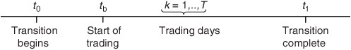
To illustrate why these measures are most appropriate, a more formal statement is useful. Let N denote the number of assets in the universe defined by the union of the legacy and target portfolios, and let Ω denote the N × N variance-covariance matrix of asset returns. From the viewpoint of the transition manager, the process begins on day t0 when the transition manager is first in a position to begin trading the legacy portfolio.4 We denote by V0 the initial value of the portfolio at this date. Trading need not occur immediately. For example, transition managers might postpone trading to source liquidity or unexpected delays might arise. At calendar time tb (where t0 ≤ tb), the manager actually begins executing the transition through trading. Let T denote the duration of the transition, which we think of as days but could also represent hours or other intraday periods. Trading occurs in waves on each day (indexed by k = 1,…, T), and the transition is completed on day t1 = t0 + T. The timeline for the transition is illustrated in Exhibit 54–1.
EXHIBIT 54–1
Transition Timeline
Denote by L the N × 1 vector of asset holdings of the legacy portfolio, where each row represents the shares held of the asset, and similarly define by Q the holdings in the target portfolio. We denote by hL and hQ the corresponding vectors of holdings (weights) in the legacy and target portfolios, where the i-th element of the holding vector represents the portfolio weight in asset i as a fraction of total portfolio value.
Active risk is defined as the distance between the legacy and target portfolios, captured as
![]()
Note that when the transition is a straight liquidation to cash, we have hQ = 0, the null vector, and the active risk is simply the standard deviation of the legacy portfolio; that is, ![]() . Similarly, when the transition is a cash investment, hL = 0, and the active risk is the standard deviation of the target portfolio,
. Similarly, when the transition is a cash investment, hL = 0, and the active risk is the standard deviation of the target portfolio, ![]() . Thus, the active risk for non-rebalance transitions (either into or out of cash) will typically be higher than for transitions in which at least some holdings are in common.
. Thus, the active risk for non-rebalance transitions (either into or out of cash) will typically be higher than for transitions in which at least some holdings are in common.
Defining Transition Costs
The trade list is simply the N × 1 vector of shares,
![]()
with the convention that positive elements represent purchases and negative elements represent sales.
Total transaction costs incorporate explicit costs (commissions, taxes, and fees) and implicit costs (bid/ask spreads, market impact).5 In a transition, unlike most institutional trading, orders are (nearly) always completed, so opportunity costs from failing to execute generally are not a factor.6 In keeping with previous research, costs are expressed relative to the pre-trade benchmark (strike) price. Formally, for asset i = 1,…, N, the realized transaction cost is
where
Dates k 1,…, N,
![]() , is the execution price,
, is the execution price,
xi,k is the signed trade size,
φi,k represents the explicit trading cost (with the sign convention that costs are positive for buys and negative for sells), and
![]() is the benchmark or strike price against which costs are measured.
is the benchmark or strike price against which costs are measured.
For purchases, we expect costs to be positive; for sales, the figure should be negative. Dollar implementation shortfall is the total cost measured relative to a benchmark price struck at time tb is ![]() . Throughout this chapter, we use implementation shortfall to refer to the total realized costs relative to initial transition value C(tb) = C(tb)/V0.
. Throughout this chapter, we use implementation shortfall to refer to the total realized costs relative to initial transition value C(tb) = C(tb)/V0.
The return of the target portfolio over the period of the transition (from t0 to t1) is denoted rQ (t0, t1); this is the return earned by an investor who already held the target portfolio at the beginning of the transition. The actual return of the legacy (restructured) portfolio from t0 to t1 is defined as
![]()
The final value of the legacy portfolio once the transition is complete is the end of period share holdings (L + X) evaluated at prices at the end of the transition, less the net cash-flows from trading. Using the definition of costs, it is straightforward to show that
![]()
where c(tb) is the total implicit and explicit trading cost as a fraction of portfolio value (given a benchmark struck just prior to trading), and rL(t0,tb) is the return on the legacy portfolio from the time the transition began, a timing cost. In cases in which the transition begins without delay, the benchmark price is struck at time t0, so ![]() and we see that the implementation shortfall cost is the difference between the actual return of the transition (legacy) account compared with the return on the target fund, had the transition been implemented instantaneously at no cost. This explanation shows why implementation shortfall is the right measure of costs. It accurately captures the slippage between the legacy and target portfolios, reflecting all costs incurred during the transition.7
and we see that the implementation shortfall cost is the difference between the actual return of the transition (legacy) account compared with the return on the target fund, had the transition been implemented instantaneously at no cost. This explanation shows why implementation shortfall is the right measure of costs. It accurately captures the slippage between the legacy and target portfolios, reflecting all costs incurred during the transition.7
Transition Tradeoffs
Having defined formally both risk and cost, we can now specify possible transition objective functions. As mentioned above, the transition manager and client jointly determine the trading strategy with the client’s objectives in mind. Typically this involves a tradeoff between cost and active risk. Formally, predicated upon a horizon of T trading days, the optimal transition strategy can be defined as the set of trading waves that minimize, in expectation, a convex combination of c(tb) and σL,Q, with weight λ. Formally,
![]()
subject to
ΣXk = X
Both cost and risk depend on the particular waves chosen. For example, if λ is very high and the trading strategy is very aggressive, the bulk of the trade list may be completed in the first or second wave (recall, there could be multiple waves in a day), which might lead to high trading impact but low tracking error.
What is the optimal solution to this objective? Various heuristics are commonly employed but often fail to actually minimize costs. Some managers believe that maximizing the crossing rate will always minimize market impact and, hence, costs. However, this fails to account for the additional risk caused by prolonging the transition, which is a common problem in many fixed income securities in which crossing is a low-probability event. Another common strategy (usually referred to as the VWAP strategy because it is associated with a trading benchmark of the volume-weighted average price) is simply Xt = X/T, where the order is broken up equally over time. The VWAP strategy may not, however, be the optimal solution (even if λ = 0) and it may not minimize costs.
Rather, the optimal solution can be found using stochastic dynamic programming, given assumptions about the evolution of prices and liquidity. This forward-looking approach is based on the idea that the solution (or policy function) at any point throughout the trading session k, must still be optimal for the remaining program.8 Using a forward-looking approach also allows the transition manager to capture variations in liquidity or volatility (the key drivers of cost) that are known to occur over the period of the transition. For example, a transition executed during a period with highly anticipated macroeconomic events (e.g., earnings season) can take into account likely spikes in volatility and volume. This approach can also provide a tradeoff between cost and risk for various λ, allowing the client to visualize the alternatives. The dynamic programming approach requires a considerable degree of confidence in the input estimates, which may not always be the case for less liquid assets. In those cases, the transition manager can use their experience and judgment (sometimes guided by the formal analysis) to correctly sequence the trades in accordance with client objectives. Whether the strategy is specified formally or informally, however, the basic tradeoffs outlined above are present in every transition.
Implementation Shortfall Example
To illustrate the concepts above, consider a $1 billion international equity transition. A state retirement system sought to rebalance its international positions by reallocating the legacy portfolio to two new managers. The total transition period was eight days, of which the trading period was five days. Forecast costs for the trade list were 0.51%. The transition manager used proprietary analytical tools to match and split out buys and sells, then utilized a transaction cost model to predict the (half) bid/offer spread plus estimated market impact. The manager then added estimated commissions, fees, and taxes to this figure to determine the total forecast cost, which became the benchmark for evaluating the transition. Annualized active risk (i.e., the tracking error between the legacy and target portfolio) was 3.50%. Based on this figure, the estimated risk over the trading period was 0.39% (with 250 trading days annually, 0.495% = 3.5% ![]() . This figure was used to determine upper and lower bounds for the transition shortfall.
. This figure was used to determine upper and lower bounds for the transition shortfall.
Ex post, the actual average active risk was 0.38%, implying that the manager traded more aggressively to reduce the risk in the early stages of the transition. The legacy portfolio performance over this period was 0.69%, while the target portfolio returned 1.40% over the transition; applying Eq. (54–4) yields a total implementation shortfall of 0.71% (1.40%−0.69%). The realized trading shortfall was 0.58% (market impact of 0.42% and commissions and fees of 0.16%), in line with the pre-trade forecast. Timing costs accounted for 0.14%, reflecting outperformance of the target portfolio relative to the legacy portfolio in the three days before trading started.9 Overall, although total costs were slightly higher than predicted (7 bps), the outcome was within the range of possible outcomes communicated to the client before the transition, which signifies the success of this transition.
The Risk/Cost Tradeoff Revisited
Fixed income and equity market transitions are similar in terms of the risk/cost tradeoff outlined above, but there are material differences in how these transitions are executed. Like most U.S. equities, the majority of investment-grade debt can be liquidated or purchased within a short period of time. However, additional costs are normally incurred when selling or buying too quickly. Conversely, executing too slowly will extend the restructuring timeline and expose assets to the increased risk of implementation shortfall. Either scenario can have material impact on the cost and quality of the restructuring. It is a transition manager’s job to evaluate each portfolio constituent and the expected risk/cost tradeoff in order to design and implement a suitable restructuring strategy, while satisfying the client’s timing objectives.
Implementation Issues Specific to Fixed Income
The optimal fixed income transition strategy addresses various concerns:
• Sector misweights
• Term-structure profile differences
• Illiquid securities
• Timing preferences
Although many of these are common portfolio characteristics, it is crucial to implement a strategy that will decrease the costs associated with portfolio-specific nuances across these parameters. Another of the transition manager’s responsibilities is to dissect structural differences between the target and legacy portfolios and then create an optimized transition strategy that will mitigate risks born of those structural differences.
Evaluating Liquidity Sources
Managers must evaluate the many details of each fixed income security to identify the correct liquidity source. Common descriptive data points such as coupon type, maturity, subordinate structure, and issuer are reviewed and logged. There may be numerous issues with various structures, and each issuance may be brought to market by different banking syndicates. For example, there are nearly 30 different corporate bonds listed for IBM, with various terms to maturity and coupon types, as opposed to just one equity security. And this is only for one type of fixed income security. Legacy portfolios may hold many different types of securities (mortgage-backed securities, Treasuries, corporates, munis, etc.). The diverse array of security types makes it increasingly complex to identify the correct liquidity sources for each asset during a restructuring. To effectively evaluate liquidity sources, a trading desk must have expertise across the various markets and security types. Trade research teams can also help identify trading bottlenecks, optimal execution dates and preferred trading counterparties.
Using Derivatives to Manage Risk or Lower Cost
Derivatives can play an important role in fixed income transition management, particularly when liquidity is hindered and formidable differences exist between the legacy and target portfolios’ risk characteristics. Since decreasing the performance difference between a legacy and target portfolio is paramount when minimizing implementation shortfall, the ability to quickly and inexpensively restructure the risk characteristics of a portfolio is key.
Derivatives are commonly used during transitions to alter the legacy portfolio’s duration. They are an especially important tool when the liquidity timeline of the legacy portfolio is expected to be slow. U.S. Treasury futures contracts have proved particularly useful during transitions: They can be entered into quickly, in large notional sizes, with little or no market impact, and with minimal funding. Derivatives are also used to address sector misweights during a restructuring.
In situations in which operational and legal hurdles make derivatives less efficient, exchange-traded funds (ETFs) may be a more effective option, particularly when beta exposure is desired prior to selecting the target manager. Investors can achieve a diversified sector exposure using ETFs without increasing idiosyncratic risk, which can be associated with large volumes of cash securities.
CASE STUDY OF RISK MANAGEMENT
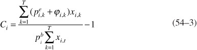
Having established the framework for transition management, we turn to a case study that illustrates some of the risk factors described above and the role that derivatives can play to reduce risk during a transition. An investment committee decided to shift the duration of a $100 million U.S. Treasury portfolio in its defined benefit plan, moving from exposure at the middle of the maturity curve to a concentration at the short and long ends of the curve. The legacy portfolio is benchmarked to a 7–10 year index; the target portfolio has more of a barbell shape, roughly 60% at the 1–3 year range and 40% at the 20+ year range. Despite the very different compositions, both portfolios have the same weighted-average duration (7.26 years).
There is, however, a mismatch in key rate duration between the two portfolios, or how sensitive each component is to changes in interest rates (Exhibit 54–2). This mismatch could translate into significant risk, even over the course of just one trading day. Consider the impact an abrupt increase in rates at the 15-year point could have had on this portfolio during a transition (Exhibit 54–3).
EXHIBIT 54–2
Key Rate Durations
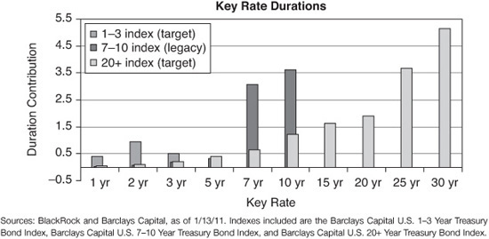
EXHIBIT 54–3
Impact of Interest-Rate Shock on 1/13/11
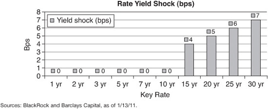
Price changes range from $0.51 (or 4 bps of yield) on the 15-year bond to $1.10 (or 7 bps of yield) on the 30-year bond. Given the asymmetric nature of bond prices, it is typical to see higher price dispersion at the long end of the yield-curve. Analyzing the portfolio in terms of its key rate duration helps identify where risk resides on the maturity curve.
In this interest rate shock environment, the difference between the two portfolios’ term structure profiles created a tracking error valued at $310,000. Approximately 10% of the expected annualized yield was at risk for this single restructuring.
The strategy for this transition focused on managing the portfolio’s key rate risk. The night before the 7–10 year holdings began to trade, futures contracts were bought and sold to rebalance the legacy portfolio’s key rate duration profile and better match the profile of the target portfolio. All five contracts were either bought or sold, decreasing exposure at the belly of the curve and increasing exposure at the long end. This single transition almost completely mitigated the mismatch in expected return between the portfolios; annualized active risk shrank from 491 to 24 bps.
As the 7–10 year trades were completed, the futures contracts were unwound and proceeds were used to purchase the target constituents.
Had the transition strategy focused on weighted-average duration—instead of key rate duration—the long bond risk would have been masked and the portfolio would have been vulnerable to price changes from the steepening rate curve.
Even though both the legacy and target portfolios held only U.S Treasuries (which carry neither credit-spread nor idiosyncratic risk) significant value was at risk in this portfolio restructuring. Fixed income transitions typically involve more than just a shift in Treasury duration, which means a heightened need for analytics and process that protect portfolio value throughout each restructuring.
KEY POINTS
• Transition management is the process of restructuring a portfolio in a way that optimizes the risk/cost tradeoff.
• Fixed income transitions are often complicated and potentially costly. The fixed income market structure offers less transparency and is more demanding in terms of identifying and evaluating liquidity; the diverse types of instruments presents additional trading challenges and varied risk factors (compared with equities).
• Because normal market volatility can put a large amount of the expected annualized return of a fixed income portfolio at risk during a transition, the ability to systematically manage the transition is imperative.
• Two metrics in particular can help investors evaluate their restructuring. Tracking error measures the level of active risk for the portfolio. Implementation shortfall gauges how a portfolio performed during the restructuring period.
• Derivatives are an important tool for managing risk and cost for fixed income transitions. They can be entered into quickly, in large notional sizes, with little or no market impact, and with minimal funding.