CHAPTER
SIXTY-SEVEN
CREDIT DERIVATIVE VALUATION AND RISK

DOMINIC O’KANE, D.PHIL. (OXON)

Affiliated Professor of Finance
EDHEC Business School

The purpose of this chapter is to set out the valuation methodology for credit swaps (CDS) and CDS indices. As described in Chapter 66, a credit default swap (CDS) is the most commonly traded credit derivative contract. It is also the building block for the CDS indices. An understanding of the valuation and risk management of CDS is therefore essential if we are to understand the valuation and risk management of CDS indices and other credit derivatives.

CDS VALUATION

For valuation purposes the essential features of a CDS contract are as follows:

• A regular fixed coupon is paid on the premium leg from the protection buyer to the protection seller according to a frequency and basis convention as set out in Exhibit 67–1. The coupon is paid until contract maturity date or a credit event, whichever occurs first. If the credit event occurs between two coupon payment dates, the market standard convention is that the portion of the coupon that had accrued from the previous payment date until the Event Determination Date¹ must be paid by the protection buyer.

EXHIBIT 67–1
Standard CDS Contract Specifications for North American and European Markets

• A payment of par minus the recovery rate is paid following a credit event. The recovery rate is set at the auction (which was described in Chapter 66) and paid shortly after on the auction settlement date.

We therefore have future cash flows which are contingent on a credit event. The CDS value is given by the expected present value of these flows calculated in the “risk-neutral” measure (i.e., using probabilities of a credit event that exactly reprice the term structure of market prices of quoted CDS).

The precise rules which generate the schedule of premium leg payments are listed in Exhibit 67–1. The CDS dates referred to in this Exhibit are March 20, June 20, September 20, and December 20.

Need for a Model

The pricing and risk management of a CDS contract requires the use of a pricing model. There are a number of reasons for this:

1. The CDS market is OTC. As such, there is no central location where trades are executed from which prices can be instantly reported. Prices are instead agreed bilaterally and privately. Market pricing providers such as Markit² only provide end-of-day pricing based on aggregating pricing submissions from various dealers.

2. Even if CDS contracts were exchange-traded, the quotation of prices would be complicated by the fact that there are so many different variations in the contracts outstanding. Consider just those contracts written against a single reference entity and assume that the longest maturity contract is 10 years and that all contracts trade with the same coupon and credit events. Since maturity dates are on a quarterly schedule, we can have as many as 40 different contracts being traded, albeit with varying degrees of liquidity. Quoting so many numbers per issuer can be cumbersome. A model that allows pricing based on a smaller number of market inputs is certainly preferable.

3. Although there is the concept of a standard CDS contract, market participants can request customized features which may deviate from this standard. For example, a company may wish to buy a forward CDS contract in which protection starts at some future date. To price this correctly relative to other CDS, a model is required that must also reprice the current market prices.

4. A valuation model is also important for risk management. With bonds, we need, at the very least, to introduce the concept of a yield-to-maturity and yield-curve before we can start to hedge the interest rate risk of a bond portfolio with other bonds. The same is true with a portfolio of credit default swaps. A model is needed in order to be able to quantify spread risk and to hedge the credit risk sensitivity of one CDS against another.

The value of a CDS contract is simply the upfront value at which the CDS contract should trade. For a protection seller, this is equal to the expected present value of the incoming coupons on the premium leg minus the expected present value of the protection leg. For a protection buyer, it is the negative of this since the protection buyer is receiving the protection but paying the coupons.

Even without a model, we can begin to think about the factors that affect the CDS value. We consider the two legs separately:

1. The value of the premium leg is the expected present value of the coupons paid until maturity or a credit event, whichever happens first. If the credit quality of the reference credit falls then this will make an early credit event more likely and so it is more likely that not all of the coupons will be received. The expected present value of the premium leg will then fall. Also, as it is an annuity of fixed coupons, its present value will also fall if interest rates rise. The value of the premium leg also increases with CDS maturity since more coupons are to be paid.

2. The value of the protection leg increases if the credit deteriorates since it becomes more likely that the payment of par minus the recovery rate will be received. It will also increase with increasing contract maturity as protection for a longer period is always more valuable than for a shorter period. However, it falls as interest rates increase since it is the present value of a future contingent payment.

Before we move on to describe a model that can value each of the legs, we first wish to show that it is possible to actually determine the no-arbitrage value of the upfront cost of protection by reference to the cash bond market.

THE CDS–BOND RELATIONSHIP

Subject to a number of important assumptions, there is a fundamental no-arbitrage relationship between the upfront value of a CDS and the price of a specific floating rate bond issued by the same reference entity. Specifically, our aim is to show that there is an exact relationship between the upfront cost of a time T maturity CDS, U, and the price P of a floating rate note with a time T maturity where the floating rate note pays a floating rate coupon equal to LIBOR plus a spread C. This spread must be equal to the fixed spread of the CDS. We need to consider the following trading strategy:

1. At time zero, an investor borrows an amount P + U at a funding rate of LIBOR. This assumes that the investor has a credit quality similar to that of highly rated commercial banks. This funding is locked in until future time T. Interest payments are made quarterly.

2. At time zero, the investor uses P of the borrowed money to buy one unit of face value of a time T maturity floating rate note issued by the reference entity at a specific seniority. The full price of this bond is P. For simplicity we assume that the purchase begins on a coupon payment date so that there is no accrued interest to consider.

3. At the same time, the investor uses U of the borrowed money to buy CDS protection on one unit of face value of the reference entity that matures at future time T. Note that U can be positive or negative. Following this, the now hedged investor will have to make quarterly coupon payments.

To analyze this strategy, we need to determine the payments at four different types of event: (1) initiation, (2) coupon payment dates, (3) following a credit event, and (4) maturity time T (assuming that no credit event has occurred). These are shown in Exhibit 67–2.

EXHIBIT 67–2
No-Arbitrage Strategy of Bond plus CDS Protection

For simplicity we assumed that the credit event occurs on a coupon payment date so that the repayment of the funding simply costs par, i.e., the face value of the borrowing, which in this case is (P + U), and so that there is no coupon accrued to be paid on the CDS.

As the initial net cash-flow is zero—the strategy costs nothing to enter—the expected value of the future payments should equal zero. For this to be true, we require that P + U = 100%, i.e., there is a fundamental no-arbitrage relationship between the upfront cost of the CDS and the price of a floating rate note issued by the same reference entity. For example, if the LIBOR floater is priced at par, then the upfront value is zero. However if the LIBOR floater is worth more than par, then the upfront cost of protection is negative. If the LIBOR floater is worth less than par, then the upfront cost of protection is positive.

In order to establish this relationship, we have had to make a number of simplifying assumptions. The main ones are:

1. We assumed that the bond buyer funded at LIBOR flat and that funding at this level can be locked in until the maturity of the CDS. In practice, the funding of the bond will be done in the repo market where it will generally not be possible to lock-in the funding level for any extended period. The hedged investor therefore has funding risk, which can work for or against them. There may also be a haircut on the amount funded and this depends on the market risk of the bond, which is used as collateral in the repo.

2. We assumed the existence of a T-maturity pari passu floater, which pays LIBOR plus C where C is equal to the fixed spread of the CDS contract.

3. We ignored the effect of the delivery option, which could allow the protection buyer to deliver a cheaper bond (if one exists). This is most likely to be of value if the CDS includes restructuring as a credit event. The value of this option should make the cost of protection higher.

4. We assumed that the credit event falls on a coupon payment date. In practice a default between coupon payment dates will mean an additional payment by the protection buyer of the accrued coupon on the CDS. For the bond, it may mean that the unpaid coupons are added to the bondholders’ claim in bankruptcy.

5. We ignored the effect of counterparty risk on the CDS. Counterparty risk is typically mitigated by the posting of upfront collateral.

6. We ignored tax effects that may treat the coupon and principal differently.

7. We ignored transaction costs and market technical effects. In the latter case, we note that since the CDS market makes it easier to short credit risk, any negative news on a credit will typically impact the CDS market first, causing the CDS upfront price to increase before bond prices fall.

What we have done here is to establish a link between the upfront costs of CDS and the pricing of a specific bond issued by the same reference entity. However, in practice, this is not a viable way to price CDS contracts since it is almost certain that the required T-maturity pari passu floater, which pays a spread equal to the coupon on the CDS, does not exist. Also, the list of assumptions means that although there is a strong relationship between bond prices and CDS upfront costs, the relationship is not exact.

The CDS Basis

The difference between the cash and CDS market is known as the CDS basis. It is defined as

CDS Basis = CDS Par Spread – Bond LIBOR Spread

This is not an exact definition since there are various ways to quote the bond LIBOR spread.³ One LIBOR spread widely used by the market is the asset swap spread of a bond of the issuer with a similar maturity to the CDS, which is trading at a price close to par.

Trading the CDS basis has become a relative value strategy of a number of credit investors, in particular credit hedge funds. The aim of basis trading is to determine which of the assumptions listed above is driving the difference between CDS spreads and bond spreads and to take a view on whether these are correctly or incorrectly priced and liable to change.

The standard basis trade is the “negative basis trade” in which the investor buys the bond and buys protection. It is called a negative basis trade because the investor receives the bond spread and pays the CDS spread—the investor receives negative of the basis as defined above.

Valuation of an Existing Contract

Consider an investor who sells protection using a five-year CDS contract at time zero. The upfront cost, which is the amount paid in cash to enter the contract is U (0). In return, the investor receives a regular coupon C and we call the expected present value of this the value of the premium leg. He also has to pay the counterparty (1 − R) on the face value of the protection if there is a credit event between the effective date and the contract maturity time. The expected present value of payment is the value of the protection leg. We can therefore state that U (0) is the cost of this where

U(0) = V_Premium (0.5) − V_Protection (0.5)

This is at initiation. Subsequently, at time t, the value of the premium leg and protection legs will change as coupons are received, maturity approaches and the market’s view of the default risk of the reference credit changes. At this time the value of the contract is given by

U(t) = V_Premium (t, 5) − V_Protection (t, 5)

One year later, the investor wishes to unwind his position. Given that he sold protection, he must now buy protection. The cost of entering into the long protection position is given by –U(1) where

U(1) = V_Premium (1, 5) − V_Protection (1, 5)

Since the coupon dates and any contingent protection payments on this new contract match exactly the coupon payment dates and any contingent protection payment on the existing contract, the combined position has future cash flows equal to zero. The mark-to-market value of this short protection CDS position at any time is therefore simply the upfront cost of buying protection to the same maturity as the initial contract. This is different from the P&L which is the money earned or lost by first selling protection and then closing out the trade one year later by buying protection. This is equal to the upfront cost U(1) which was received plus all of the rolled-up coupon payments minus the cost of repaying any initial loan U(0).

Market Pricing

The pricing of CDS is done with reference to the spreads at which the current market standard contracts trade. These are for contracts which terminate at the main maturity points, which include six-months and one, two, three, four, five, seven, and 10 years. The market has two conventions for quoting spreads. They are:

1. Par Spreads: The T-year par spread is defined as the coupon that would be paid for protection on a T-year contract which has no initial cost.

2. Flat Quoted Spread: The T-year flat quoted spread is defined as the level at which a flat CDS par spread curve needs to be marked in order that the model-implied upfront value matches the upfront value quoted in the market. It therefore ignores the shape of the term structure of the CDS market—it is the CDS equivalent of the bond yield-to-maturity.

The par spread was the quotation convention for the CDS market until 2010. The “problem” with the par spread is that calculation of the upfront value requires knowledge of the full term structure of par spreads of quoted CDS contracts with the same or shorter maturities. Therefore, several par spreads may be needed to calculate one CDS upfront value and one CDS upfront value cannot be used to imply a term structure of par spreads. As a result, the quoted flat spread has become the market standard. Its existence is based on a need to have a spread-based quotation for the price of a CDS contract. Use of the quoted flat spread also entails using the market standard recovery rate assumption, which is currently set at 40% for senior unsecured debt.

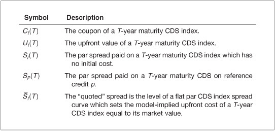
Because the quoted spread convention assumes that the spread curve is flat, there is a one-to-one mapping (based on the pricing model that we will describe below) between the T-year maturity quoted flat CDS spread and the upfront cost of a T-year CDS contract. Note also that if the par spread curve is actually flat, then the quoted flat spreads will all be the same for all maturity points and par and quoted flat spreads will be equal.⁴ In order to assist clarity, we will be using the notation in Exhibit 67–3 to denote these different coupons and spread measures in what follows.

EXHIBIT 67–3
Notation for Spreads and Coupons

MODEL

To value a CDS, we need a model. This model must satisfy the following requirements:

1. It must capture a credit event as a single event that can occur at any future time.

2. It must capture the timing of the default and the fact that the market may expect the future default rate to be a varying function of time, i.e., it can have a term structure.

3. It must capture the payment of par minus the recovery rate following a credit event.

4. It must be able to reprice the term structure of market prices exactly.

5. It must be fast to calibrate to the market and fast to price.

The standard model in the market is based on the use of the survival probability Q(T). This is the probability that the reference credit survives without experiencing a credit event from today (time zero) to time T in the future. The value of Q(T) must be between 0 and 1, and must be a constant or decreasing function of T.

Valuation of the Premium Leg

The premium leg of a CDS is the payment of the fixed coupon that continues at quarterly intervals until a credit event or maturity, whichever occurs first. Each coupon is therefore a conditional payment—conditional on the reference entity surviving until the coupon payment date. We also need to discount these future conditional coupons at the LIBOR rate. If we assume that the premium leg has N remaining coupons, we can write

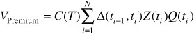
That is, for each payment date we multiply the fixed coupon C(T) by the year fraction Δ(t_i−1, t_i) since the previous coupon payment date in the corresponding basis.⁵ We then weight it by the probability of the reference entity surviving to the coupon payment date by multiplying by Q(t_i). We finally discount it back to today at the LIBOR rate using the discount factor Z(t_i).

By itself, this equation fails to take into account the coupon accrued that has to be paid if there is a credit event between coupon payment dates as it assumes that the CDS only pays a coupon if the reference credit survives up to the coupon payment date. An exact calculation of the value of the contribution of the coupon accrued is beyond the scope of this chapter. However, we can approximate the value of the contribution by simply assuming that if the reference credit experiences a credit event in the period before the coupon is paid, it will on average occur in the middle of the period. In this case, the amount of accrued coupon will be

i.e., one half of the full coupon. The probability of defaulting in the period before the coupon is due to be paid is given by Q(t_i−1) - Q(t_i). For simplicity and without any significant loss of accuracy we can assume that this is then paid at the end of the period. We therefore have a coupon accrued contribution given by

Adding this to the value of the premium leg above gives

We can rewrite this as

V_Premium = C(T) A(T)

where

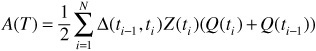
The quantity is known as the risky annuity. It is the expected present value of the premium leg assuming it pays an annualized coupon of $1 and any accrued fraction of this coupon if there is a credit event. It is a function of the entire shape of the survival curve since each premium payment is weighted by the survival probability to the premium payment date.

Value of the Protection Leg

The protection leg pays (1 − R) at the time of a credit event.⁶ To find the present value of this we have to take into account when the payment occurs. We need to split the time between today and the end of the contract into lots of small intervals and determine the probability of defaulting in each small time period and then discount the payment back to today.

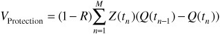
Suppose we split the time between now, time 0, and the maturity date in T years into M such intervals of length T/M. The value of the protection is then given by

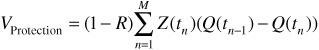
where (1−R) is the amount paid following a credit event, which we assume does not depend on the timing of the credit event, and Q(t_n−1) − Q (t_n) is the probability of defaulting between time t_n−1 and t_n.

In practice, the value of M must be a large number in order to best capture the full shape of the survival probability curve and the discount curve. However, it cannot be too large otherwise it would become numerically slow to price a CDS contract.⁷

The Upfront Cost

Here we define the upfront cost as the cost which must be paid by a protection buyer to enter into a CDS contract. It is therefore the expected present value of the protection leg minus the expected present value of the premium leg; that is, it is given by

U(0) = V_Protection − V_Premium

where

and

These are all at time 0.

The Upfront and the Par CDS Spread

The T-year par spread S(T) is the value of the coupon on the T-year CDS, which makes the current value of the contract equal to zero. Therefore

S(T)A(T) − V_Protection = 0 ⇒ V_Protection = S(T)A(T)

But the value of the contract at time zero using its actual coupon is

U(0) = V_Protection − C(T)A(T)

and we can substitute in the protection leg value to write this as

U(0) = (S(T) − C(T))A(T)

The situation changes when we calculate the value of the contract using the flat spread. This is simply defined via the equation

U(0) = ( (T) − C(T))(T)

This equation looks almost identical to the par spread valuation above. However there is one major difference. The value of the risky annuity here is only a function of the quoted flat spread (T), whereas the value of the risky annuity using the par spread is a function of the term structure of par spreads. Clearly, the quoted flat spread does not take into account the term structure of spreads.

Interpolation of the Survival Curve

Before we can use this model, we must calibrate it to the term structure of market prices. This can mean a number of things. It could mean calibrating it to a term structure of upfront costs, a term structure of par spreads, or a term structure of flat spreads. Whichever it is, we will usually have market price data at maturity points starting at six months and then up to 10 years in annual steps. To use these 11 market prices to calibrate a term structure of survival probabilities we need to simplify the term structure of survival probabilities so that it is described by exactly 11 variables. Then we will have one unknown variable for each piece of data and we should then be able to fit exactly the market prices using this simplified term structure.

There are many ways to do this simplification. The market standard is to introduce the continuously compounded forward default rate h(t). This is defined in terms of the survival probability as

A common simplification is to assume that this continuously compounded forward default rate is piecewise flat as shown in Exhibit 67–4.

Given 11 market prices, the term structure of this continuously compounded forward default rate takes 11 different values: h(0.5), h(1.0), h(2.0), . . . , h(10), where each h(t) is the value of the continuously compounded forward default rate from the previous time to time t. We then have

Q(0.5) = exp(−0.5 × h(0.5))
Q(1) = Q(0.5) × exp(−0.20 × h(1.0))
...
Q(10) = Q(9.0) × exp(−h(10.0))

EXHIBIT 67–4
Piecewise Flat Term Structure of the Forward Default Rate in Which We Calibrate to the 6M, 1Y, 2Y, ..., 10Y CDS Upfront Prices

However, the power of this approach is that it allows us to interpolate the value of the survival curve to other times. So for example we have

Q(0.3) = exp(−0.3 × h(0.5))
Q(0.7) = Q(0.5) × exp(−0.20 × h(1.0))
Q(1.9) = Q(1.0) × exp(−0.90 × h(2.0))

The whole term structure of survival probabilities is determined by these 11 values of the continuously compounded forward default rate. As long as the value of h(t) is greater than or equal to zero, the term structure of CDS spreads will be arbitrage-free.⁸

Calibration by Bootstrap

Given the model and this interpolation scheme, we need one more input before we can calibrate the values of the continuously compounded forward rates to the market prices of CDS. This is the value of the expected recovery rate R. Note that this does not have to be the same value as the one used by the market to convert the flat quoted spread to an upfront and back which is currently set equal to 40%. It can be a value chosen by the model user.⁹ With all of this information, the calibration can then be performed. This is done using a bootstrap.¹⁰ The process is as follows:

1. Search for the value of h(0.5) for which the model-implied upfront value equals the market quoted upfront of the six-month contract given the fixed coupon. As there is one unknown and one price, we should be able to determine h(0.5) so that the market price is fitted exactly.

2. Using h(0.5), now search for the value of h(1.0) for which the model implied upfront equals the market quoted upfront of the one-year contract given its fixed coupon.

3. Repeat step two for each next longer maturity CDS, each time using knowledge of all the previously calibrated values of h(t) to calculate the next one.

At the end of this process, we should have a value of h for each market price. From this we are able to compute the market-implied value of Q(T) to any future time T. The value of Q(T) that emerges from our market calibration is the “risk-neutral” survival probability. By risk-neutral, we mean the probability that, according to our model, reprices the market prices of CDS spreads—any other set of probabilities would not reprice the market and hence could create arbitrage possibilities. These spreads are credit-specific, forward-looking measures of the compensation required by a protection seller to sell protection until time T.

It is generally found¹¹ that credit spreads overcompensate the investor for the expected loss based on the incidence of default of other credits that had the same credit rating. There are a number of reasons why this may be the case. Mainly it is because the market is forward looking and may not consider historical default probabilities, especially when averaged over an economic cycle, to be appropriate given the current state of the economy. Also, because there is typically a large systemic and hence nondiversifiable component to credit spreads, investors demand an additional premium.

NEW AND EXISTING CONTRACTS

The price calculated by a CDS valuation model is the full price, i.e., the cash amount actually paid for the protection. One of the contractual details which determines this value is the date when the contract starts accruing the premium. In order to improve market fungibility of CDS contracts, the standard is for all new contracts to have a full first coupon; i.e., they begin accruing from the previous coupon payment date even if the contract was traded and settled more recently. This makes all contracts with the same maturity date identical in term of their cash flows. It also means that a hedger who buys protection mid-payment period will have to pay for protection that was not received and should expect to be reimbursed for this through the value of the upfront payment. After all, the upfront cash amount to be paid to enter into this contract for protection is the expected present value of the protection leg minus the expected value of the premium leg. This premium leg will include a full first coupon.

The simplest example we can use to examine the effect of this is to assume that the CDS has a fixed coupon of 100 bp and the par spread to the same maturity is also at 100 bp. However, the par spread is based on a CDS contract which starts accruing at T + 1, i.e., one day after the trade date, which must by definition have zero upfront value. Calibration of our CDS model determines the survival probability curve that ensures that this is the case. In more general terms, the value of the same maturity CDS used to calibrate the CDS valuation model is given by:

U_Calibration(t) = V_Protection −C(T)A(t,T) = 0

If we then use this curve to price our existing contract, we will find that the value of the contract will be

U_Contract (t) = V_Protection − C(T)A(t₀,0)

where t₀ is the time of the previous coupon. But we can then write

A(t₀,T) ≈ A(t,T) + Δ(t₀, 0)

which should be a very good approximation.¹² This gives

U_Contract (t) = VProtection − C(T)A(t,T) − C(T)Δ(t₀, 0)

The first two terms on the right-hand side equal the value of the CDS contract we are calibrating to which is zero, and so we have

U _Contract (t) = −C(T)Δ(t₀,0)

This is the negative of the coupon which has accrued since the previous coupon date. The protection buyer therefore finds that the contract pays him for the portion of coupon which accrued since the last coupon date which he has to pay on the next payment date, but whose benefit he did not enjoy since he wishes to enter the contract today. Clearly the payment of the coupon can be up to three months in the future (this is offset by the fact that the further in the future the coupon payment occurs the less that has accrued) while the upfront cost is paid on the settlement date which is trade date plus three days, holiday adjusted. For this reason, setting the value of the contract equal to the negative of the accrued coupon is a good approximation but one that would only be exact in a world of zero interest rates.

There is one more issue to consider—the CDS contract provides protection against a credit event which occurred between T-60 and today. If such an event has been determined by the Determinations Committee (see Chapter 66) then the CDS contract would be in its post-credit event settlement process and the upfront cost would be close to par minus the expected recovery rate. If the event has not been determined, the implicit assumption is that market expectations that a credit event occurred in the past 60 days are already priced into the CDS spread curve.

RISK MANAGEMENT

We now wish to understand the factors that drive the valuation of a CDS contract. Specifically, we want to be able to calculate the hedge ratios needed to ensure that the value of a portfolio of CDS contracts on the same reference credit is immunized against parallel moves in the CDS spread curve and the LIBOR interest rate curve. We begin by writing the time t upfront value of a (short protection) CDS contract as

U(t,S(t,T)) = (C −S(t,T))A(T,(T,S(t,T))

where S (t, T)is the time T maturity par CDS spread as seen at time t. Note that we have inserted an explicit par spread dependency into the upfront value and the risky annuity term A (T, S (t, T)) to remind ourselves that a change in the par spread followed by a recalibration will cause the term structure of survival probabilities to change and so will change the present value of the risky annuity and the value of the upfront.

Spread DV01 of a CDS

The credit duration of a CDS contract is usually known as the Spread DV01. It is defined as the change in the upfront value of the contract for a 1 bp parallel bump upwards in the CDS spread curve. For a short protection position, we can write this as

Spread DV01 = U(t,S + 1bp) − U(t,S)

This gives

Spread DV01 = −A(T,S + 1bp + (S − C).(A(T,S)−A(T,S+1bp))

There are two contributions to the Spread DV01:

1. The first term describes a fall in the upfront value of the short protection position by A(T, S 1 bp) times the change in the spread. The value falls because we have sold protection and the credit quality of the reference credit, as implied by the spread which was bumped, has worsened so the position has lost value.

2. There is a second term due the fact that the change in spread also causes the value of A(T, S) to change. Because this term is multiplied by the spread difference (S − C), it is usually much smaller then the first term. Also, the sign of the change is driven by the sign of (S − C). If this is positive, it means that this term will offset the effect of the first term and reduce the Spread DV01. If negative it can increase the Spread DV01.

The Spread DV01 of a short protection position is therefore typically close in value to the negative of the risky annuity given by A(T, S) multiplied by 1 basis point and approaches¹³ it if S = C. The spread sensitivity from the perspective of a long protection position is simply the negative of that of a short protection position.

Hedging different CDS positions using the Spread DV01 is only really effective if the quoted spread or par spread of the different contracts move by the same amount. For contracts of differing maturity, this requires the CDS curve to move in parallel shifts, which is not always the case. For this reason, use of the Spread DV01 should generally only apply to contracts of a similar maturity. To go beyond Spread DV01, we would need to calculate the sensitivity of a CDS contract to movements of different curve points (e.g., one year, three year, five year, seven year, and 10 year), and determine the set of positions in each of these contracts needed to immunize the hedged portfolio against spread movements.¹⁴

Interest Rate Duration of a CDS

The interest rate sensitivity of a CDS contract is known as its IR DV01. It is defined as the change in the upfront value of the contract for a 1 bp parallel bump upwards in the LIBOR curve while keeping the par spread curve fixed. As the only interest rate dependency is in the annuity term, we have

IR 01 = (C − S). (A*(T) −A(T))

where A*(T) is the value of the risky annuity calculated using the bumped interest rate curve. Since this is the present value of future cash flows, we can conclude that A*(T)−A(T) < 0. We can therefore conclude that: (1) if C = S the interest rate sensitivity of a CDS is zero, (2) if S > C then the IR DV01 is negative, and (3) if S < C then the IR DV01 is positive.

In general the interest rate sensitivity of a CDS is low, especially when compared with a fixed-rate corporate bond with the same maturity date. This is due to the fact that the bond has coupons plus a payment of par at maturity, while the CDS is effectively a credit risky annuity with annualized coupon payments of (C − S) and unlike a bond there is no payment of par at maturity. In fact the interest rate sensitivity of a CDS actually close resembles the interest rate sensitivity of a same-maturity par floating rate note issued by the reference entity.

Example

Exhibit 67–5 shows an example¹⁵ of the pricing of a real CDS trade to buy protection until March 20, 2016. The CDS coupon (deal spread) has been fixed at 100 bp. The pricing of the CDS is captured by the current flat spread, called the “quoted spread,” to the contract maturity date, which is 34.32 bp. This is the only spread quote needed to determine the upfront value. Both the deal and the quoted spread assume the market standard recovery rate of 40%.¹⁶

EXHIBIT 67–5
The Value of the CDS Contract

We explain the valuation outputs in Exhibit 67–5:

• Price: This is the “clean” price for a protection seller who was to buy the CDS together with a par LIBOR floating rate note. It excludes the payment of accrued interest that would need to be added to the actual price paid.

• Principal: This is the clean (excluding accrued interest) value of the contract. It is computed by subtracting the accrued interest from the cash amount defined below.

• Accrued Interest: This is the amount of coupon that has accrued since the last coupon payment date or the first accrual date. For a new contract and an existing contract this is always the CDS Date that falls before the trade date. For a protection buyer the accrued interest is always negative while for a protection seller it is always positive. The valuation shows 46 days of a 100 bp coupon that has accrued from the previous payment date on 20 December 20, 2010 to T+1 calendar, which falls on February 4, 2011.

• Cash Amount: This is the actual upfront amount that has to be paid to enter into this contract. The valuation is –$334,813 meaning that the protection buyer receives $334,813 to enter into this contract. This is because the protection buyer who enters into this contract has to pay an annualized coupon of 100 bp for up to five years for a reference entity with a quoted flat spread of 34.32 bp. Because the coupon being paid is higher than the cost of protection implied by the quoted spread, the protection buyer has to be compensated upfront.

• Spread DV01: The spread sensitivity of the long protection position is calculated to be $5,036, meaning that a 1 bp increase in the quoted spread curve would cause the value of the CDS position to increase by this amount.

• IR DV01: The interest rate sensitivity of the contract is also positive, but much smaller at $84.24. This makes it very clear that a CDS is almost purely a credit-spread product.

Exhibit 67–6 shows the cash flows on the premium leg of the CDS. We see the payment dates and the corresponding amounts calculated using the Actual 360 day count convention. We also see the discount factors implied by the LIBOR deposit rates and swap rates used. Finally we see the survival probabilities implied by our CDS valuation model. The default probability is simply one minus the survival probability.

EXHIBIT 67–6
Payment Dates, Amounts and the Corresponding Discount Factors and Survival Probabilities for the Example CDS Trade. Note that the Payment Dates Have Been Holiday Adjusted.

Approximation

For those wishing to evaluate trading strategies, the Bloomberg pricer found under CDSW can be limiting and a simple Excel-based pricer would be quite useful, even if it is not exact. It is therefore worth describing a simple approximation that is based on the observation that the value of the risky annuity of a new CDS contract can be linked directly to the quoted flat spread and the recovery rate assumption R using the following approximation

where W is the swap rate to the contract maturity in T years and the ratio of 365/360 is used to adjust for the Actual 360 convention used to determine the size of premium payments.¹⁷ The value of a long protection CDS position is simply given using the standard valuation equation:

Taking the example above where the quoted spread is 34.23 bp, the time from today to contract maturity is 5.122 years and the 5-year swap rate is 2.4%, we find that

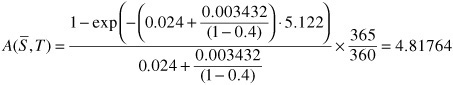
We therefore calculate

This should be compared to the cash amount calculated by the Bloomberg valuation (not shown) which was −$334,813, a difference of about $5,000 on a $10 million face value. Note that we had to subtract the 46 days of accrued coupon which have to be paid by the protection buyer at the end of this coupon period. These are worth $12,778. The reason for doing this is that this contract requires the protection buyer to pay a full coupon on the next payment date. However the quoted spread of 34.32 bp is for a contract that starts accruing from T + 1. To account for this we need to compensate the protection buyer for having to make this extra future payment and to a very good first approximation, this can be done by subtracting the accrued coupon. The valuation is within 1.5% of the Bloomberg result—corrections to the interest rate used to discount the CDS cash flows to account for the slope in the swap curve can further improve the accuracy of this approximation.¹⁸

CDS INDEX VALUATION

The mechanics of the CDS index have been set out in Chapter 66. We showed that a CDS index is equivalent to a portfolio of CDS in which the individual CDS all pay the same index coupon given by C_I(T). In this section, we wish to show that for valuation purposes a CDS index can actually be treated as though it were a CDS contract. We recall from Chapter 66 that the buyer of a time T-maturity CDS index is selling protection on a portfolio of P different time T-maturity CDS contracts, and receiving a coupon C_I(T) in return for assuming this risk. Credit events in the portfolio result in the relevant CDS being removed from the index and settled via the standard auction procedure described in Chapter 66.

On each coupon payment date the size of the coupon payment is proportional to the size of the remaining portfolio of CDS. It therefore falls in absolute terms as credit events occur.

Therefore, unlike a single-name CDS, a CDS index does not have a single credit event which causes it to pay out a single loss and then cancel. Instead, the contract remains active¹⁹ until maturity, with loss payments being made as and when credit events occur.

Index Valuation

From the perspective of an index buyer (protection seller), the CDS index value is equal to the premium legs of the P underlying CDS contracts that each pay the index coupon, minus the expected present value of the P protection legs. Using the notation set out in Exhibit 67–5, we can therefore write the value of the index premium leg as

EXHIBIT 67–7
Notation Used in the Valuation of CDS Indices

We can also write the value of the index protection leg in terms of the individual CDS spreads as

We are assuming here that the reference credits are all equally weighted.²⁰ The value of the index (short protection) position is then

The most common application for CDS index pricing is Bloomberg’s CDSW function. This treats a CDS index as a standard CDS contract. As with CDS, price quotations for the CDS indices are almost exclusively done using the “quoted” flat index spread defined as the level at which we would mark a flat CDS index par spread so that, when using the standard CDS pricing model, it would cause the index model price to refit the market upfront index price. We therefore have

The point here is that this mapping of a CDS index onto a single CDS contract allows us to use our single-name CDS analytics to value and risk manage the CDS index. By doing so, we price the CDS index as though it has its own index survival probability Q_I(t). Note that if we assume that the expected recovery rates of all of the credits in the index are the same, we can write

where N_I(t) is the expected surviving notional of the index at time t. We do not use this relationship in pricing because it assumes that all recovery rates are the same, which is not always the case. However, in general, it is approximately true and does provide some intuition about the interpretation of the index survival probability.

The CDS Index Basis

If this relationship is not obeyed, there is then a theoretical mispricing. However, this theoretical mispricing may not be arbitrageable for a number of reasons:

1. Model prices are usually mid-market. Therefore, if we take into account the cost of crossing the bid-offer spread that would need to be done to monetize any mispricing, this mispricing may not be a real arbitrage opportunity after all.

2. Obtaining accurate and contemporaneous flat spreads for all of the constituents of a CDS index may not be possible.

3. Where CDS and CDS indices trade with different restructuring clauses, the replication is not exact and this relationship should not be exactly obeyed.

Despite these caveats, CDS indices have traded away from their CDS-implied spread. This will generally be due to market technical factors such as a market demand to buy or sell systemic versus single-name credit protection. If the deviation becomes large enough to be arbitraged, then hedge funds and other market players will step in to monetize the profit until their activities eliminate the arbitrage.

Risk Management

Since the CDS index contract is valued as though it was a single-name CDS contract, its price sensitivities are identical to those of a single-name CDS contract with the same term structure of par spreads or quoted spread, the same recovery rate, the same maturity and the same interest rate environment. As a result, we refer the reader to the section on CDS risk management.

KEY POINTS

• Since the introduction of fixed coupons for CDS contracts in 2009, entry to a CDS contract almost always involves some initial upfront cash payment, which can be positive or negative.

• From the perspective of a protection seller, the size and sign of the initial cash value of the contract depends on whether the fixed coupon is sufficient to compensate the protection seller for the market perceived risk of a credit event. If the coupon is low, the protection seller may receive cash at trade initiation. If the coupon is high, the protection seller may have to pay cash at trade initiation. The situation is reversed for a protection buyer.

• The purpose of the valuation of CDS and CDS indices is to calculate this upfront cash payment. This requires a model in order to determine the expected present value of the premium and protection leg of the contract.

• This model needs to take into account the probability of and the timing of a credit event. For the premium leg, it needs to take into account the risk that not all coupons will be paid. For the protection leg it needs to value the unknown payment of par minus recovery made at the time of the credit event, if one occurs. It also needs to be flexible enough to exactly reprice the term structure of quoted market spreads.

• One type of market quote is the CDS par spread. This is the value of the coupon that would need to be paid on the premium leg of a CDS in order for the contract to have zero upfront value on trade date. The value of a CDS is a function of the term structure of CDS par spreads.

• Since 2011, the CDS market has also begun to use an alternative measure known as the flat “quoted” spread. This is the level at which a flat term structure of par spreads would need to be set in order that they reprice the market quoted upfront value. As a result, only one quoted spread is needed to value a CDS contract.

• The probability of a CDS experiencing a credit event as implied by CDS market spreads usually exceeds the historical default probability implied by the default rate of credits that were initially assigned the same credit rating. This is because spreads are forward-looking and embed a risk premium.

• The model allows the holder of a CDS position to calculate the sensitivity of the value of the contract to changes in the quoted spread and so enables him to hedge it with other CDS contracts.

• For valuation purposes, a CDS index can be treated as a single-name CDS and valued and risk-managed using the same model as the CDS.