
CHAPTER
SIXTY-NINE
PRINCIPLES OF PERFORMANCE ATTRIBUTION
Managing Director
Barclays Capital
ANTÓNIO BALDAQUE DA SILVA, PH.D.
Director
Barclays Capital
CHRIS STURHAHN
Vice President
Barclays Capital
ERIC P. WILSON
Vice President
Barclays Capital
PAM ZHONG, CFA
Vice President
Barclays Capital
Performance measurement and attribution is an important function of portfolio management. It helps bring clarity to the sources of portfolio risk and performance, quantify the contributions of individual decision-makers and identify structural issues. Performance attribution algorithms typically follow either a sector-based allocation or a factor-based allocation methodology, but neither is sufficient to cope with the complexity of modern portfolio management. In this chapter, we first discuss the principles of performance attribution. We review the sector-based and factor-based attribution frameworks then describe a hybrid attribution model1 that blends the two and has the flexibility to adapt to the particular management structure of most portfolios. The chapter finishes with the application of performance attribution, both as a portfolio management tool and a data quality tool. Where possible, we introduce the best practices for performance measurement and discuss practical considerations in real-world applications. Throughout the chapter, we utilize examples produced by the Barclays Capital Hybrid Performance Attribution (HPA) model2 as implemented in POINT, the Barclays Capital portfolio analytics and modeling platform.3
PRINCIPLES OF PERFORMANCE ATTRIBUTION
Managing a global diversified portfolio of financial assets is a complex task that requires adopting views in different markets and implementing them with regular trading activities. Expressing and implementing views in a variety of markets that interact with each other in complex ways, makes it very difficult to quantify the contribution of each decision-maker to the performance of the portfolio. Performance attribution is a mathematical framework that attempts to split the total outperformance of a portfolio versus a benchmark into the contributions of individual decisions and actions.
Complex portfolios are typically managed by breaking down the investment process into a sequence of decisions made by different managers, each of whom specializes in a specific market or type of security. Traditionally, this process follows product and sector lines. Risk-factor-based portfolio management became popular with the advent of modern portfolio risk management and the realization that certain risks are common for multiple asset classes. Foreign exchange (FX) and interest rates are examples of risks that are now commonly being managed separately for the entire portfolio while product/sector experts focus on managing excess returns.
The total outperformance of a portfolio depends on the combined outcome of the decisions of all portfolio agents, as well as the market performance. Often, the effects of different agents’ decisions depend on each other in a way that makes it difficult to disentangle them. A successful performance attribution algorithm will do so in a way that satisfies three important requirements:
• Additivity: The contribution of two or more agents combined is equal to the sum of the contributions from those agents.
• Completeness: The sum of all outperformance contributions is equal to the total portfolio outperformance.
• Fairness: The allocation of outperformance to different interacting agents is performed in a way that is perceived to be fair by all agents.
These requirements are important because performance attribution is often used to measure the skill level and determine the compensation of portfolio managers. The fair decomposition of portfolio outperformance must take into account the management structure of the portfolio. In addition, a good performance attribution model or system needs to successfully address multi-period compounding and have sufficient flexibility in order to meet the demands of modern portfolio management.
Multi-Period Attribution and Compounding
Generally speaking, a performance attribution model measures the exposure of a portfolio to various markets at the beginning of a period and then explains the contribution of each market to the performance of the portfolio over the period as the product of its exposure to the market times the market move. Since actively managed portfolios dynamically adjust exposures to various markets frequently, such performance attribution over a period of time will not capture the effect of active portfolio management.
For example, consider a portfolio that begins the attribution period with no exposure to a particular sector. During the period the sector rallied and in response the manager allocated positive exposure to the sector. Subsequently the sector lost all of its gains and ended the period flat. Since the portfolio had no exposure when the sector rallied but positive exposure when the sector retreated, the portfolio realizes losses over the period. An attribution system that looks at exposure at the beginning of the period (zero) and the return of the sector over the period (also zero) will not be able to explain the realized losses. A system using average exposure over the period will also fail to explain the losses since the return of the sector is zero over the period. On the other hand, a system that splits the attribution exercise in two (or more) subperiods and then combines the results of the subperiods to explain the total portfolio performance over the entire period will be able to identify the intra period exposure adjustment as the reason for the portfolio losses.
The length of the subperiods that an attribution system uses to explain performance over longer periods determines the frequency of the attribution system. Linking the returns of subperiods is called compounding. Timing affects investment performance, especially when intermediate cash flows occur. Since cash flows impact portfolio market value, the fundamental question is whether sub-period returns should be compounded without regard to the portfolio size during each subperiod (time-weighted compounding) or whether subperiod returns should be weighted by the portfolio market value in each period (money-weighted compounding). For example, consider a portfolio with a seed investment of $1,000,000 that earns a rate of return of 100% doubling its value for the first half of the year. Because of its success, the portfolio attracts additional investments of $100,000,000 and its market value becomes $102,000,000. Unfortunately, in the second half of the year it has losses of 10% ending the year with a value of $91,800,000. What is the annual return of the portfolio? Assuming the inflow occurred in the middle of the year, money-weighted rate of return estimates the annual return by solving for the internal rate of return:
1,000,000 × (1 + r) + 100,000,000 × (1 + r)0.5 = 91,800,000 ⇒ r = −17.24%
Time-weighted rate of return ignores the portfolio size and reports an annual return of:
r = (1 + 100%) × (1 −10%) −1 = 80%
Given the dramatic differences between the two methods when portfolio flows are significant relative to its current size, the choice between the two methods is an important decision. Whether the timing of cash flows should be reflected in return measures depends on whether the portfolio manager is responsible for the timing of the cash flows. If she is responsible, then money-weighted method should be used. In the case of mutual fund or pension fund managers who have no direct control of cash contributions and withdrawals, the time-weighted method is more appropriate. In the following three chapters we assume the time-weighted methodology.
Once the method for compounding returns is decided, the question of splitting multi-period returns into components (i.e., multi-period performance attribution) must be addressed. The difficulty arises from the fact that compounding is a nonlinear function and introduces interaction terms that must be allocated between different return components. For example, consider that the portfolio return is attributable to two components which both contribute 10% of return over two periods. The return of the first component is realized during the first period, and the return of the second component is realized over the second period. Time-weighted compounding will report total portfolio return of (1+10%) × (1+10%) – 1 = 21%. Each component contributes 10%, leaving 1% of total return that can be claimed by either component. A multi-period attribution system must adopt both return and outperformance compounding algorithms that retain the principles of additivity, completeness and fairness. Such algorithms are discussed in more detail in Chapter 71.
It is important that the frequency of the attribution system match the frequency of portfolio management decisions. If the attribution frequency is too low, as in the example above, part of the portfolio performance may remain unexplained. Conversely, if the attribution frequency is too high, the attribution model may attribute outperformance to portfolio management erroneously. Many fixed income portfolios are managed on a daily basis, especially with respect to their interest-rate exposures; therefore daily-frequency attribution models are commonly used for fixed income portfolios. Daily compounding generates the requirement for high-quality daily prices and analytics for all securities in a portfolio and its benchmark. Sophisticated attribution systems can be used as a magnifying glass for data quality. Any problems with the data are immediately shown in the quality of the results. An example of this is discussed later in the chapter.
Flexibility
A practical performance attribution system must reflect the decisions that a portfolio manager makes during the normal course of the investment process. With a wide diversity among portfolio managers also comes a wide diversity of styles that are often mutually exclusive. No single specification of a performance attribution can describe all managers’ preferences. In order to be useful, the model must also satisfy the following requirements:
• Measure the risk factors corresponding to the portfolio managers’ decisions
• Independently measure the contributions of each factor in the portfolio management process
• Closely follow the published returns of the fund, and its benchmark
• Be available in a timely manner
• Have sufficient adaptability to explain both short and long time periods
In short, it must be useful to the portfolio manager in explaining and refining her decisions, quantifying the effects of the investment process.
MATHEMATICS OF PERFORMANCE ATTRIBUTION
Performance attribution algorithms typically follow either a sector-based allocation or a factor-based allocation methodology. Both methods follow the same framework which expresses the total outperformance of the portfolio over a benchmark RP − RB as the sum of several components. The contribution of each component is determined by a portfolio manager’s decision to allocate a different exposure than the benchmark to a particular market or factor, and the performance of the market or the factor itself. In this section, we first discuss sector-based and factor-based attribution under this simple framework, and then introduce a hybrid model that blends the two and has the flexibility to support virtually all types of portfolios and portfolio management styles. We will develop the mathematical framework of performance attribution assuming a generic set of sectors and factors. In Chapters 70 and 71 we will see the application of this framework in the performance attribution of fixed income portfolios.
Sector-Based Attribution
In its simplest form, portfolio management versus a benchmark is modeled as a two-step process that consists of market weight allocation to various sectors and security selection within each sector. The classical performance attribution methodology is often referred as “Brinson model.”4 Portfolio return is the market value-weighted (ws) sum of the individual sector returns, Rs:
![]()
Similarly, benchmark return is the weighted sum of benchmark sector returns:
![]()
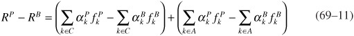
This representation allows us to identify two key drivers of the total outperformance RP − RB: the differences in the sector allocations, ws, a and the differences in the returns, Rs earned within each sector. The outperformance achieved by reweighting the sectors is called “Asset Allocation,” and the outperformance due to the intrasector return differences is called “Security Selection.” To make the decomposition of the total outperformance complete, we need to add a third term, the “Interaction” effect, the joint effect of asset allocation and security selection.
![]()
![]()
![]()
Interaction terms arise every time two factors contribute to outperformance through a non-additive function such as the product. Interaction terms are philosophically undesirable, since the stated goal of performance attribution is to credit agents separately for their contribution. Thus, we attempt to merge interaction terms into other outperformance components that can be uniquely attributed to a single agent. The criteria for consolidation are usually dictated by the order in which decisions are made, or the relative size of the interaction term.
The standard assumption is that asset allocation precedes security selection (i.e., the portfolio is managed in a top-down fashion), so it is common to fold the interaction term into the latter:
![]()
![]()
If, on the other hand, the expected returns of sectors in the portfolio are different than those in the benchmark (for example, because of manager skill or leverage), then it might be more appropriate to fold the interaction term into asset allocation instead. As a result, asset allocation would be given by ![]() and security selection would be given by
and security selection would be given by ![]() . It is easy to see that in both cases, the outperformance breakdown is complete; i.e., the sum of the two components is equal to the total outperformance.
. It is easy to see that in both cases, the outperformance breakdown is complete; i.e., the sum of the two components is equal to the total outperformance.
The above formulas would assign positive contribution to asset allocation outperformance to any overweighted sector with positive benchmark sector return. Thus, if all sectors have positive benchmark returns, overweighting the sector with the worst return would still be considered a good decision. This is intuitively wrong in most portfolios, as the weight allocated to such sector would be better used in sectors with higher returns. Therefore, instead of using the absolute benchmark sector return in the above asset allocation formula, one can use the sector return relative to the benchmark return (which represents the weighted average return of all benchmark sectors):
![]()
![]()
Notice that while the contribution of each sector to asset allocation changes, the total asset allocation outperformance remains the same as long as ![]()
The constraint that the sum of the portfolio and the benchmark sector weights are equal to one necessitates the comparison of the benchmark sector returns with the overall benchmark return. If leveraging is allowed, such that there is no constraint on each sector’s weight, then each overweighted sector with a positive return should indeed have a positive contribution to outperformance. In such a case, we do not need to compare the return of each sector to the return of the benchmark and Eqs. (69–4) and (69–5) apply. In practice, however, leverage constraints do exist (usually dictated by risk constraints), and neither the benchmark return nor zero is a generally appropriate choice for the hurdle rate for each sector. In the following discussion, we will use the term RH generically for the hurdle rate. This formulation describes both above models while allowing for extra flexibility. A choice of RH = 0 gives the original Brinson model in Eqs. (69–4) and (69–5), while a choice of RH = RB gives the model in Eqs. (69–6) and (69–7).
Recursive Allocation
Most large portfolios have many management layers by which allocation decisions are made successively. For example, the global strategist can specify the allocation into global markets, the U.S. strategist can determine the allocation to major asset classes in the U.S. (equities, bonds, commodities, etc.), the fixed income strategist can determine the allocations into the various sectors, and so forth.
In such a case, what we called security selection above contains not only security selection, but also further asset allocation, as well as security selection for each subsector. In fact, each sector can be considered as a smaller portfolio for which the above performance breakdown equations can be applied recursively. For this reason we will use the term “Sector Management” instead of “Security Selection,” and we will reserve the term “Security Selection” for the last layer of management when no further sector decomposition occurs.
For each sector, its contribution to the sector management from the level above, ![]() , is recursively split into the following components:
, is recursively split into the following components:
![]()
![]()
Typically, the benchmark sector return ![]() is used as the hurdle rate as for the calculation of asset allocation to subsectors. In this fashion, we can keep decomposing sector management outperformance until we reach the last layer of portfolio management. Since at each level the decomposition is complete, the total outperformance decomposition is also complete. This algorithm has two of the three required properties of performance attribution: additivity and completeness. As we will see in the following discussion, it also has sufficient flexibility to be applied under different management structures such that it is considered to be fair, thereby satisfying all three requirements of performance attribution.
is used as the hurdle rate as for the calculation of asset allocation to subsectors. In this fashion, we can keep decomposing sector management outperformance until we reach the last layer of portfolio management. Since at each level the decomposition is complete, the total outperformance decomposition is also complete. This algorithm has two of the three required properties of performance attribution: additivity and completeness. As we will see in the following discussion, it also has sufficient flexibility to be applied under different management structures such that it is considered to be fair, thereby satisfying all three requirements of performance attribution.
The fundamental advantage of the sector-based attribution methodology is its flexibility. The ability to analyze portfolio allocations along an arbitrarily specified market partition makes it possible to customize the model to fit many different types of portfolios and management styles. The main disadvantage of this approach is that it analyzes yield-curve and spread returns within the same market partition using market value weights, something that does not correspond to standard fixed income portfolio management practice.
Factor-Based Attribution
The “sector-based” attribution is gradually losing ground to a “factor-based” decomposition of the investment universe, where the return of the security in the portfolio/benchmark is decomposed into the contributions of common risk factors plus a residual. The residual represents the return not captured by the risk factors. The coefficients of the factors, αk, are called loadings or sensitivities of the portfolio to each factor, fk. Typically, the decomposition is linear and is represented as:
![]()
Such risk factors for fixed income securities include interest rates, implied volatility, spreads, etc., and the loadings are the corresponding sensitivities to the exposure of each factor (option-adjusted duration, partial (key-rate) durations, Vega, spread duration, and related measures). Factor-based attribution essentially entails the decomposition of outperformance to the contribution of each risk factor.
![]()
Pure factor-based attribution systems attempt to use a set of factors that can explain all of the systematic return of a portfolio. In this case the excess return is idiosyncratic and therefore quite small for a well diversified portfolio. The disadvantages of this approach are that it does not attribute idiosyncratic returns of small portfolios to security selection decisions, and there is usually little flexibility in defining the risk factors. The latter shortcoming may be overcome with factor remapping,5 which allows each portfolio manager to attain a personalized view of risk and return decomposition.
A Unified Framework for Performance Attribution
We will now combine the ideas we have developed in the preceding sections into a unified framework that blends the sector-based and the factor-based attribution. Models using this framework, such as the Barclays Capital Hybrid Performance Attribution model, are favored by portfolio managers since they can account for the complex management structures of large diversified portfolios. The framework offers enhanced flexibility in defining arbitrary hierarchical partitions along which sector allocation decisions are expressed. It allows the portfolio managers to achieve the best match to their investment decision-making process. It is a conceptually simple recursive algorithm that can be described in three steps: return splitting, factor return attribution, and recursive application. We explain these steps below.
Step 1: Return Splitting
The total return of the portfolio and the benchmark is split into the linear contributions of factors.6
![]()
Note that residual is included here as one of the factors with a loading of one.
Step 2: Factor Return Attribution
The factors from step 1 are categorized as either common or allocated. We denote the set of common factors by C and the set of allocated factors by A and write the total outperformance as:
The outperformance from each factor is then handled separately. For each factor, we partition the investment universe into sectors7 and decompose the outperformance from the factor.
![]()
Outperformance from common factors is explained using bottom-up aggregation, namely via net exposures to a factor at each level of the aggregation. Furthermore, if a factor is truly common, where the factor return in the portfolio is identical to the factor return in the benchmark, then the contribution of the factor to portfolio outperformance can be written as:
![]()
This breakdown allows the performance of the portfolio due to the common factors to be categorized and aggregated to the portfolio level. In this way, a more detailed explanation of the factor and its impact to the total portfolio is possible than if the return were split between sectors. For example, exposure to the yield-curve is typically managed at the portfolio level by determining first the overall duration over/underweight vs. the benchmark and then determining where on the yield-curve to take the extra exposure. The strategy may be designed to take advantage of flattening or steepening in the yield-curve, and only measurement of these effects at the portfolio or sub-portfolio level is meaningful.
Outperformance from allocated factors is explained using the following allocation methods: absolute allocation and relative allocation. We discuss each below.
Unlike common factors, allocated factors may have different realizations for different securities or sectors even if they broadly capture the same type of risk exposure. For example, credit-spread, whose level depends on the particular securities within a sector, is a factor of this type. In the absolute allocation framework, the total portfolio exposure to each factor is determined by all sector managers. Each sector manager may take a different view as to the expected direction of each factor. In this case, asset allocation is solely determined by the net sector exposure to a particular factor:
![]()
![]()
In the relative allocation framework, the total exposure to each factor is determined at the portfolio level (or the higher hierarchical level). The asset allocator subsequently determines the sector exposures to the factor subject to the constraint imposed by the portfolio exposure. Each sector may take a different view as to the relative movement of each factor against the overall benchmark factor return.

![]()
![]()
Notice that in the relative allocation framework, the factor hurdle rate ![]() essentially becomes a common factor.
essentially becomes a common factor.
Step 3: Recursive Application
The sector management terms from top-down allocations, ![]() , can be now decomposed separately using the above algorithm recursively.
, can be now decomposed separately using the above algorithm recursively.
At the last stage of the decomposition, in which a sector is not decomposed further into subsectors, the sector management term becomes security selection. The top-down decomposition can be applied one last time to break down the security selection outperformance of a sector into the contributions of individual securities. In this case the management term is typically zero, since the factor driving the return of the same security in the portfolio and the benchmark is the same.
An Example of Hybrid Performance Attribution
To illustrate how this algorithm can be applied in practice, consider a very simple model in which the return of a security is split into two components: the time return that is measured by the yield of the security and a market return that is measured as the duration of the security times the negative of its yield change. This decomposition may not be complete, so it is reasonable to assume the presence of a residual.
![]()
The portfolio (or benchmark) return is the weighted average return of the securities in the portfolio (or benchmark). The summation extends over a universe defined by the union of securities in the portfolio and benchmark. Securities not present in either get correspondingly zero weight.
Aggregation of yield and duration is the usual weighted average; however, yield changes must be aggregated using duration contribution weights to retain their natural interpretation.

![]()
We can now rewrite the portfolio and benchmark returns using top-level analytics:
Let us assume that time return (carry) and residual are allocated as common factors.
![]()
![]()
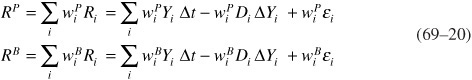
Market return is managed by allocating duration exposure ![]() to a set of sectors and allowing managers to pick securities within each sector.
to a set of sectors and allowing managers to pick securities within each sector.
If the top-level portfolio duration is not constrained and is completely determined by the choices of the sectors’ net duration exposures, we should use the absolute allocation algorithm by setting αk ← D, αk,s ← ws Ds, fk,s ← −ΔYs. The duration and yield change of each sector in the portfolio and the benchmark are calculated in the same weighted average fashion we discussed above. Since the asset allocation agent is free to determine the duration exposure of each sector, there is no hurdle rate and the total outperformance is solely distributed between asset allocation and security selection.
![]()
![]()
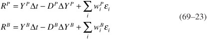
On the other hand, if the net duration of the portfolio is actively managed, we need to use the relative allocation method. In this case, we set the hurdle rate equal to the benchmark yield change.
![]()
![]()
APPLICATIONS OF PERFORMANCE ATTRIBUTION
Beyond its stated goal of attributing portfolio outperformance to the actions of agents, detailed and flexible performance attribution can bring clarity to the process of portfolio management by systematically exposing sources of risk and performance. By linking ex-post outperformance contributions to ex-ante views and management decisions, a manager can identify unanticipated sources of risk and return and adjust the management process accordingly. In addition, by providing the recursive decomposition of outperformance into the various contributing factors, it facilitates the discovery and correction of data errors that are not uncommon in large financial accounting systems. In the rest of this chapter we will illustrate such applications of performance attribution in the context of a particular portfolio.
Performance Attribution as a Portfolio Management Tool
Consider the following example. A portfolio manager has the mandate to track the Barclays Capital Global Aggregate G4 Index and has the latitude to implement certain market views in order to enhance the portfolio returns, as long as the standard deviation of portfolio minus benchmark returns (Tracking Error Volatility or TEV) stays below 40 bp per month. At a specific point in time, the manager is bullish on the Japanese yen, negative on the euro and neutral on the U.S. dollar and the British pound. She believes that global rates are falling. She has no sector views except in the U.S. markets, where she likes corporates but dislikes the securitized sector. According to her mandate and her views, she constructs a portfolio with the following characteristics:
• The portfolio has a 5% overweight (vs. the benchmark) in the yen, a 5% underweight in the euro and is flat in U.S. dollars and British pounds.
• The portfolio interest-rate option-adjusted duration (OAD) is about one year longer than that of the benchmark.
• Within the U.S. market, the portfolio has a 5% overweight in corporates, a 5% underweight in securitized, and is flat in the U.S. Treasury and government-related sectors.
We created this portfolio in the Barclays Capital POINT system and used the Global Risk Model in POINT to estimate the portfolio tracking error volatility relative to its benchmark as 32 bp per month. Since this is below the 40 bp per month risk budget the portfolio is acceptable.
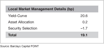
We subsequently ran the POINT hybrid performance attribution model over one month and produced a detailed performance attribution report. This report begins by reporting the total portfolio and benchmark returns over the month (+188.7 bp and +150.0 bp respectively) as well as their difference, +38.7 bp, the total portfolio outperformance (Exhibit 69–1). The report then proceeds to decompose the total outperformance into the contributions of the various portfolio exposures and market performance. The decomposition is hierarchical to allow the portfolio manager to first get a broad understanding of the sources of outperformance and then dive into the specific details. In Exhibit 69–2, we see a first decomposition of the portfolio total outperformance on a global level into three components: FX Allocation and Hedging (+28.3 bp), Local Market Allocation (–8.7 bp), and Local Market Management (+19.1 bp). In Exhibit 69–3, the Local Market Management component is further decomposed into contributions from Yield-Curve exposures (+20.6 bp), Asset Allocation (+0.2 bp) and Security Selection (–1.7 bp).
EXHIBIT 69–1
Total Portfolio Outperformance

EXHIBIT 69–2
Global Outperformance Summary
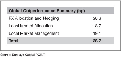
EXHIBIT 69–3
Local Market Management Details
Outperformance from Currency Exposures
The +28.3 bp outperformance from FX allocation and hedges indicates that the manager’s FX views were broadly correct. In Exhibit 69–4 we can see that, consistent to the manager’s predictions, the yen rallied and the euro fell versus the U.S. dollar. The analysis also shows that the portfolio maintained a net exposure of +5% in the yen and –5% in the euro with little drift. In particular, the yen outperformed the U.S. dollar by 319.4 bp in the period, a figure that includes the change in the FX spot rate and the short-term interest rate differentials between the two currencies.8 Since the yen is overweighted by 5% on average, a quick calculation estimates the outperformance contribution as 5% × 319.4 = +16.0 bp. This calculation is not exact, since the attribution model used in this example employs daily frequency and compounding as we have discussed previously. Such simple calculations are acceptable when the net exposure does not fluctuate significantly over the attribution period and will be used throughout this example. In this case the reported yen contribution of +16.1 bp in Exhibit 69–4 is within 1 bp of the result of simple calculation.
EXHIBIT 69–4
FX Outperformance Breakdown

Similar analysis can be carried out for the underweight to weakening euro which contributes outperformance of +12.0 bp. The fact that the British pound also weakened generates no outperformance because the portfolio net exposure to the British pound was designed to be zero. Finally, the completeness of FX outperformance decomposition is ensured by accounting for the interaction effect between FX and local returns. The cross-term is normally small. In this case, it is only +0.2 bp.
Outperformance from Allocation to Local Markets
Allocation to local markets evaluates a portfolio manager’s decision to under-/overweight a local bond market. In this example its contribution is –8.7 bp. Exhibit 69–5 shows the major contributors to be the yen and euro markets. By attempting to overweight the yen and underweight the euro using cash instruments (i.e., without using FX forwards), the portfolio also took on an overweight in the yen local market and an underweight in the local euro-zone market. The yen market overweight is not a good decision since its local return over the deposit rate is only +64.2 bp, much lower than the benchmark local return over deposit of +164.1 bp. Therefore, it generates an underperformance that can be approximately calculated as (64.2 – 164.1) × 5% = –5.0 bp, as reported in the second to last column. The euro market underweight is not good either, since the local market had a return of +239.2 bp, significantly higher than the benchmark return of +164.1 bp. It results in an underperformance estimated as (239.2 – 164.1) × –5% = –3.8 bp. The actual contribution is –3.7 bp, as reported in the second to last column and together with the –5.0 bp of the yen market contribution fully explain the Local Markets Allocation outperformance component.
EXHIBIT 69–5
Local Market Allocation Report

Separation of the FX and Local components of global markets allows the measurement of outperformance under several styles of management. In some portfolio management structures, the FX exposure of the portfolio is managed separately from the local market exposure of the portfolio using derivative instruments such as FX forwards. However, in our example, the exposures to the local markets might be thought as incidental to the manager’s FX views and a result of not properly differentiating the views on FX versus the views on the local market performance. In this case, it might make sense to combine the two contributions and allocate 28.3 – 8.7 = +19.6 bp of outperformance to the views on the currency markets.
Outperformance from Management of Local Markets
Once the allocation into each local market is determined, local market management measures how well the portfolio performed versus its benchmark within the same local market. From Exhibit 69–3, we already know that the dominant contributor is yield-curve exposures with +20.6 bp. Exhibit 69–6 offers more details by each local market.
EXHIBIT 69–6
Breakdown of Local Outperformance per Local Market
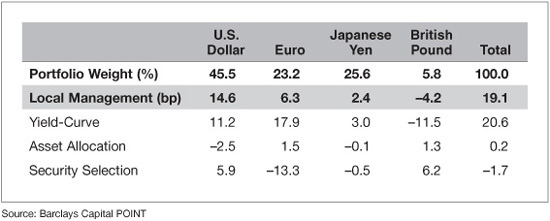
We can see that positive yield-curve outperformance came primarily from the U.S. dollar and the euro markets, whereas the British pound curve exposure resulted in a loss of –11.5 bp. We also see that asset allocation was not a significant driver of performance. Security selection decisions within each local market were significant, although the net result across all currencies was small at –1.7 bp. In particular, the selections within the U.S. dollar and British pound portion of the portfolio contributed positively, +5.9 bp and +6.2 bp respectively, but the selections within the euro portion of the portfolio negated these gains by contributing –13.3 bp.
Outperformance Due to Yield-Curve Exposure
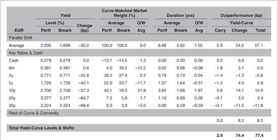
Focusing on the large yield-curve outperformance contribution, the manager wants to understand how her directive to go long duration by one year globally was implemented, and analyze the impact on each individual market. Exhibit 69–7 shows the yield-curve outperformance breakdown for the U.S. dollar portion of the portfolio.
EXHIBIT 69–7
Yield-Curve Outperformance Breakdown for U.S. Dollar

Individual market reports are unscaled by the value of the holdings in each market in order to evaluate single-market managers on an equal basis. Looking at each market in absolute terms allows us to reveal useful information about the management within each market, even for markets that constitute a small portion of the overall portfolio and their contributions to total portfolio outperformance are not significant. To translate the absolute unscaled numbers contained in the local reports into their contributions to total portfolio outperformance, one has to multiply such numbers by the corresponding market weight in the portfolio. In this example, the currency weights can be found in the Global Outperformance by Currency report in Exhibit 69–6; they are 45.5% for the U.S. dollar, 23.2% for the euro, 25.6% for the yen, and 5.8% for the British pound market.
The yield-curve report in Exhibit 69–7 contains a lot of information, but the manager can quickly see that the U.S. Treasury curve experienced bull-flattening with long rates falling in excess of 40 bp (third column from the left). She can also see that the portfolio is generally long duration by about 0.5 years (4.66 vs. 4.18). This is consistent with the general desire to be long duration, and with rates generally falling, it creates outperformance. More precisely, the yield change at the average maturity point of the benchmark is –31.6 bp. Multiplied by the (negative of) the average duration overweight of 0.48 years results in approximately +15.2 bp of outperformance contribution. The daily algorithm calculates that this number is actually +14.6 bp (top of the second to last column) by taking into account that duration exposure fluctuated during the period. The total U.S. dollar curve outperformance, accounting for the re-shaping of the yield-curve and the contributions from carry, is calculated to be +24.6 bp. Most of the additional outperformance comes from a butterfly position on the curve, where an overweight of the 20 year point of about 1.36 years is partially offset with under-weighting the 5, 10, and 30 year points. Since the 20 year point is the one with the largest yield drop (–48.7 bp), this butterfly position results in additional outperformance. The algorithm calculates and reports the excess contribution of each curve point separately.
The manager should be concerned that such a large component of total outperformance comes from an inadvertent position in the re-shaping of the U.S. curve (about +4.7 bp, estimated as the non-parallel U.S. curve outperformance 24.6 – 14.3 = +10.3 bp, times the U.S. dollar market weight of 45.5%) and should seek to control exposure to the various parts of yield curves more carefully.
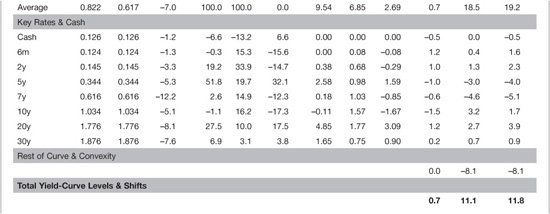
Exhibit 69–8 displays the yield-curve reports for the other three currencies. The euro curve outperformance analysis is very similar to the U.S. dollar one. There is duration overweight of about 1 year, as well as a butterfly position. Like the U.S. dollar curve, the euro curve also bull-flattens, resulting in (unscaled) outperformance of +77.4 bp and a contribution to total outperformance of +17.9 bp (remember that the average portfolio weight of the euro market is 23.2%). The yen has an even bigger duration overweight, about 2.7 years, but the curve movement is not as dramatic, with average yields falling about 7 bp. The portfolio contains significant curve reshaping positions as well, with the 20 year point being overweighted by more than 3 years, while the 20 year point is under-weighted by about 1.7 years. Nevertheless, the yen curve change is not sufficiently pronounced and generates only +11.8 bp of (unscaled) outperformance, contributing +3.0 bp to the total outperformance (the average portfolio weight of the yen market is 25.6%). The picture is completely different for the British pound. Here, the portfolio has a significant duration underweight of about 3.8 years, combined with a strong bull-flattening move of the British pound yield-curve (a yield change of –44.9 bp at the long end). This underweight results in a dramatic (unscaled) underperformance of –199.2 bp. The small average portfolio weight of the British pound market (5.8%) prevents this from being a major drag in the portfolio performance but even so its contribution to total outperformance is a significant –11.5 bp.
EXHIBIT 69–8
Yield-Curve Outperformance Breakdown for Euro, Japanese Yen, and the British Pound

At this point, it should be clear to the portfolio manager that understanding and managing the detailed exposure to the yield-curve of each currency is of paramount importance for proper control of the portfolio performance. She may also decide that global curve management is so important that it has to be managed before any local allocation and management decisions are made. In this case, a different attribution algorithm must be used, one that excludes yield-curve outperformance from the Local Market Allocation and Local Management Components. A detailed discussion on this type of analysis can be found in Chapter 71.
Asset Allocation and Security Selection
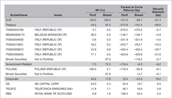
The manager now shifts her attention to the remaining sources of outperformance. First, she wants to understand how her views on the performance of U.S. assets panned out. From the “Global Outperformance by Currency” report of Exhibit 69–6, she already knows that U.S. dollar asset allocation contributed –2.5 bp to total outperformance. Exhibit 69–9 displays the U.S. Dollar Asset Allocation report, where we can see that most of the underperformance is caused by the overweight to corporate bonds. Remember that all numbers in this page are un-weighted; that is, they have to be scaled by the 45.5% portfolio weight of the U.S. market allocation in order to convert them into contributions to total portfolio outperformance. In particular, the 5% overweight sought to U.S. corporate bonds during the portfolio construction is represented here as an overweight of 10.9% (30.9% – 19.8% = 11.1%, approximately equal to 5%/45.5%), and the –2.5 bp of underperformance is reported as –5.5 bp (approximately equal to –2.5 bp/45.5%). The corporate sector contributes –5.2 bp, something that can be explained by the significant underperformance of the corporate sector in the benchmark (–70.2 bp) relative to the benchmark itself (–22.0 bp). The approximate calculation results in 11.1% × (–70.2 + 22.0) = –5.35 bp, close to the –5.2 bp reported. The Treasury and government-related sectors have no contribution to asset allocation, as their weights are matched exactly between the portfolio and the benchmark, as designed. Finally, the securitized sector has minimal contribution to asset allocation, despite the significant underweight, because its performance (–19.0 bp) is close to that of the benchmark (–22.0 bp).
EXHIBIT 69–9
U.S. Asset Allocation Breakdown
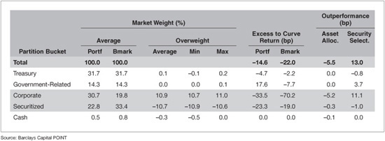
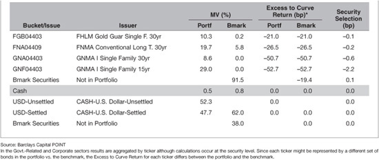
The same report also lists the contribution of each sector to security selection. We see that once again, the corporate sector is the dominant contributor with +11.1 bp out of the total +13.0 bp of security selection in the U.S. dollar market. To further understand the sources of security selection outperformance, the manager studies the detailed U.S. Dollar Security Selection report displayed in Exhibit 69–10. This report lists the chosen securities in each sector and their excess-of-curve return. We can see that the manager responsible for security picks in the U.S. corporate sector has indeed picked mostly securities whose excess returns beat the benchmark. One notable exception is the 6.45% 2037 Comcast bond, which represents 10.1% of the portfolio holdings in this sector (an overweight of 10% versus the benchmark) and which experienced –280.0 bp of excess return (much worse than the benchmark, which lost only 70.2 bp).
EXHIBIT 69–10
U.S. Security Selection Breakdown
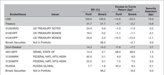
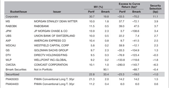
To estimate the contribution of the bond to the security selection outperformance coming from U.S. corporate bonds, one must take into account the weight of the corporate sector in the U.S. portfolio, which is 30.7%, to get 30.7% × 10% × (–280.0 + 70.2) = –6.4 bp. After scaling by the 45.5% weight of the U.S. portfolio, we calculate the contribution of the particular Comcast bond to global outperformance as 45.5% × –6.4 bp = –2.9 bp. This is quite significant and highlights the importance of name selection in a portfolio with a relatively small number of positions.
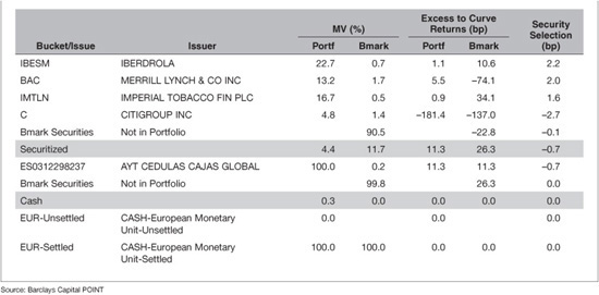
The manager also takes a look at the details of security selection in the euro market, which, as reported in Exhibit 69–6, reduces the total outperformance by a significant 13.3 bp. The report in Exhibit 69–11 lists the security selection outperformance as –57.4 bp (which scaled by the market weight of the euro market of 23.2% is equal to –13.3 bp) and identifies Italian government bonds as the main culprits. The fact that, absent any specific direction otherwise, the euro government sector was constructed by mostly Italian government bonds, leading to significant underperformance because of sovereign credit deterioration in Italy, indicates that the manager should attempt to take control of country exposure within the euro sector.
EXHIBIT 69–11
Euro Security Selection Breakdown
By now, the manager has a good understanding of most major contributors to the outperformance of the portfolio and has also reached some useful conclusions regarding the management of a small global portfolio.
• Yield-curve exposure is the dominant risk factor and must be managed explicitly in each currency.
• It is not sufficient to manage yield-curve exposure using just the duration. Exposure to curve re-shaping must also be controlled carefully.
• It may make sense to manage yield-curve exposure globally and not allow it to be determined by local allocation and management decisions.
• Name risk is very significant in a small portfolio; exposure to corporate issuers must be scrutinized and questionable names should be excluded.
• Country risk in certain areas such as the euro-zone must be managed separately.
Further insight can be gained by using a mode of performance attribution in which returns and outperformance are fully decomposed using all available analytics from pricing models. In this model, any part of outperformance that cannot be explained by analytics is reported as residual. This Fully Analytical model will be explained in detail in Chapter 70. Using this model, we get the local management details shown in Exhibit 69–12.
EXHIBIT 69–12
Local Market Management Details from a Fully Analytical Model
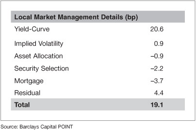
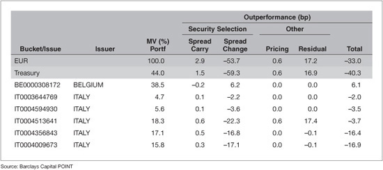
Comparing it with the report of Exhibit 69–3 we see that Local Market Management Details panel has changed. While the yield-curve contribution remains at +20.6 bp, asset allocation is now –0.9 bp instead of +0.2 bp, and security selection is now –2.2 bp instead of –1.7 bp. New terms have appeared, in particular Implied Volatility with +0.9 bp contribution, Mortgage with –3.7 bp contribution, and Residual with a prominent +4.4 bp. The Fully Analytical model also offers more clarity into sources of outperformance beyond the yield-curve, allowing users to understand the sources of the various types of outperformance; it will be discussed in detail in Chapter 70. In this example we will review only the Euro Security Selection report shown in Exhibit 69–13. We can see that not only is the portfolio concentrated on Italian government bonds, but that it also contains bonds of very long maturity, further overweighting the entire European government sector in terms of spread duration exposure. This may lead the manager to draw yet another conclusion: The spread duration exposure of sectors with credit risk must be carefully controlled.
EXHIBIT 69–13
Euro Security Selection Report
Performance Attribution as a Data Quality Tool
A comprehensive and detailed performance attribution system serves as a magnifying lens for data quality problems and allows users to pinpoint and correct such issues quickly.
The report of Exhibit 69–13 shows that one particular Italian government bond (Issue IT0004513641) is almost single-handedly responsible for the entire reported residual. Indeed, it contributes +17.4 bp of residual to the euro portfolio, which, when scaled by the euro portfolio market weight of 23.2%, results in +4.0 bp of portfolio-level residual (out of the total of +4.4 bp reported in Exhibit 69–12). A diligent manager will promptly investigate such residuals. They may mean one of the following four things:
• Incorrect total returns. This can be caused by missing or incorrect prices, transaction errors, incorrect corporate actions, etc.
• Missing or inaccurate analytics produced in the security valuation process
• Attribution model deficiencies wherein certain contributing factors are not captured by the factor return decomposition
• Issues with the attribution algorithm or its implementation
All four are extremely important for the portfolio manager to know. Over time, model deficiencies will presumably be corrected, leaving data quality problems in the form of bad returns or bad analytics to be the primary cause of attribution residuals.
In the case of this portfolio, a quick investigation reveals that the offending bond had a coupon payment of 2.50% that has been recorded twice. The price of the bond on the coupon payment date was approximately 110; therefore, one would expect a residual of +227.3 bp at the bond level. Indeed, after taking into account the net weight of the bond, the residual contribution of the bond to the euro portfolio is 44.0% × (18.3% – 0.5%) × 227.3 = +17.8 bp, very close to the +17.4 bp of reported residual. Re-running the report after correcting the double entry produces a mostly identical report (Exhibit 69–14) to the one before (Exhibit 69–12), except that the return of the portfolio is lower by the correction amount (+4.2 bp), the outperformance is +34.5 bp instead of +38.7 bp, and the residual term has been reduced correspondingly from +4.4 bp to +0.2 bp.
EXHIBIT 69–14
Results from the Fully Analytical Model after the Data Correction

Data problems have the potential to affect the quality of outperformance measurement of a portfolio significantly, as well as its breakdown to the various sources. Proper use of an analytics-based attribution platform can help identify and correct potential issues promptly.
KEY POINTS
• Performance measurement and attribution is an important function of the investment process. It helps bring clarity to the sources of portfolio risk and performance and identify the contributions of individual decision-makers.
• A successful performance attribution algorithm should satisfy three important requirements: additivity, completeness, and fairness.
• A good attribution system should have a calculation and compounding frequency that corresponds to the dynamics of modern portfolio management. This normally means daily frequency for an actively managed fixed income portfolio.
• A good attribution system should have the flexibility to accommodate the wide range of portfolio management styles. The best attribution is an analysis that best matches the portfolio management decision making process.
• Performance attribution algorithms typically follow either a sector-based allocation or a factor-based allocation, but neither is sufficient to cope with the complexity of modern portfolio management.
• Algorithms that combine the sector-based and the factor-based attribution have the flexibility to adapt to the particular management structure of most fixed income and equity portfolios.