CHAPTER
SEVENTY
PERFORMANCE ATTRIBUTION FOR PORTFOLIOS OF FIXED INCOME SECURITIES

ANTHONY LAZANAS, PH.D.

Managing Director
Barclays Capital

ANTÓNIO BALDAQUE DA SILVA, PH.D.

Director
Barclays Capital

CHRIS STURHAHN

Vice President
Barclays Capital

ERIC P. WILSON

Vice President
Barclays Capital

PAM ZHONG, CFA

Vice President
Barclays Capital

In contrast to the simple and opaque nature of equities, fixed income securities can be thought of as structured investments which promise to pay a stream of cash flows. The magnitude of cash flows can be fixed, or may depend on observable variables (e.g., realized inflation, principal prepayments of mortgage loans, or the price of the security itself for securities with call/put features). This quasiformulaic nature of fixed income securities allows their present value to be expressed as a (generally stochastic) function of economic variables—most prominently interest rates and credit spreads—which can be calibrated to observed market prices of reference securities to generate a “pricing model.” In other words, a pricing model is a function that expresses the present value of a fixed income security (or derivative contract) as a function of economic variables. This function can be also used to estimate the sensitivities of the present value to changes in the underlying variables. Such sensitivities, generically called analytics and known as greeks in the options world or duration/convexity in the bond world, can and are being used as loadings to the pricing factors driving returns during performance decomposition and attribution of fixed income portfolios.

The authors would like to thank Lev Dynkin for introducing us to the concept of performance attribution, Jay Hyman for many insightful ideas over the years and Attakrtit Asvanunt who was instrumental in the development of many concepts in this chapter.

In this chapter we discuss in detail how the performance of a portfolio of fixed income securities relative to a benchmark can be analyzed using the hybrid performance attribution algorithm described in the Chapter 69. The hybrid methodology that combines factor-based attribution with the traditional Brinson method is particularly appropriate for fixed income securities whose return usually includes a significant component driven by a common factor, interest rates. In this chapter, we will focus on attribution over a single period only. As discussed in Chapter 69, a single period is one business day for the majority of fixed income systems. Methods for compounding single period attribution results over longer periods of time will be discussed in detail in Chapter 71.

We begin the discussion by using a generic pricing model in order to split the return of a fixed income security into the contributions of the various factors driving the security return. We discuss in detail the treatment of the most important factors such as interest rates, implied volatility and credit spreads. Two important asset classes with special characteristics, mortgage-backed securities and inflation-linked bonds, are discussed separately. We then show how the flexible hybrid attribution framework can be applied in several ways to accommodate various types of fixed income portfolios and styles of portfolio management.

In this chapter we restrict the analysis to single-currency portfolios. The complications arising from investing in multiple currencies will be discussed in the Chapter 71. All performance attribution reports have been generated using the Barclays Capital Hybrid Performance Attribution (HPA) model¹ as implemented in POINT, the Barclays Capital portfolio analytics and modeling platform.²

RETURN SPLITTING

Securities with deterministic cash flows are priced by discounting the cash flows off a reference yield-curve. When future cash flows are not known but can be reasonably predicted by modeling them as functions of economic variables (most commonly interest rates) and security characteristics, more complex statistical diffusion models are used. Such models produce a set of projected interest rate paths that are consistent with the current yield-curve and the market implied volatility of liquid interest-rate options. Projected cash flows on each path are discounted at the corresponding discount factors, and the present value of the security is calculated as the average present value across all interest-rate paths. In this case, the present value of a security is a function of interest rates, their implied volatility and possibly other variables in the model.

A pricing model produces the “model value” of a security. In the case of securities such as derivatives that are traded over-the-counter, the model value is usually used to mark-to-market positions in the security. When a security is publicly traded, its market price generally does not agree with the model price. To make them equal, model parameters are calibrated to match the market price. For example, in the case of bonds, this usually entails additional discounting of cash flows at a flat rate across all maturities. In the majority of models, in which cash flows are discounted at a risk-free reference yield-curve (the government or swap yield-curve in a particular currency), this additional discounting rate is the well-known option-adjusted spread (OAS), which captures the extra discounting required to account for credit, liquidity and other types of risks. Analytics produced by such a model are therefore known as option-adjusted analytics.

Generically, a pricing model can be expressed with the following formula:

MarketValue = f (Time, YC, Vol, Other, OAS)

Here, YC stands for yield-curve, Vol for implied volatility, and Other for any other market factors or parameters that the pricing model is using.

For a single-currency portfolio, the analysis begins with splitting the return of each portfolio position into the contributions of various factors. Most pricing systems provide the first-order sensitivity of the market value of a position to the underlying risk factors. Sometimes second-order sensitivities to particular factors (such as interest-rate convexity) are also reported. Using these sensitivities, the return of a particular position is approximated as a linear combination of the contributions of each pricing factor, for example:

Although some pricing systems do provide additional sensitivities (e.g., spread convexity, or sensitivities to some of the “other” pricing factors such as prepayment speed for mortgage securities) most of the times the difference between the actual return of a position (as reported in the accounting system of the portfolio) and the above approximation is non-negligible. Such difference, usually referred to as Residual, is attributable to sensitivities to unaccounted model inputs and parameters, higher-order terms, cross-terms between factors, and very often in practice, data and calculation errors. Analyzing the residual and understanding whether it is legitimate or a result of data or calculation error is an important function of a performance attribution system. To help achieve that, sophisticated performance attribution systems use an alternative scenario-based decomposition of returns, which by design is complete, i.e., has no residual. The return splitting exercise in such systems has two stages:

Stage I: Scenario-based return decomposition into broad categories

Stage II: Analytics-based return decomposition into fine categories

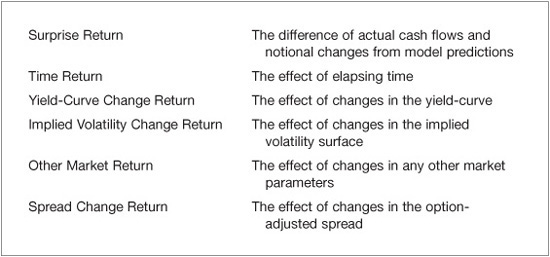
In Stage I, the scenario decomposition of one-period return³ begins with the market value of the position at the beginning of the period and then moves one parameter at a time to the end-of-period value until all of the parameters have changed and the end-of-period market value is obtained. At each step, the market value of the security is obtained by fully recalculating its market value by changing one input parameter at a time. This stage divides the return into broad categories, as described in Exhibit 70–1.

EXHIBIT 70–1
Typical Scenario-Based Return Decomposition

Of course, this is not the only possible decomposition. Coarser or finer decompositions are also possible, but this particular one is a good compromise between computational complexity and informational content for most fixed income portfolios. In Stage II, the sensitivities of the security to various pricing model inputs (analytics) are used to decompose the return further. The combination of the two decompositions allows the residual to be split among the major return constituents providing more insight about its potential sources.

We will now discuss in more detail the various return constituents in the typical decomposition of Exhibit 70–1.

Surprise Return

Surprise return is relevant to securities whose cash flows and amount outstanding are not deterministic. For example, for mortgage-backed securities, it is prepayments that generate the random behavior of cash flows and amount outstanding; for inflation-linked securities, it is the dependence of cash flows on the reference inflation index. Security valuation models make assumptions about inputs to pricing models and use such projections to value securities until realized values are known. The return explained by running scenarios or using model analytics is the return that would be realized if the uncertain parameters were consistent with the model predictions. If the realized values of the parameters are different from the projected ones, the difference between the actual return and the return explained by the model is captured as surprise return.

Mortgage Prepayments Surprise Return

As an example, consider a mortgage-backed security that is trading at a price of 105 and zero accrued. The prepayment model projects a 2.4% prepayment over the next month (25% CPR), thus predicting a return due to prepayments of –11.4 bp.⁴ If the actual prepayment is lower, say 1.3% (15% CPR) resulting in a prepayment return of –6.2 bp, the difference of +5.2 bp will be registered as prepayment surprise return. The model-expected –11.4 bp of prepayment return will be part of the time return component.

Inflation Surprise Return

As another example, consider an inflation-linked security that is trading at a price consistent with projected inflation for next month of 3.0%. If the actual inflation announcement is 3.5% it will give +4.2 bp⁵ of inflation surprise return to account for the larger inflation accretion accumulated over the month relative to the projected inflation rate. This return is separate from any return resulting from presumably increased future inflation expectations caused by the higher-versus-expectations announcement. Such return is captured separately as inflation spread change as will be described below.

Time Return

Time return is the deterministic component of the return, i.e., the return predicted by the pricing model if market parameters remain unchanged.⁶ For most fixed income securities, time return can be decomposed into yield-curve carry, spread carry and volatility decay. Inflation-linked securities also have inflation accretion and inflation spread carry. These time return components can be measured using analytics, as we will describe in detail in following sections.

Yield-Curve Change Return

Changes of interest rates affect securities returns primarily through the change of discount factors. In addition, some securities have cash flows that are modeled as functions of interest rates (mortgage-backed, floating-rate securities). The component of return that is due to the fluctuation of the yield-curve is captured by the yield-curve change return component. The exposure of the security value to the yield-curve is captured by its sensitivity to parallel shifts of the yield-curve, the option-adjusted duration (OAD), movements of a specified set of points (key-rate points) representing the yield-curve, the key-rate durations (KRDs), and its second-order sensitivity, option-adjusted convexity (OAC). In daily frequency attribution models the potential daily change of yields is limited (moves above 15 bp are very uncommon); therefore, the convexity contribution is typically much smaller than the duration contribution. For this reason, the effect of yield-curve convexity does not need to be explicitly measured.⁷

Yield-Curve Change Return Decomposition

How total yield-curve change return is broken down between duration and convexity depends to a large extent on the frequency at which the duration exposure of a portfolio is managed. In this example a daily frequency is assumed, consistent with the practice of the majority of portfolio managers. To understand the frequency implications, consider a portfolio with interest-rate duration of 5 and an interest-rate convexity of –2. Assume that over the two weeks, interest rates keep falling at 10 bp per business day for a total of 100 bp. The duration-convexity formula explains portfolio returns caused by changes in interest rates:

where both the returns and the rates change are expressed in basis points.

Applying this formula for the entire two weeks results in the following:

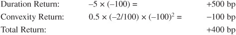
On the other hand, applying the formula daily generates quite a different breakdown. The daily algorithm must take into account additional complexities such as the duration drift of the portfolio, as well as compounding. It is not sufficient to simply calculate the daily duration and convexity return as –5 × (–10) = +50 bp and 0.5 × (–2/100) × (–10)² = –1 bp, respectively, and just aggregate over 10 days to get +500 bp duration return and –10 bp convexity return, for a total return of +490 bp. Instead, the daily duration drift of the portfolio due to falling interest rates must be estimated first. Using the definitions of duration and convexity, the duration change due to a change in interest rates can be estimated as:

ΔOAD = (OAD² Δ 100·OAC) · Δr/10,000

where duration and convexity have the usual units and change of rates is measured in basis points. Due to the high convexity of the portfolio, over the course of the 10 days the duration of the portfolio shrinks by about 2 years. In addition, both the total return of the portfolio and the contributions of duration and convexity must be compounded daily (see Chapter 71 for details). After both adjustments, the total return calculation and breakdown are as follows:

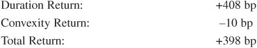
The total return is very close to the one estimated by analytics at the beginning of the period, but the breakdown between duration and convexity is dramatically different. In the daily model, the convexity contribution is much smaller than the duration contribution.

Daily attribution models typically use only the key-rate durations to explain the contribution of yield-curve changes. Any yield-curve change return (as estimated by the scenario-based total yield-curve change return) in excess of what can be explained by the key rates captures the contribution of the yield-curve movements between the key-rate points, as well as the convexity and other second-order terms and can be reported separately.

Implied Volatility Change Return

Securities with optionality require reference implied volatilities to calibrate the interest rate diffusion pricing model. In the fixed income world, most models use the Black swaption implied volatility surface⁸ as input and calculate the sensitivity of the security value to the changes in implied volatility with a single analytic, Vega, which is the price change of the security for a 1% parallel shift in the Black implied volatility surface. Vega does not capture the effects of non-parallel movements of the implied volatility surface or the effect of yield-curve moves on the diffusion parameters of the interest-rate diffusion model.⁹ Clearly, it does not sufficiently represent the sensitivity of the security value to changes in implied volatility surface. Some advanced models are capable of generating partial Vegas, e.g., sensitivities to exposures at multiple points of the volatility surface, or, alternatively, to a vector of parameters that can be used to parametrically fit the volatility surface. In such cases a more detailed decomposition of implied volatility change return is possible.

If only parallel Vega is available, capturing the total effect of implied volatility changes through scenarios is imperative. The scenario-based implied volatility change return can then be decomposed into a parallel shift component that is equal to the product of Vega and the average volatility shift, and a remainder that contains the effects of nonparallel volatility movements as well as the effects of changes of other inputs and parameters used in the volatility model.

Other Market Return

Although yield-curve and implied volatility are the most important factors in the pricing models of most fixed income instruments, they do not capture every aspect of the cash flows, and more factors may be required. Securities or derivatives with cash flows that depend on external factors, such as prepayments or inflation levels, may use additional inputs to the pricing model. Changes in such inputs will generate return that is not attributable to yield-curve or implied volatility surface changes. The effects of the changes of all others factors are captured together as Other Market Return.

For example, the model-projected cash flows of mortgage-backed securities may depend on market mortgage rates, as well as additional model-specific parameters such as home price appreciation expectations or swap spreads. All of these parameters contribute to Other Market Return. The breakdown to the various factors follows an instrument specific algorithm and depends on the availability of specific analytics.

Spread Change Return

The effect of OAS changes to return is captured in the spread change return component. Sensitivity to spread movements is measured directly using both spread duration (OASD) and spread convexity (OASC). The large spread moves often observed in the market make it necessary to use spread convexity. The difference between the sum of spread return captured by OASD and OASC and the scenario-based spread return contributes to the residual return component.

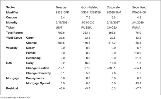
Reporting the return split of individual securities and sectors in a portfolio and a benchmark is very useful for the portfolio manager as it provides a detailed understanding of the sources of exposures and returns in the portfolio. When reporting return splits, attribution systems may re-organize the various components of returns. In particular, the Barclays Capital HPA model which we use for illustrations in this chapter, re-groups the return components along risk-factors as shown in Exhibit 70–2. Sample return splits for a few securities can be found in Exhibit 70–3.

EXHIBIT 70–2
Return Splitting Components

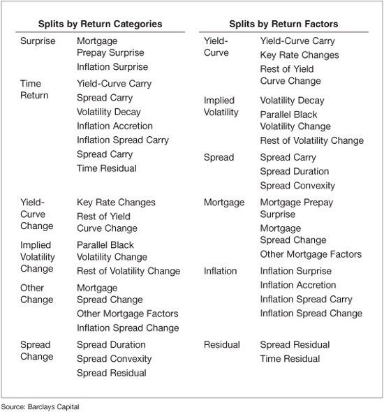
EXHIBIT 70–3
Security Return Splits

OUTPERFORMANCE BREAKDOWN

Having split the returns in such detail based on analytical exposures to market factors, one might be tempted to proceed with bottom-up aggregation of outperformance per factor. However, neither does every portfolio manager use the factor approach to management, nor do all agree on which factors should represent portfolio risk. Many portfolios are managed by sectors or asset classes where top-down decomposition of outperformance is more appropriate, as the returns of the portfolio and the benchmark in each asset class or sector may differ. A flexible hybrid approach for performance attribution can be useful for both methods by allowing users to flexibly split total return into two parts: that driven by common factors for the entire portfolio and that in excess of common factors, which is further explained by asset allocation/security selection based on a user-defined hierarchical partition of the investment universe into sub-universes that we will refer to with the term “partition buckets.”

Common components are explained by bottom-up aggregation as the difference of the exposure of the portfolio and the benchmark multiplied by the factor return. For example, yield-curve exposure is captured by duration, thus the outperformance explained by yield-curve movement would be the duration overweight of the portfolio (over the benchmark) multiplied by the negative of the yield-curve change. Excess of common or allocated components is explained by top-down decomposition using a user-defined hierarchical partition and the recursive algorithm discussed in Chapter 69, as will be detailed below.

This approach has the ability to accommodate different portfolio management styles. It also allows users to compare different ways of analyzing returns and outperformance and can lead to a better understanding of what drives portfolio outperformance. For example, many high-yield managers do not like to split total return into yield-curve, implied volatility and spread components, citing the high negative correlation between yield-curve and implied volatility return versus spread return. Instead, they prefer to manage total return as a whole. And even when they do wish to separate out yield-curve return and manage the excess-to-yield-curve return, they usually do not rely on spread duration and spread convexity to measure their exposure. However, when spreads were very tight in 2005, many high-yield managers began experimenting with spread duration-based management.

While any return split component could be considered as a bottom-up common return component or as an excess return component that participates in the top-down allocation algorithm, the following three common configurations support most portfolio management decision-making structures: Total Return Model, Excess Return Model, and Fully Analytical Model.

The Total Return Model is the simplest model, where the total return is considered a single allocated factor. In other words, there is no common factor, and the total return is explained by top-down decomposition using market value weights and a user-defined security partition.

The Excess Return Model takes advantage of the return splitting algorithm to separate the factors contributing to return into common and allocated factors. Returns from common factors are explained by bottom-up aggregation using appropriate analytic weights (e.g., OAD, Vega, market beta, and the like.). For fixed income portfolios yield-curve and/or implied volatility are typically considered as common factors. Returns from other factors (excess-over-common factor returns) are explained by top-down decomposition as in the Total Return Model.

The Fully Analytical Model is the most detailed model. It takes full advantage of the return splitting algorithm and the hybrid allocation algorithm, where each factor can be explained either by the top-down or the bottom-up aggregation using appropriate weights.

The following sections discuss these different types of models in more detail.

TOTAL RETURN MODEL

The Total Return model is the most basic performance attribution model and follows the classical, sector-based, asset allocation/security selection framework. It is appropriate for portfolios whose managers make decisions solely based on the total returns of the securities. A typical usage is a portfolio whose managers are allocating the capital based on their views of the sector and security returns, rather than risk factors. The model is generic in that the allocation buckets can be defined via a user-defined partition using any of the hundreds of security attributes available. Allocations such as geography, size, and momentum can be used, essentially mimicking factor-based allocation. The partition should be defined to mimic the management structure of the portfolio.

The Total Return model uses the relative allocation method of the top-down decomposition algorithm as explained in Chapter 69, where sector market value weight w_s is the allocation weight α_k,s, total return of sector s is the only factor return f_{k, s}, and total return of the benchmark is the hurdle rate.

Absent leverage, the top-level weights of the portfolio and the benchmark are both equal to one, so the top-level exposure term is always zero.

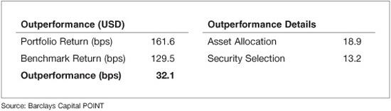
Let us now re-visit the attribution example of the Chapter 69 to illustrate how results change according to the attribution model used. We remind the reader that in Chapter 69 we analyzed the outperformance of a multi-currency portfolio versus the Barclays Capital Global Aggregate G4 Index over a period of one month. Here, we will focus only on the U.S. Dollar portion of the portfolio which achieved a +32.1 bp outperformance¹⁰ versus the U.S. Dollar portion of the index.

Using the Total Return model and assuming that the asset allocation universe consists of the major asset classes in the U.S. Dollar fixed income markets, the total portfolio outperformance is split into +18.9 bp of asset allocation and +13.2 bp of security selection as shown in Exhibit 70–4.

EXHIBIT 70–4
Outperformance Breakdown Using the Total Return Model

The contribution of each asset class to both asset allocation and security selection is calculated based on the total return of each asset class in the portfolio and the benchmark using Eqs. (70–1) and (70–2) and reported in Exhibit 70–5.

EXHIBIT 70–5
Asset Allocation Using the Total Return Model

The corporate sector contributes +7.4 bp to the outperformance, since it has been overweighted by about 10.9% (portfolio average weight: 30.7%, benchmark average weight: 19.8%) and its performance in the benchmark (+196.1 bp) is much higher than the performance of the benchmark itself (+129.8 bp). The approximate¹¹ calculation yields 10.9% × (196.1 – 129.8) = +7.2 bp, close to the +7.4 bp reported. The contribution to security selection is also shown and captures the performance advantage of the portfolio versus the benchmark, weighted by the portfolio weight of each sector. For the corporate sector, this calculation yields 30.7% × (107.9 – 196.1) = –27.1 bp, close to the –27.3 bp reported.

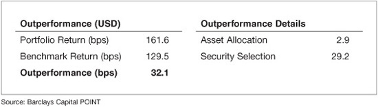
The analysis above assumed that asset allocation occurs only at the major asset class level (Treasuries, Government-Related, Corporates, Securitized, and Cash). It is likely that within each major asset class a second level of allocation to asset class subsectors will occur. For example, within the Securitized sector further allocation to the Residential Mortgages (RMBS) sector, the Commercial Mortgages (CMBS) sector, the Asset-Backed (ABS) sector, and Covered Bonds may be desirable. As discussed in Chapter 69, a flexible attribution algorithm should support multiple decision levels. In our example, we introduce a second level of asset allocation by using asset class subsectors as defined by the Barclays Capital Global Aggregate Index classification scheme. In this case the Total Return model applied recursively reports a dramatically different breakdown between asset allocation and security selection as reported in Exhibit 70–6. Asset allocation shrinks from +18.9 bp to +2.9 bp, while security selection grows from +13.2 bp to +29.2 bp.

EXHIBIT 70–6
Outperformance Breakdown Using the Total Return Model (Two-Level Asset Allocation)

Intuitively, the finer the partition used for asset allocation the more emphasis is put on asset allocation decisions versus security selection decisions. In the limit, if the buckets of the asset allocation partition are individual securities, then the entire outperformance is reported as asset allocation. Conversly, if the asset allocation partition contains only one bucket, the entire outperformance is reported as security selection. Notice though that the transition between the two limits is not monotonic since individual partition buckets may contribute positively or negatively to both asset allocation and security selection. Such flexibility to define the asset allocation levels used in the breakdown of total outperformance is an important characteristic of an attribution system as it can support multiple styles of portfolio management. It is important that the partition used for performance attribution corresponds to the decision structure used for the management of a particular portfolio.

To understand the differences between single-level and two-level asset allocation, examine the two-level asset allocation details shown in Exhibit 70–7. In the Level-1 report, there are two columns for asset allocation, a top-level one (labeled simply Asset Allocation) which is identical to the asset allocation from the simple partition (+18.9 bp) and a Further Allocation column that captures subsequent allocation decisions (–16.0 bp). Their sum is +2.9 bp, the asset allocation reported in the summary report. Level-2 reports illustrate the details of the asset allocation into subsectors within each of the major asset classes. Asset classes for which no subsectors are defined (such as Treasuries and Cash) do not get Level-2 reports and do not contribute to Further Allocation.

EXHIBIT 70–7
Two-Level Asset Allocation Using the Total Return Model

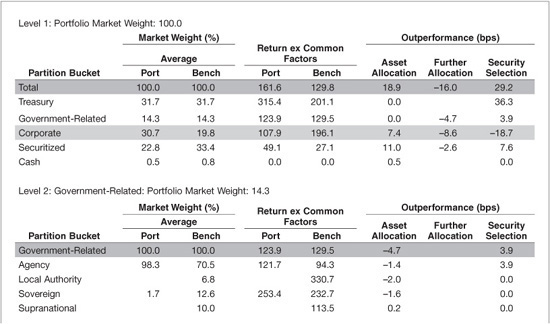
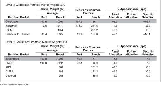
Let us focus again on the corporate sector which shows –8.6 bp of underperformance contribution from Further Allocation. Its Level-2 decomposition table explains why: the portfolio had a large overweight to financial institutions, an underweight to industrials and no allocation to utilities. While both industrials and utilities outperformed the corporate benchmark, financials had a lower performance of +157.0 bp than the +196.1 bp of the aggregate corporate sector. Therefore, all three sectors have negative contribution to outperformance, with the largest (–5.1 bp) coming from financial institutions. Once again, this can be approximated with the recursive application of Eq. (70–1) as follows: 30.7% × (80.4% – 38.5%) × (157.0 – 196.1) = –5.0 bp close to the –5.1 bp reported. The security selection numbers represent security selection within each sub-sector.

EXCESS RETURN MODEL

The Excess Return model uses the return splitting algorithm to extract common factor returns from the total return and considers the remainder as excess return. In the fixed income world, portfolio managers like to manage their exposures to common factors such as the movement of the yield-curve and implied volatility surface separately from their other investment decision choices. For example, consider a manager who chooses to hedge the overall exposure to the yield-curve and makes investment decisions purely based on expectations of excess-to-curve returns. In this case, she would like to see the total outperformance breakdown into yield-curve and excess return so that she can assess the effectiveness of the hedge, as well as the asset allocation/security selection choices separately.

The outperformance due to exposure to common factors, which we will discuss in detail below, is explained by bottom-up aggregation. The excess return outperformance is explained by top-down decomposition using the relative allocation model of the Chapter 69, with sector excess returns and sector market value weights as in the Total Return model.

Once again, if neither the portfolio nor the benchmark is leveraged, the top-level weights are equal to one and the top-level exposure term is equal to zero.

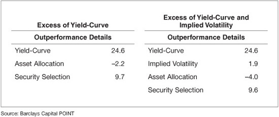
Exhibit 70–8 shows the outperformance breakdown when using the Excess Return model and the two-level asset allocation in the previous example. The left-hand side table shows the results when only interest rates are treated as common return factors. Most of the outperformance (+24.6 bp) comes from the yield-curve exposure. Asset allocation is responsible for –2.2 bp and security selection for +9.7 bp. The right-hand side table shows the results when, in addition to interest rates, implied volatility is also treated as a common factor. The Implied Volatility term contributes +1.9 bp to outperformance, altering the asset allocation contribution to –4.0 bp and the security selection contribution to +9.6 bp.

EXHIBIT 70–8
Outperformance Breakdown Using the Excess Return Model

Outperformance Due to Yield-Curve Exposure

As discussed at the beginning of this chapter, the pricing framework for most fixed income securities essentially amounts to projecting future cash flows and discounting them at projected paths of interest rates. Government, swap, or municipal AAA interest rate yield curves can be used as the reference yield-curve, depending on the type of the security.

The yield-curve contribution to outperformance includes yield-curve change, the effect of interest rate changes, and yield-curve carry, the effect of the change of yield-curve discount factors or interest rate-related projected cash flows with the passage of time assuming that rates stay unchanged. There exist two different philosophies with respect to the definition of what constitutes a change in interest rates, and they result in different breakdowns between yield-curve carry and yield-curve change; however, the total yield-curve effect (their sum) is identical under both methodologies.

Methodology I: Rolling on Forwards

A yield-curve is deemed unchanged if the rates realize the values implied by the forward rates in the previous period. For example, if we look at an unchanged yield-curve one month into the future, the 1-year rate is equal to the one month forward 1-year rate calculated from today’s yield-curve. In this methodology, a yield-curve change is calculated with respect to the projected forward rates, and carry always accrues at the short rate.

This method is not very popular (particularly among cash investors) because it introduces significant complexity in the estimation of yield-curve change return—the most important component of fixed income returns. In addition, forward rates are not particularly good predictors of the realized path of interest rates, further reducing the appeal of this method.

Methodology II: Parallel Translation

A yield-curve is deemed unchanged if the level and shape of the yield-curve remains unchanged. For example, if we look at an unchanged yield-curve one month into the future, the 1-year rate is equal to the 1-year rate in today’s yield-curve. In this methodology, a yield-curve change is calculated with respect to today’s yield-curve, and carry accrues at a different rate for each cash-flow.

Further, the representation of the yield-curve (e.g., par rates, zero rates, forward rates) is important and affects the breakdown of total yield-curve return between carry and change. If instantaneous forward rates are used to represent the yield-curve, then each cash-flow accrues carry at a rate equal to the forward rate corresponding to the cash-flow date. Securities with deterministic cash flows accrue carry at a rate equal to the average of the forward rates corresponding to the date of each cash-flow, weighted by the present value of each cash-flow. Unfortunately, the forward rate representation is not very popular since forward rates are not directly observable in the market. Investors prefer the better understood zero or par rates to represent a yield-curve. Under both representations, the calculation of the curve carry of a set of cash flows is complicated. From the discussion above it is evident that the breakdown of yield-curve return and outperformance into curve carry and curve change is somewhat subjective. Portfolio managers should have the flexibility to choose a methodology which is consistent with their style of management.

Since interest rate yield curves are infinite-dimension objects, we need to represent them with a finite set of parameters. The simplest method is to choose a small discrete set of yield-curve points (key-rate points) dispersed along the yield-curve. The premise is that the dynamics of the yield-curve can be represented with the dynamics of the key rates with a high degree of accuracy. Intermediate yield-curve points are assumed to move as a linear combination of the moves of adjacent key rates. A typical set of key rates used includes the 6-month, 2-year, 5-year, 10-year, 20-year and 30-year points for most currencies. Other curve points that also appear are the 1-month, 3-month, 1-year, 3-year, 7-year, 12-year, 15-year, 25-year and 40-year points. Some managers prefer to represent the curve using factors that are defined as linear combinations of curve points. The prototype for such representation is the level-slope-butterfly set of factors, a representation implied by the principal component analysis of yield curves. The choice of yield-curve representation depends on the type of yield-curve exposure a portfolio is taking as well as the capabilities of the underlying analytics system.

Although the key rates or level-slope-butterfly representation of the yield-curve is highly accurate from a risk perspective (captures more than 99% of its variance), there may be deviations from a return perspective, especially if a small number of points are used. Indeed, there are periods where, for example, the three-year U.S, Treasury rate moves very differently than what is implied from the two-year and five-year rates. Analytics (key-rate durations) explain the bulk of yield-curve outperformance. Scenario-based outperformance calculations are used to capture any residual outperformance from intermediate yield-curve points and convexity.

Yield-Curve Carry

As discussed above, yield-curve carry calculations are complex even for bullet securities under par- or zero-rate representation of yield curves. An approximation method for the calculation of yield-curve carry, called the Curve Matching Portfolio (CMP) method, can be used to simplify these calculations.

The basic idea is to define a set of par and/or zero-coupon reference bonds whose yield-curve carry can be easily computed analytically, and then construct a carry-matching portfolio of such bonds for each portfolio or benchmark security. The matching algorithm attempts to create a portfolio that earns the same yield-curve carry as the security.

Matching par bonds are made to have a coupon equal to the par key rate of the corresponding maturity and a price of par (100). The payment frequency and day count convention match those used for yield-curve construction. As a result, all matching par bonds on the day of construction have an option-adjusted spread of zero by construction. Zero-coupon bonds do not pay coupons, but have yields matching the zero rates for maturities matching each point.

A curve matching portfolio consisting of reference bonds and cash is created for each security in the portfolio and benchmark such that the cash-flow profile of the portfolio matches the one for the bond. Since dealing with bond cash flows (which are often nondeterministic) is generally difficult, some algorithms use key-rate durations to represent the concentration of cash flows around each key-rate point. Therefore matching the key-rate durations of the curve-matching portfolio and the bond is an approximate way to match their cash-flow profiles and thus the curve carry. Cash is added or subtracted from the matching portfolio to make sure that it has the same present value with the bond. The amount of cash needed to replicate any particular bond can vary according to the duration profile and price of the bond. For example, if only par bonds are used in the matching portfolio of a bond with a higher coupon than the current par rate, leverage must be used in the matching portfolio (borrowing at the short rate to fund the future cash flows) to match the cash-flow profile of the bond. This leads to a negative amount of cash in the matching portfolio.

A common choice for the set of matching reference bonds is to use one par or zero bond per key-rate point. The weights of each reference bond (and cash) are aggregated over all positions in the portfolio and benchmark. Let us represent with and weights allocated to reference bond and cash in the curve-matching portfolio of the portfolio and benchmark respectively, with j spanning all key-rate points and cash. If we approximate the carry return of each reference bond and cash as its yield (by definition the corresponding key rate level) multiplied by the attribution period length y_jΔt, the yield-curve carry outperformance can be broken down per key-rate point contribution as If we define the average portfolio or benchmark yield as the average of all key rates using the CMP portfolio weights, the above formula can be re-written as . The excess yield-curve carry contribution of each key rate over the average carry can be defined, but the sum over all key rates will be zero.

Generally, yield-curve carry can be broken down using the following equations:

If the average yield is set to zero for both portfolio and benchmark, then the average carry term is zero and the yield-curve carry outperformance is attributed to each key rate. If the average yield is calculated using the CMP weights for portfolio and benchmark, then the average carry is equal to the total carry contribution and the sum of the excess key rate contributions is equal to zero. Other choices for the average yield are also possible.

Yield-Curve Change

Yield-curve change outperformance is a result of duration profile differences between the portfolio and the benchmark and the change in the yield-curve. The scenario-based return decomposition described earlier is used to compute the total yield-curve change return and hence the outperformance. Then, by using the analytics (OAD and KRDs), the total yield-curve change outperformance is decomposed further into a parallel shift component, a curve reshaping (at the key-rate points) component, the rest of yield-curve contribution and the effects of convexity.

The outperformance from parallel yield-curve shift is computed by applying the bottom-up aggregation, using key-rate durations as loadings and key rate changes as factors. Similar to yield-curve carry, the notion of an average yield change (parallel shift) can be used to control how the yield-curve change outperformance is distributed between the key rate contributions and the parallel shift term.

If the average yield change is set to zero, the yield-curve change outperformance will be attributed to each key rate separately. If the average yield change is set equal to an appropriately defined parallel shift, the key rate terms capture the outperformance in excess of the parallel shift; i.e., the yield-curve reshaping effect on outperformance.

Since we represent the shape of the yield-curve by key-rate points, there will always be a small fraction of yield-curve change outperformance not captured by the above methodology, as explained at the beginning of this section. Exhibit 70–9 illustrates the change not captured by the key rates.

EXHIBIT 70–9
Approximation of Yield-Curve Change by Key Rates

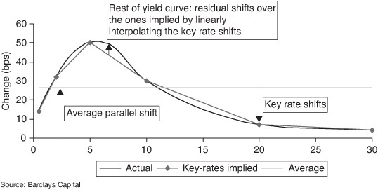
This final piece of the yield-curve change outperformance, calculated as the difference between total yield-curve change return from the scenario-based decomposition and the sum of the average parallel shift and reshaping return, includes the change in excess of key rates as well as return from convexity and other higher-order terms.

Exhibit 70–10 displays a yield-curve attribution report as produced by the Barclays Capital HPA model.¹² The total yield-curve outperformance of +77.4 bp is broken into +2.9 bp of curve carry and +74.4 bp of curve change. Each is further broken down into an average curve contribution, the excess-to-average contributions of each key-rate point and the rest of the curve and convexity effect. The key rate levels and their changes over the attribution period (one month in this example) as well as the portfolio exposures in terms of curve matching portfolio weights and key-rate durations are displayed to help users better understand the reported outperformance breakdown.

EXHIBIT 70–10
Yield-Curve Report

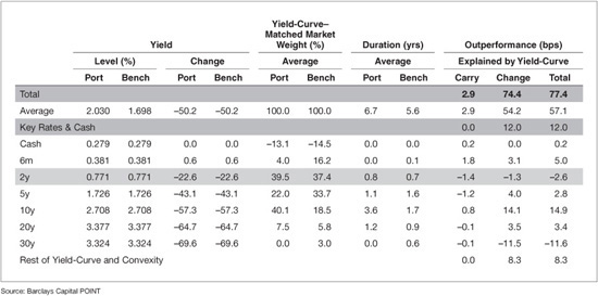
To illustrate how this can be done we will focus on curve carry. The average yield of the portfolio and the benchmark are calculated as the yield of the corresponding yield-curve–matching portfolios. Since the portfolio is longer than the benchmark (as indicated by its higher duration) in an upward sloping yield-curve, its average yield is higher than the benchmark (2.030% versus 1.698%). The corresponding average yield-curve carry contribution can be approximated¹³ using Eq. (70–7) as the excess yield of the portfolio times the elapsed time of one month, (2.030% – 1.698%) × (1/12) = +2.8 bp, close to the +2.9 bp shown. The additional contributions of key-rate points can be estimated using Eq. (70–8). For example, the 2-year point contributes approximately [39.5% × (0.771% – 2.030%) – 37.4% × (0.771% – 1.698%)] × (1/12) = –1.3 bp, close to the –1.4 bp shown.

Outperformance Due to Implied Volatility Exposure

For fixed income securities with optionality, pricing models are typically calibrated to reflect the Black swaption implied volatility surface prevailing in the market. Therefore, changes in implied volatility create returns on the embedded option that must be attributed correctly in performance attribution. Similar to how the contribution of yield-curve changes are measured, both scenario- and analytics-based calculations are used to break down the contribution of implied volatility changes to outperformance. The outperformance due to exposure to implied volatility is typically calculated in terms of volatility decay, parallel shift of the implied volatility surface, and surface reshaping.

Volatility Decay

Volatility decay captures the change in option value due to the lapse of time. The return from volatility decay is difficult to capture exactly, as it requires resimulating interest rate paths and pricing securities using two separate time variables (one for diffusion and the other for discounting). However, volatility decay return can be approximated by subtracting all other components of the total time return, such as yield-curve and spread carry. Outperformance due to volatility decay is the difference between the weighted average volatility decay return of the portfolio and the benchmark.

Implied Volatility Change

The outperformance due to implied volatility change is a result of the difference in volatility exposures of the portfolio and the benchmark and the change in the implied volatility surface. The exposure to parallel shift is measured by Vega, and the parallel shift return is equal to Vega multiplied by the average implied volatility change over the entire surface. The implied volatility surface reshaping return, as well as additional terms that represent other parameters entering the fitting of the implied volatility surface can be calculated as the scenario-based total implied volatility return minus the return from the parallel shift.

Exhibit 70–11 shows a sample implied volatility report¹⁴ produced by the Barclays Capital HPA model. Volatility outperformance is broken down into the contributions of the major asset classes in the portfolio and benchmark.

EXHIBIT 70–11
Implied Volatility Report

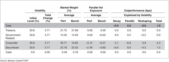
The report contains the initial implied volatility level and its change over the attribution period for each asset class.¹⁵ In this example, implied volatility exposure occurs only in the government-related, corporate, and securitized sectors. The ability of an issuer to call a bond and the prepayment option of mortgage-backed securities give issuers of such bonds optionality, therefore long exposure to implied volatility. Conversely, holders of such bonds are short volatility, as the negative exposure numbers indicate. By being long the corporate and short the securitized sector, the portfolio is implicitly underweighted volatility in the corporate sector and overweighted volatility in the securitized. Since on average implied volatilities increased 5.71% during this month, the corporate sector contributes negatively to parallel volatility outperformance (–0.6 bp), and the securitized sector contributes positively (+6.6 bp). Overall, the portfolio is long volatility since the volatility exposure of the securitized sector is much bigger than that of the corporate and government-related sectors. The total parallel volatility change outperformance contribution is +6.2 bp. The total contribution of changes in the implied volatility surface is calculated from the return splits scenarios, as described above. From that, the surface reshaping (net of the parallel shift) contribution as well as the effects of other parameters and factor of the volatility model are calculated as –3.8 bp. Finally, a net long volatility portfolio will suffer loss of return because of volatility decay. In this case, it has been calculated to be –0.5 bp. Putting it all together, the total contribution of implied volatility to the outperformance of the dollar portfolio is calculated to be +1.9 bp.

FULLY ANALYTICAL MODEL

The Fully Analytical model offers the flexibility to match the increasing diversity in portfolio management structures. It takes full advantage of the return splits by isolating returns from each factor individually. The model can accommodate either bottom-up aggregation or top-down decomposition, depending on how the factor exposures are managed in the portfolio. It is suitable for portfolios with multiple asset classes, as they often have exposures to different market risk factors. For example, consider a portfolio consisting of corporate bonds, mortgage-backed securities and inflation-linked bonds. While all of these securities are exposed to changes in interest rates and possibly implied volatility, mortgage securities have additional exposure to prepayment risk and mortgage spreads, and inflation-linked securities have additional exposure to their reference inflation indices. Similar to how the yield-curve risk is managed, managers of mortgage and inflation-linked securities tend to manage these additional risk factors separately. The ability to break down outperformance due to specific factor exposure can be very valuable to the managers for explaining the impact of their portfolio decisions.

Furthermore, the Fully Analytical model allows portfolio managers to use measures other than market value as allocation weight. This is particularly useful for managers who allocate their capital to various sectors based on risk exposures rather than market values. For instance, a manager taking views on sector spread movement may think of over/underweight in terms of option-adjusted spread duration (OASD). In the credit space, the concept of duration-times-spread (DTS) has been gaining traction in recent years as an alternative measure of spread risk exposure.¹⁶ As a result, credit portfolio managers may prefer to use OASD or DTS as allocation weight in performance attribution.

For illustrative purposes here, we will use the Fully Analytical model with the following choices: Yield-curve and implied volatility are considered common factors and their outperformance contribution is explained using bottom-up aggregation as previously described. The outperformance from mortgage and inflation factors as well as residuals are also explained using bottom-up aggregation and the details of their decomposition is described in the following sections. These factors are calculated per security and can be aggregated to buckets of the selected partition. Outperformance from spread is calculated in a top-down fashion using analytics-based exposure weights for spread change outperformance but market value weights for spread carry outperformance, as described in detail below.

Outperformance Due to Spread

Outperformance from spread is explained using top-down decomposition into asset allocation and security selection per user-defined hierarchical partition or sector. All three components of spread outperformance (carry, spread duration, and spread convexity) are decomposed separately using the top-down decomposition algorithm. Spread carry outperformance is decomposed by applying the absolute allocation algorithm using market value weights and carry returns. We consider two different methods for the decomposition of the spread change outperformance: top-level and sector-level.

Top-Level Spread Model

The top-level spread model assumes that there is a decision to over/underweight the spread duration exposure of the portfolio against the benchmark at the portfolio level (top level). Subsequent decisions to allocate spread duration exposure to various sectors are made relative to the portfolio spread duration. This implies that allocation weight is measured by the ratio of the spread duration contribution of each sector (w_sOASD_s) over the portfolio spread duration. In other words, we apply the relative allocation method of the top-down algorithm of the Chapter 69 using α_k ← OASD, α_{k,s ← ws OASDs, fk,s ← − ΔOAS^B} as hurdle rate.

Here, the Top-Level Exposure term has been renamed Spread Duration Mismatch.

Sector-Level Spread Model

In contrast to the top-level model, the sector-level model assumes no such spread duration decision at the portfolio level. Instead, each asset allocation decision is made without any top-level restriction. In this case, the appropriate allocation weight is the absolute, rather than relative, spread duration contribution. Furthermore, the hurdle rate is set to zero, as sector views are expressed on the absolute (rather than relative) changes in sector spreads. In other words, the absolute top-down decomposition is applied using α_k,s ← w_s OASD_s and f_k,s ← −ΔOAS_s.

Exhibit 70–12 shows the USD Local Management outperformance decomposition of the US Dollar portfolio discussed earlier in this chapter using the Fully Analytical model with either top-level or sector-level spread duration management. We assume two-level allocation of spread exposure, first to major asset classes and then to subsectors of each asset class. In both models a new category, Mortgage,¹⁷ has appeared and is responsible for –8.2 bp of outperformance. In both models, the security selection contribution is +9.3 bp. The difference comes from the treatment of spread duration exposure. The top-level model treats it as a portfolio-level decision (essentially a common return factor) contributing –1.8 bp of outperformance under the label Spread Duration Mismatch, while asset allocation is listed as +5.0 bp. The sector-level model makes spread duration exposure part of the allocation decision and essentially combines the two terms, reporting asset allocation of +3.2 bp.

EXHIBIT 70–12
Outperformance Breakdown Using the Fully Analytical Model

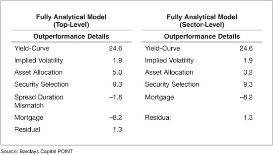
Exhibit 70–13 contains the Asset Allocation report to major asset classes (first level of allocation) using the sector-level model. Outperformance from asset allocation and security selection from each partition bucket is displayed, along with other useful information such as OAS and the changes in OAS, OASD, OASC, and market value weights.

EXHIBIT 70–13
Asset Allocation Report for the Sector-Level Fully Analytical Model

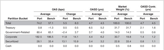
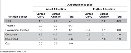
The asset classes with the biggest contribution to spread change asset allocation outperformance are securitized with +4.4 bp and corporate with –1.7 bp. These numbers can be explained as follows. The securitized sector has an underweight of –0.3 years in terms of spread duration (0.8 years versus 1.1 years as seen in the top panel), while benchmark spreads in this sector widened 15.9 bp. Note that since we use the sector-level model, the hurdle rate is zero; therefore, we do not need to compare the spread widening of each sector with that of the benchmark. The approximate calculation estimates the contribution as –0.3 × –15.9 = +4.8 bp, relatively close to the +4.4 bp shown.

Spread carry contributes +1.5 bp to asset allocation, coming mostly from the corporate sector, which has high spread (+186.5 bp versus +57.1 bp for the benchmark) and is market value overweighted (30.7% versus 19.8%). The approximate calculation is (30.7% – 19.8%) × (186.5 – 57.1) × (1/12) = +1.2 bp. Columns for further allocation¹⁸ representing the contribution of spread exposure allocation to subsectors are also included.

Exhibit 70–13 also provides information to confirm the USD spread duration mismatch term from the top-level model (Exhibit 70–12, left panel). Indeed, the portfolio is slightly longer than the benchmark in terms of spread duration (4.7 versus 4.5 years), and benchmark spreads widened by 8.3 bp on average. Multiplying the spread overweight by the negative of the benchmark spread change yields +0.2 × (–8.3) = –1.7 bp close to the –1.8 bp shown in Exhibit 70–12.

Mortgage Factors

The present value of mortgage-related securities depends on additional factors such as prepayments and mortgage rates. Some common additional factors are described below.

Prepayment Surprise Outperformance

Securities involving prepayments are priced using model predictions of future cash flows. Over a month, the realized prepayment rate is generally different from the one predicted by the model. The difference gives rise to a return component that is not captured by analytics; this return can be computed separately as Prepayment Surprise return. In the Barclays Capital Global Aggregate G4 index which is the benchmark in this example, prepayments are recognized on the first of the month based on a predicted rate (which, if different from the model-predicted one, will generate surprise return). Over the course of the month, the actual prepayment rate can be more accurately predicted and used to adjust the returns, leading to more days where the surprise return is non-zero. Once the actual rate is known and returns are adjusted to reflect it, no more surprise return for that particular month will occur. Note that portfolio accounting conventions with respect to recognizing realized prepayments may vary. If they are different from the benchmark conventions, the attribution system will report prepayment surprise outperformance that is not economic but accounting in nature.

Mortgage Spread Change Return

A common factor that affects the cash flows of all mortgage securities is the difference between the model-implied mortgage rate and the actual mortgage rate observed in the market. This difference is called the mortgage spread and the price sensitivity of a security to this spread is the mortgage spread duration. The return due to mortgage spread change is usually estimated with a first order approximation as the product of the mortgage spread duration and the negative of the change in the mortgage spread, i.e., –MtgRtDur · ΔMtgSpread. The outperformance is the difference between the weighted average mortgage spread return of the portfolio and the benchmark.

Other Mortgage Factors

A number of other parameters such as home price appreciation projections and swap spreads may also be used in mortgage pricing models. In the scenario-based return splits, all such parameters are accounted for in Other Market Return scenario. For mortgage securities, the difference between the other market return and the mortgage spread return captures the return from factors for which no analytics are available. If this difference is significant, it is an indication that additional analytics are required to better understand the sources of risk and performance of mortgage securities under the particular valuation model.

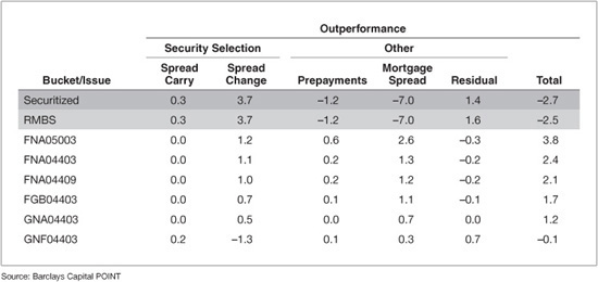
Exhibit 70–14 displays a portion of a detailed position-level outperformance contribution report for the US Dollar portfolio discussed earlier in this chapter. The contribution of each position is broken down per factor. Outperformance components that are allocated in a top-down fashion such as spread carry and spread change are listed under “Security Selection.” Components aggregated in a bottom-up fashion such as mortgage factors and residual are listed under “Other.” Exhibit 70–14 is focused on the securitized sector, which is solely responsible for the –8.2 bp of underperformance attributable to mortgage factors. This report can be very useful to help managers drill down to the position level and understand the drivers of outperformance per individual factor.

EXHIBIT 70–14
Position-Level Report Using the Fully Analytical Model

Inflation Factors

Inflation-linked securities have cash flows linked to a specified price index. For example, the principal and interest payment of U.S. Government Inflation-Linked bonds (TIPS) are linked to the Consumer Price Index for All Urban Consumers (CPI-U), non–seasonally adjusted. The value and the return of inflation-linked securities depend on realized inflation as well as on expectations of future inflation during the lifetime of the security.

The analysis of the risk and performance of inflation-linked securities is subject to debate. One school of thought prefers to treat them as independent of nominal interest rates and express risk and performance as a function of real rates (nominal rates minus inflation expectations). In this type of analysis, the return of inflation-linked securities comes from changes of real rates, as well as time return, which is a combination of real rate carry and realized inflation accretion.

Another school of thought prefers to decompose real rates into the difference of nominal interest rates and inflation expectations such that nominal interest rate risk and contribution to outperformance is accounted consistently across all types of bonds. The numbers shown below are calculated following the latter approach.¹⁹ Inflation expectations are captured by a negative discounting spread (similar to OAS), which is called inflation spread. The return of inflation-linked securities is explained by changes in nominal interest rates and inflation spreads. The time return is captured by the nominal interest rate carry reduced by the negative inflation spread carry and increased by realized inflation accretion. Since realized inflation is announced only once a month, an assumption about the projected inflation of the current month is required to ensure smooth daily inflation accretion. When realized inflation is announced, it is generally different from projected inflation, producing a return that cannot be otherwise accounted for. This kind of return of inflation-linked securities is called inflation surprise and is accounted separately. Inflation surprise return is also present when current month inflation projections change.

Exhibit 70–15 shows the Fully Analytical model’s security return splits for the Barclays Capital Inflation Linked US TIPS index for the period from July 16, 2010 to August 13, 2010. These dates correspond to the CPI-U announcement dates for the index level as of the end of June and July, respectively; therefore, the index should show a realized inflation return equal to the rate of inflation realized during July (but only becoming known on August 13).

EXHIBIT 70–15
Return Splits of Inflation-Linked Securities

The total return of the index was +169.9 bp, with the majority coming from nominal interest rates exposure (+27.7 bp carry and +184.6 bp of yield-curve change). Inflation related return was negative at –40.6 bp, most of it coming from falling inflation expectations (captured under inflation spread change as –29.7 bp). Inflation accretion during July was –3.0 bp, indicating that at the beginning of the month, the market actually expected a small amount of deflation at an annualized rate of –0.03% × 12 = –0.36%. The positive inflation surprise of +5.3 bp indicates that the realized inflation was actually positive, although quite low. The total realized inflation return is +2.3 bp, the sum of inflation accretion (at the market expected rate) and inflation surprise. From that, July realized annualized inflation can be calculated to be approximately +0.023% × 12 = +0.28%. Indeed, the CPI reading for June was 217.965 and the one for July 218.011, implying an inflation rate for July of 218.011/217.965 –1= 2.11 bp or +0.25%. The inflation spread carry term of –13.1 bp reduces the yield-curve carry of +27.7 bp that was credited to the index due to exposure to nominal rates. The difference of the two can be thought of as the carry earned by the index due to exposure to real rates, i.e., nominal rates reduced by inflation expectations.

Another interesting thing to note is that inflation expectations did not fall uniformly across all maturities. Indeed, short bonds exhibited positive inflation spread return, indicating increasing inflation expectations over the next three years or so. This is also the case for very long bonds, with the 30 year bond showing increasing inflation expectations. Inflation expectations fell only for bonds with maturities between 3.5 and 20 years. This indicates that inflation portfolio managers need to pay more attention to the term structure of expected inflation exposure and use more detailed analytics that provide partial sensitivities to the inflation term structure.

SELECTING AN APPROPRIATE ATTRIBUTION MODEL

From the above discussion, it should be clear that many variants of attribution models exist and that a portfolio manager must choose one that best corresponds to the decision structure during portfolio management. The results from several models applied to the U.S. dollar–denominated portion of the portfolio/benchmark from Chapter 69 are summarized in Exhibit 70–16. All models assume two-level asset allocation, first to major asset classes and then to subsectors of each asset class.

EXHIBIT 70–16
Outperformance Contributions Using Various Models

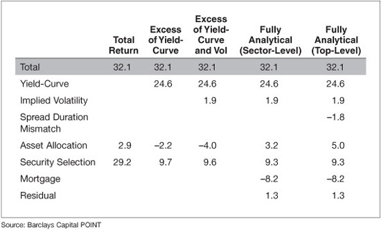
Essentially, models differ with respect to what factors of return are managed at the portfolio level via allocations of appropriate exposures (factor-based management) and which component of return is managed via allocation to sectors and security selection within each sector (sector-based management).

Each successive model brings one additional common factor. The Excess of Yield-Curve model introduces yield-curve exposure as a common factor; the Excess of Yield-Curve and Implied Volatility model introduces implied volatilities; the Fully Analytical model with sector-level allocation of spread exposure introduces all other factors for which there exist explanatory analytics (mortgage factors only, in this particular portfolio) as well as residual; and the Fully Analytical model with top-level allocation of spread exposure introduces top-level spread duration as a common factor.

Flexibility is a very important feature of attribution algorithms. Portfolio management styles differ, and an attribution platform must have sufficient richness so that a model representing each management style can be chosen. In addition, running multiple versions of the performance attribution algorithm may help portfolio managers reveal exposures that they have been implicitly taking and help them improve their management process.

KEY POINTS

• The total return of a security can be broken down to the contributions of various risk factors such as yield curve, volatility, spread, mortgage, and inflation—based on the variables used in the pricing model for that security type.

• Various models can be applied to allocate these components of return in different ways to correspond to the management structure of a portfolio.

• The Total Return Model considers all return as a single allocated factor and divides the difference in performance versus a benchmark into allocation to sectors and sector performance using market value weightings.

• The Excess Return Model extracts common factors, such as yield-curve and volatility, and allocates outperformance from excess return using a top-down algorithm into asset allocation and security selection. Relative performance from common factors is determined using bottom-up aggregation.

• The Fully Analytical model allows any return split component to be extracted as a common factor for bottom-up aggregation. Alternative weights, such as spread duration, can be used in allocation calculations to provide a risk-weighted view.

• It is most effective to choose a primary performance attribution model that matches the management structure of the portfolio. This provides a more effective evaluation of the performance due to exposure to the factors used in the decision making process.