CHAPTER
SEVENTY-ONE
ADVANCED TOPICS IN PERFORMANCE ATTRIBUTION

ANTHONY LAZANAS, PH.D.

Managing Director
Barclays Capital

ANTÓNIO BALDAQUE DA SILVA, PH.D.

Director
Barclays Capital

CHRIS STURHAHN

Vice President
Barclays Capital

ERIC P. WILSON

Vice President
Barclays Capital

PAM ZHONG, CFA

Vice President
Barclays Capital

The principles of performance attribution are outlined in Chapter 69 and a detailed attribution analysis for fixed income portfolios is discussed in Chapter 70. This chapter explores topics that more complex portfolios or analysis may encounter in practice. In particular, we start looking at the attribution exercise in a multicurrency context. Given the fact that the majority of multicurrency portfolios have some type of foreign exchange (FX) hedging overlay, being able to accurately separate the performance due to active FX positions from that due to hedging is a complex but important exercise. Another important topic discussed in this chapter concerns the treatment of returns and outperformance due to the use of derivatives or leverage in the portfolio. Their presence may change the nature of the basis used to define returns, so we discuss in more detail how to change the analysis in order to maintain the integrity of the performance attribution. This chapter finishes with the discussion of other practical considerations that performance attribution exercises often encounter. These include issues such as multi-period compounding, transaction handling, and missing or incorrect input data.

MULTICURRENCY ATTRIBUTION

In Chapter 70, we used performance attribution to examine the portfolio at the local market level, that is, associated with a particular currency market. Multicurrency portfolios add an additional layer of complexity to the portfolio management structure. For instance, there may be decisions made at the global level to determine capital allocation across different local markets or the FX exposures to those markets. In this section, we describe in more detail how one can decompose total global outperformance in terms of FX allocation, local market allocation and local market management.

To study the FX component of the portfolio’s return, we need to define first the base currency of analysis, the currency in which we define the portfolio’s return. Note that by definition, securities denominated in the base currency do not have FX exposure or return.

FX Return Splitting

Since most portfolio managers prefer to manage FX risk separately from all other risk exposures, the first step in return splitting of non-base-currency-denominated securities is to separate the FX component of return from the local component of return. The base currency total return of security i (^bR_i) can be expressed in terms of its local currency return (R_i) and the spot FX return of the currency in which the security is denominated, F_i.¹

Here, we assume that all positions with cash flows or dependencies on interest rates in multiple currencies (such as FX swaps, FX forwards) have been decomposed into legs that have exposure only to the market parameters of a single currency. Note the presence of a cross-term that is the product of the FX return and the local currency return. This can be accounted separately, but in most cases it is combined with the FX return under the assumption that the FX return is typically much larger than local currency returns. While this is generally true for fixed income securities, it may not be true for portfolios that invest in asset classes with higher volatility, such as equities or commodities.

To separate the performance due to FX exposures from the performance due to local management, we need to include the cash deposit return of each currency in the FX return.² Indeed, a cash investment in any foreign currency will earn the FX return plus the local cash deposit return over the attribution period, , without incurring any local risk.

The total return of the portfolio can then be written as the sum of returns from “local markets” that correspond to the first allocation layer of a multicurrency portfolio. Although single-currency markets provide the natural breakdown for FX returns, there is no reason to impose the same breakdown for local returns. In fact many managers allocate local return exposure to markets based on geography, asset class, or industry, rather than currency. We will denote the local return allocation markets with m and we will generally assume that they are not necessarily single-currency markets. Single-currency markets will be denoted with c and will be used for the allocation of the FX component of return, as well as the cross term.

The three terms in Eq. (71–3) correspond to FX, FX/local cross-term, and local returns, respectively. Here, and represent the “base-currency portfolio market value weights,” i.e., the market value of positions in currency c or market m over the market value of the portfolio, both expressed in base currency units. Note that within single-currency markets the cash deposit rate return and the FX return are the same for all securities and therefore the same for the portfolio and the benchmark. However for a generic market m that may span several currencies, the cash deposit rate return is defined as the weighted average return over all market securities. Since the composition of the market generally differs across portfolios and benchmarks we need to use the designation P to identify a specific portfolio.

FX Hedging

FX hedging—the overlay of FX derivatives with the intent to change the FX exposure profile of a portfolio without affecting its local markets exposures—is a common practice in multicurrency portfolios. It enables managers to disentangle the portfolio construction process between the FX experts and the local market managers. The most common instruments used for hedging are FX forwards, typically with short tenors (e.g., one month) and rolled regularly. Longer tenors are sometimes used to reduce rolling costs.

Despite the intent to leave the local exposures unchanged, in practice FX hedging instruments have side effects that must be accounted for in a complete attribution framework. In what follows we detail two such effects.

Exposure to Local Interest Rates

Ideal FX hedges earn the cash rate in each currency and have zero interest rate duration. In practice, FX hedging instruments do have exposure to the short end of local interest rate curves. This effect is highlighted during market crises, when short rates exhibit significant volatility. Typically, this return is considered part of the hedging return, as it comes from an unintended exposure to local rates through the instruments used to hedge the portfolio and is not part of the local rates strategy decisions.

Cash Balance Effect

As FX rates fluctuate, the mark-to-market of FX forwards becomes nonzero, essentially representing a cash balance (positive or negative). Unless such cash balance is reinvested regularly, it represents an unintended allocation to cash (which is equivalent to leveraging if the balance is negative). This effect can be significant and needs to be highlighted in performance attribution. To that end, one possible solution is to capture this effect explicitly as the difference of the actual portfolio return minus the hypothetical return that would be achieved if the FX hedges cash balance were reinvested daily in the portfolio. Similar to the exposures to local rates, this effect should also be reported as part of the hedging return.

Once these side effects have been accounted for, the effect of FX hedges is restricted to the FX component of the total return and the cross-term; the local component of return remains unchanged.

Outperformance from FX Allocation and Hedging

FX outperformance is defined as the part of total outperformance that is due to fluctuations of the exchange-rates between the base currency and all non-base currencies present in the portfolio or the benchmark. The first two terms of Eq. (71–3), pure FX and the FX/local cross-term, contribute to FX outperformance. We look at them separately in what follows.

Let’s denote the effective portfolio exposure to each spot FX rate after hedging with and the benchmark one with Then, we can represent the pure FX outperformance contribution to the portfolio outperformance as follows:

We can now apply the relative allocation model of the top-down decomposition algorithm described in Chapter 69 to get the hedged FX allocation as:

To derive Eq. (71–4), we specifically set the following variables using the notation from Chapter 69: and . The allocation in Eq. (71–4) is typically used to measure pure FX allocation. However, a similar decomposition can be made to the FX outperformance without the hedges. The un-hedged FX allocation would be:

Let’s now discuss the FX-local cross-term return. For simplicity, let’s focus only on the portfolio and split it into the original portfolio (P, with weights w) and the portfolio of hedges (H, with weights w–h). As per Eq. (71–3), we know that the portfolio cross-term return is . However, the hedge portfolio H pays the deposit rate in each currency. Therefore, the net return for the hedged portfolio (P + H) is:

We can therefore see that hedges do contribute to the cross-term between FX and local returns. The contribution of the FX-local cross-term return to the outperformance of a portfolio versus a benchmark is calculated as:

Since this term is the product of two returns, its size is usually smaller than either of the two. However over time, the contributions of the cross-term can accumulate (similar to a convexity term) and become significant relative to the local and FX returns. Moreover, the FX cross-term can be a significant component of total return when FX and local returns have opposite signs and similar magnitudes. For example, if FX return is +5% and local return is –4%, the total return is 5% – 4% + 5% × –4% = 0.80%. Without the cross-term the total return would have been 1.00%, so the cross-term of –0.20% reduces total return by 25%. In the extreme, if the two returns are opposite but equal in magnitude, the entire total return is due to the cross-term. While in the majority of the cases the FX/local cross-term is insignificant, it is preferable to account for it explicitly.

In addition to the first two terms of Eq. (71–3) we just explored, the local return and market value effects of the hedging instruments, as well as their trading returns, should be accounted for separately. This allows us to separate any returns from the hedging instruments from the local returns and outperformance that we explore in the next stage of attribution.

Outperformance from Allocation to Local Markets

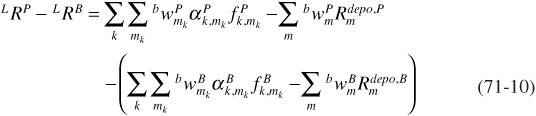
After the contributions of FX exposure and hedging are taken out, the remaining outperformance is given by:

There are many different ways to decompose this outperformance into the contributions of the various decision-makers. The most straightforward is to assume that the first decision layer is the allocation of market value exposure to various local markets. After this, each local market is managed separately versus a corresponding benchmark. We can apply the top-down decomposition algorithm from Chapter 69 to define the local market allocation outperformance as:

And the local market management outperformance as:

Specifically, we use the following notation from Chapter 69 to construct the equations above . Note that this breakdown is equivalent to the Total Return model presented in Chapter 70.

If each local market contains securities denominated in the same currency then Eq. (71–9) is simplified to . The local outperformance within each currency can then be decomposed using the general methodology and any of the models described in Chapter 70. If on the other hand local markets span across currencies, then only the Total Return Model (see Chapter 70) is directly applicable for the analysis of local market management outperformance. The use of models that require a reference interest-rate curve for the analysis is not straightforward.

Factor-Based Local Markets Allocation

Market value-weighted allocation to markets hides many of the complexities of the decision process of investing across markets. Indeed, allocation of exposure to local markets consists of the aggregation of exposure to each risk factor that drives market returns, such as yield-curve, implied volatility, spreads, and so forth. To better quantify how much risk is taken in a particular local market, we can describe the allocation decision using the appropriate exposure to each risk factor, e.g., interest rate duration for yield-curve, Vega for implied volatility and spread duration for spreads, etc.

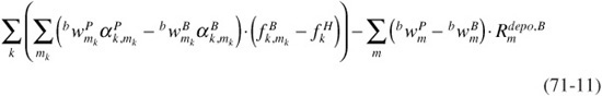
Following the methodology described in Chapter 69, we can rewrite Eq. (71–7) by decomposing local returns into the contributions of risk factors as follows:

As implied by the notation m_k, each factor may use a different set of local markets. We can now separate local outperformance into allocation, management and leverage using different weights for each factor. Specifically, the outperformance due to allocation is:

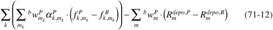
While the one due to management is:

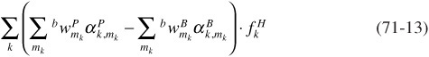
Finally, the top-level allocation, or leverage, can be represented as:

Example: Curve Allocation to Local Markets

As an example of the decomposition we just described, consider a portfolio manager that centrally manages the global interest-rate positioning of the portfolio. In this context, we can use the above methodology to separate the local performance of a portfolio into a global curve allocation and excess (of global curve) outperformance. The portfolio manager can use key rate durations to control her exposure to the former and market value weight to control exposure to the latter. We will select the local markets for the decomposition of global interest rates outperformance in a way that each market c corresponds to a unique interest-rate curve. Most of the time this decomposition is equivalent to single currency markets decomposition, yet occasionally this is not the case. For example, it might be preferable to use individual country government curves when analyzing a portfolio of euro-denominated bonds. This methodology allows us to answer successively:

• What was the contribution of the global duration position of the entire portfolio (Global Duration Mismatch)?

• What was the contribution of taking interest rate exposure (sovereign exposure) outside of our reference currency (Local Curve Advantage)?

• What was the contribution of taking other risk exposure in each currency (Excess of Curve Allocation)?

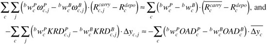
In this example, we will further separate the curve return into two components, a curve carry and a curve change return. To account for curve carry in a way that is consistent with Eq. (71–7), we subtract the deposit return from the outperformance of curve carry. The carry exposure to each individual key-rate point i in each curve c is constructed using the curve-matching portfolio (CMP) weights ω_c,j as described in Chapter 70. The idea behind the CMP is to represent each bond in the portfolio or benchmark as a portfolio of “par bonds” whose curve carry is easy to compute analytically. We can then calculate the carry associated with the portfolio or benchmark using the carry of the corresponding CMP. Let us also denote the curve carry return from each individual key-rate point with . From Eqs. (71–11) to (71–13), using the transformations and setting the hurdle rate equal to the excess carry return of a reference currency (typically the base currency of the analysis) , we get the following decomposition.

The local curve carry allocation is given by

The local curve carry management by

And the global curve carry over deposit as

Note that since c represents a single interest rate curve, the carry return at each key-rate point and the deposit rate return is uniform across all securities and therefore the same for the portfolio or the benchmark. In this case the curve carry management is zero by construction. Further, if we do not use a reference curve, then the global curve carry term also becomes zero and the global curve carry outperformance is simply broken down per curve and key-rate point as follows:

We now turn to the second component of the curve return, the curve change return. The outperformance due to curve change is decomposed similarly using key-rate durations as allocation weights and the negative of the key-rate yield change as return, i.e., , and

Under this setting the local yield-curve change allocation is

And the local yield-curve change management is

Finally, the global duration mismatch is

Once again, within a specific curve interest rate changes are the same for all securities and therefore for the portfolio and the benchmark. This causes the management term to be zero. In addition, if no reference curve is specified, then the global duration mismatch becomes zero as well and the global curve change outperformance is simply broken down per curve and key-rate point as follows:

Once outperformance from interest rate curve exposures has been accounted for, the remaining return, i.e., the return in excess of FX and curve return can be explained using a different set of local markets using the same methodology discussed above in the “Outperformance from Allocation to Local Markets” section.

Global Curve Allocation in Practice

To illustrate the concepts just developed, let’s consider the following example. A U.S. dollar-denominated portfolio is managed against the Barclays Capital Global G4 Treasury Index, an index consisting of government bonds from four currencies, U.S. dollar, euro, Japanese yen and British pound. The manager is allowed to make the portfolio deviate from the index in order to express views that in her opinion will produce superior returns. In this case, the manager believes that euro will strengthen versus the U.S. dollar and at the same time U.S. rates will rise while euro rates will fall. She wants no active exposure to the yen market. Finally, to minimize sovereign risk she prefers to concentrate exposure within the euro-zone to the strongest economies in the region.

The portfolio is constructed in line with the above views as follows:

• The portfolio is long euro (against the U.S. dollar, the base currency of the portfolio).

• The portfolio uses 6-month FX forwards selling Japanese yen against the U.S. dollar to bring the portfolio yen exposure in line with that in the benchmark.

• The portfolio is net long interest-rate duration in euro-denominated securities and net short interest-rate duration in U.S. dollar–denominated securities.

• The portfolio overall interest rate duration is neutral against the benchmark.

• In the euro-zone, only bonds from AAA-rated countries are included in the portfolio.

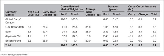
The major portfolio exposures are summarized in Exhibit 71–1.

EXHIBIT 71–1
Portfolio Major Characteristics by Currency

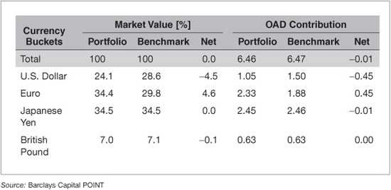
Exhibit 71–2 shows the breakdown of the portfolio outperformance versus the benchmark for a period of one month. The total outperformance is +10.5 bp. It is broken down by currency, with U.S. dollar being the top contributor at +15.5 bp. It is also broken down by type of exposures, where we see that FX positioning contributed +14.3 bp, allocation to local markets (including interest rate exposures) contributed +6.5 bp, while local management within each currency market had a negative contribution of –10.3 bp. As expected, most of the FX Allocation outperformance came from the exposure to the euro (+14.4 bp), indicating that the manager’s view regarding a strengthening euro was correct. The breakdown also shows a small contribution from hedging effects under Japanese yen, +0.1 bp. As discussed previously, the 6-month JPY/USD FX forwards contributed to non-FX return in two ways: (1) They were exposed to the short end of the yen and U.S. dollar yield-curve movements; and (2) over the attribution period they accumulated nonzero market value and therefore created a cash balance effect.

EXHIBIT 71–2
Total Outperformance Breakdown by Currency

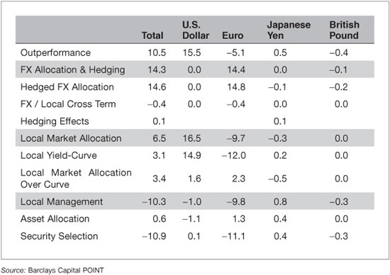
Both effects are captured in the non-zero hedging effects outperformance. The yield-curve allocation outperformance is +3.1 bp, with U.S. and the euro-zone contributing +14.9 bp and –12.0 bp, respectively. From this perspective and for this period, the views the manager had regarding the movements on the yield-curve played well for him regarding the U.S. dollar, but against him regarding the euro. The local market allocation in excess of the yield-curve totals +3.4 bp. Finally, local management pulled back the overall outperformance. Security selection in the eurozone, in particular, contributed –11.1 bp to total outperformance.

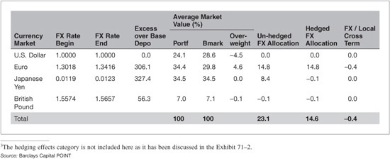
Let us first look into the FX allocation outperformance in detail (Exhibit 71–3). In line with the fund manager’s view, the euro strengthened, producing +306.1 bp of FX plus cash deposit return in excess of the base currency (U.S. dollar) cash deposit return. Since the euro had an average overweight of 4.6% during this period, it contributed +14.8 bp of FX outperformance. This number can be approximated as the product of the average overweight times the excess return of the currency, i.e., 4.6% × 306.1 = +14.1 bp. The number does not tie out exactly with the +14.8 bp outperformance reported in Exhibit 71–3 because in the attribution system it is calculated daily and then compounded taking account of any fluctuations in the exposure. In Exhibit 71–3 one can also observe that FX hedging of the yen exposure cost +8.5 bp of outperformance since the yen also appreciated during this period. However, the reverse could be true should the yen weaken against the U.S. dollar. The return coming from the hedged FX Allocation outperformance for the Japanese yen is close to zero. This shows that the manager was able to implement into the portfolio one of his goals: reduce significantly any volatility related to exposure to the yen.

EXHIBIT 71–3
FX Allocation Outperformance Breakdown by Currency³

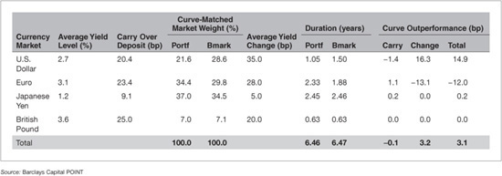
Next, we look more carefully into the global yield-curve outperformance (see Exhibit 71–4). The portfolio curve carry outperformance is almost flat at –0.1 bp. Most of the outperformance comes from portfolio duration positioning. During the period, yields rose for all G4 curves. However, on a relative basis, euro yields rose less than U.S. dollar yields. Without changing the portfolio overall interest rate duration, the portfolio picked up +3.2 bp of outperformance. This was achieved by going short the interest-rate duration in the U.S. (+16.3 bp) while long duration in the euro-zone (–13.1 bp). Overall, the duration decisions played in favor of the manager. Japanese yen and British pound markets contributed little as their durations have been purposely kept neutral to the benchmark.

The outperformance contributions in Exhibit 71–4 have been calculated using Eqs. (71–17) and (71–21) and taking into account the detailed key-rate exposures of the portfolio in each currency. For the purposes of this example we simplify these equations assuming that the portfolio curve exposure is distributed evenly across all key-rate points. In this case the following simplifications can be made:

EXHIBIT 71–4
Global Yield-Curve Allocation Outperformance

Here and represent the average curve carry return and average yield change in each curve.

For example, the average euro yield is about 3.1%, which implies a carryover deposit return⁴ of 23.4 bp over the attribution period (one month). The contribution of the euro market value overweight to curve carry outperformance can be estimated as the market value overweight times the average carry over deposit return, i.e., (34.4% – 29.8%) × 23.4 bp = +1.1 bp. The contribution of the euro duration overweight to curve change outperformance can be estimated as the product of the duration overweight times the negative of the average yield change, i.e., (2.33 – 1.88) × (–28 bp) = –12.6 bp. This is close but not equal to the reported –13.1 bp because of the simplification above as well as the compounding effects over the attribution period. A detailed key-rate level report can be used to gain more insight into the numbers. It is interesting to note that the portfolio market weights in some currencies reported here are different than the ones reported in Exhibit 71–3. In particular, the U.S. dollar weight was 24.1% in Exhibit 71–3 but is now reported as 21.6%; the yen weight was 34.5% but is now reported as 37.0%; the euro and British pound weights are unchanged. This is because the market value of the JPY/USD forwards has been excluded from the local analysis since such positions are considered FX hedges. The contribution of the cash balance effect is captured in the hedging effects category of outperformance as discussed above.

If we analyze the performance by currency as in Exhibit 71–4, we may penalize the fund manager unfairly for the large negative outperformance coming from the Euro exposure. An alternative way to analyze the global curve outperformance is to use a reference curve, as presented in Eqs. (71–14), (71–16), (71–18) and (71–20). This is done in Exhibit 71–5, using the U.S. dollar yield-curve as the reference curve. Although the total curve outperformance remains the same, the breakdown among currencies has changed.

EXHIBIT 71–5
Global Yield-Curve Outperformance with U.S. as Reference Curve

For example, Japanese yen now contributes negatively to the curve carry outperformance. Although the yen has a positive carry over deposit return of +9.1 bp over the month, this return is lower than the U.S. dollar (reference) carry over deposit return of +20.4 bp. Therefore, an overweight in a relatively underperforming currency results in an underperformance. The global carry outperformance can be approximated with the formula

This approximation is always zero since the sum of the weights over all curves of an (unleveraged) portfolio or benchmark is equal to 1. However, since the actual calculation is using exposures at each key-rate point, the exact global carry outperformance may be non-zero.

The euro shows now a positive contribution to the curve change outperformance due to better performance relative to the U.S. curve. Its contribution to curve change outperformance is now estimated as – (2.33 – 1.88) × (28 bp – 35 bp) = +3.2 bp, close to the +3.1 bp reported. As concluded before, the manager decision regarding global curve positioning had an overall positive performance for the portfolio during this period. The U.S. curve—being the reference curve—does not contribute to outperformance. The global duration contribution can be estimated using the formula –(OAD^P – OAD^B)·. , i.e., – (6.46 – 6.47) × 35 bp = +0.3 bp, close to the +0.1 bp reported.

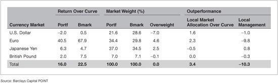
After the yield-curve outperformance has been accounted for, the excess of yield-curve return is split into allocation and management components. Although in general a different set of markets can be used, in this example we will use the same G4 markets used for the curve decomposition. Exhibit 71–6 shows the details of this breakdown. Overall, the allocation of exposure to the four markets has contributed positively (+3.4 bp) with the exposure to the euro market contributing most of it (+2.3 bp). This number can be approximated as the overweight of the euro market times the excess return of the euro market in the benchmark relative to the overall benchmark, i.e., 4.6% × (67.9 bp –22.5 bp) = +2.1 bp. On the other hand, the local management of excess to curve return in the euro market has not been successful, contributing –9.8 bp to outperformance. The approximate calculation yields 34.4% × (40.5 bp – 67.9 bp) = –9.4 bp. This underperformance can be understood by looking at more detailed issuer-level reports as presented in Chapter 70. In this example, it turns out that the lower-rated EU countries experienced much bigger spread tightening during the period. The concentration in the strongest economies in the region may reduce the portfolio long-term risk, but during this particular period contributed to loss of performance.

EXHIBIT 71–6
Excess of Yield-Curve Outperformance

DERIVATIVES AND LEVERAGE

Derivative instruments are widely used across asset classes as both hedges and means to express market views. Their payoffs are tied to changes in the values of underlying securities, and their market values do not generally represent the size of the actual exposure to risk factors. In this section, we discuss how a performance attribution model may handle derivative instruments in order to maintain the intuitive and meaningful nature of the results.

Returns and Basis

Returns of derivative instruments can be difficult to measure. The market value of a contract is typically small (or sometimes zero) compared with its notional exposure, and the standard definition of return—profit/loss (P&L) divided by market value—can result in extremely large (or even infinite) values. For example, the market value of instruments that are marked-to-market daily, such as Treasury futures, is guaranteed to be zero at the end of the day, resulting in a theoretically infinite return. To maintain the notion of return as a P&L per unit of investment, we seek to use a denominator that represents the size of the position in terms of its exposure. We refer to this quantity as the “return basis” or simply “basis.” One should define an appropriate return basis for each derivative type of interest. Usually, the basis is set equal to the notional amount, although in many cases special rules are used to define the basis in a bond-equivalent way.

To complicate the issue of derivatives further, the standard methodology of multi-period return compounding cannot be applied. Consider the following definition of single- and multi-period returns, where PL_t and R_t are the P&L and return over the period (t–1, t). The portfolio return is given by

And the multi-period return is:

By using market value as a basis for the return and compounding it with the above formula, we get an intuitive relationship between the market values at t = 0 and t = T, and the return over the period (0, T).⁵

Changing the basis to a quantity that is not proportional to the market value will annul this property. This is more evident when returns are large. As an exaggerated example, consider a futures contract that is marked to market daily and therefore always has zero market value. A reasonable basis for returns for a position in this contract is the notional amount invested. Suppose the notional amount is $1,000 and that over two days, the contract produces a mark-to-market P&L of –$500 and $1,000, respectively. Using the notional amount as the basis of returns, the returns for the two days are –50% and +100%, respectively. Using the chain rule to compound returns yields zero return over the two days: (1 – 50%)×(1 + 100%) – 1 = 0%. Obviously, this is not consistent with the positive P&L of $500 produced over the two days. Such effects are always present when compounding returns using a basis that is different from the market value of the position; however, their effect is much smaller when the magnitude of returns is small. To avoid such nonintuitive results, one should make appropriate adjustments to the compounding of returns of derivative securities—something out of the scope of this chapter.

Returns for Portfolios and Sectors Containing Derivatives

The return of each individual derivative contract is defined using its basis as described above. However, in typical portfolios, these contracts coexist with cash securities. When we analyze partitions of the portfolio, such as sector or rating, that contain both cash and derivative securities, it is still typical to use market value as the denominator for all returns and weights.⁶ Nevertheless, the presence of the derivatives imposes some changes into the analysis.

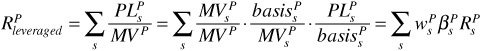
Let’s define the leverage ratio for each security, β_i, to be the basis divided by the market value of the security. Then the leveraged weight of the security is the product of the market value weight and the leverage ratio, w_iβ_i. The return of the portfolio or sector can then be written as the leveraged weighted sum of the deleveraged return of each security:

Although this transformation does not change the return, notice that the leveraged weights are no longer constrained to sum to 1 when derivatives are present in the portfolio.

Therefore, when we seek to explain the contribution of each instrument to the security selection outperformance of each bucket (the last step of the top-down decomposition—see Chapter 69), derivatives give rise to an additional term of outperformance that comes from the implicit leverage they introduce. The example below illustrates this issue.

Example: Leverage from Derivatives and Security Selection Outperformance

Consider a bucket with a single credit security A experiencing excess of curve return of +10%, while the corresponding benchmark bucket has two equally weighted securities, the one in the portfolio A and another one B returning 0%. The total return for that bucket in the benchmark is therefore +5%. Let us also assume that the market value weight of this bucket in the portfolio is 20%; therefore, its contribution to security selection would typically be calculated as 20% × (10% − 5%) = 1.0%. The contribution of security A to security selection is calculated as 20% × (100% − 50%) × (10% − 5%) = 0.5%, and the one of security B is 20% × (0% − 50%) × (0% − 5%) = 0.5%.

Now assume that the portfolio also contained a short protection credit default swap on the issuer of bond A with a return basis equal to the market value of A, essentially doubling the exposure to the issuer of A. Let us assume that the default swap is at-the-money, i.e., its market value is zero, and that it also experiences a return of +10% (using notional as the return basis). Since the market value of the portfolio bucket remains the same but its P&L doubles, the return of the sector is now reported as +20%, and the security selection term becomes 20% × (20% − 5%) = 3.0%. Notice that the market value weight of the bond remains 100% and that the default swap also has a weight of 100% (return basis over market value of the bucket). Bonds A and B contribute to security selection 0.5% exactly as before. The default swap contributes 20% × (100% − 0%) × (10% − 5%) = 1.0%. The contributions of the three securities to security selection sum to 2.0%, leaving 1.0% of security selection unexplained.

This comes from the leverage introduced to the bucket. Indeed, the sum of securities weights in the portfolio is 200%, whereas in the benchmark it is 100%. This causes an outperformance of 20% × (200% −100%) × 5% = 1.0%, completing the decomposition of security selection. This term was introduced as the “top-level exposure” for the excess return model in Chapter 70 (see Eq. (70–6)).

Typically, in the presence of derivatives, this top-level term can be reported as a separate line item for each bucket–bucket leverage, and folded into the security selection term. Alternatively, it can be reported as leverage at the portfolio level.

A General Framework for Leverage

Leverage complicates portfolio returns calculations and comparison to the benchmark. Furthermore, there are different means to achieve leverage, and the decision to employ it can occur at any level of the portfolio management decision structure. For instance, cash borrowing can be used to leverage the entire portfolio, while derivatives can be used to leverage specific sectors. The latter case can be further distinguished into a decision made by an asset allocator or by a sector manager. Below, we outline an analytical way to account for leverage in a consistent framework with the one discussed in Chapter 69.

We expand the concept of leverage ratio as introduced before and apply it to the entire portfolio. We assume that a “funded” market value—generally different from the actual market value—can be defined for the portfolio, partition buckets and individual securities, and serve as the basis for the calculation of unleveraged returns. The ratio of the returns basis to actual market value is the leverage ratio of the portfolio.

We can also recursively break down the portfolio return into the contributions of its various sectors by appropriately defining the leverage ratio of each sector:

Using similar terminology for the benchmark, the total leveraged outperformance can be expressed as a function of leverage ratios and unleveraged returns as:

We will now consider the different ways to break down the total outperformance into contributions from asset allocators and sector managers. It is worthwhile to note that when leverage is allowed, there is no limit to how much exposure managers can allocate to sectors or securities. Consequently, it no longer makes sense to compare sector returns against a hurdle rate (as discussed in Chapter 69) to determine the contribution from asset allocation decisions.

Separate Allocation of Market Weight and Leverage of Each Sector

In this case, each sector is given a market value budget, but sector managers are free to take leverage within their sectors. Separate agents determine the market value allocation and the leverage in each sector. The simple asset allocation/sector management equations can be readily applied in this case. The comparison of sector returns of the portfolio and the benchmark occurs on a leveraged basis. In this case, the outperformance from leverage decisions is embedded in the sector management term. Specifically, the asset allocation would come as

And the sector management as

Allocation of Total Exposure to Sectors

Alternatively, leverage can be determined by the asset allocator instead of the sector managers. In this case, a single agent decides the total exposure⁷ to the unleveraged return of each sector. Once again, the asset allocation/sector management equations can be applied, but we now need to use total exposure instead of market value as the allocation weight. In this case, the outperformance from leverage decisions is embedded in the asset allocation term. The asset allocation is

While the sector management comes as

In general, we can assume that leverage decisions are made at both the portfolio and the sector levels. A top-level manager may determine the total portfolio leverage (relative to the benchmark), and an asset allocator may subsequently determine the total exposure to each sector. Therefore, if total leverage is determined at the portfolio level, then the allocation of total exposure to each sector is constrained by the portfolio leverage decision and must be measured relative to that. Instead of using the absolute total exposure as the allocation weight, we now need to use the relative total exposure (total exposure divided by the portfolio/benchmark leverage). We also need to use a hurdle return, as exposure at the sector level is partially constrained.

In this scenario the outperformance decomposition has some extra terms, as shown below. The asset allocation outperformance can be derived as

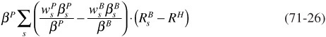
While the sector management comes as

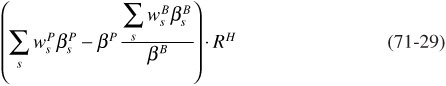
The top-level leverage is

If we do not assume that leverage aggregates linearly, i.e., generally and in order to keep the decomposition complete we need to add an additional term, that we call “diversification.”

If we assume no leverage in the benchmark, the diversification term becomes

Moreover, this term is zero if the leverage is aggregated linearly; that is,

However, there are situations where we may not want the leverage to aggregate linearly. As an example, suppose that betas are defined based on risk. Then, if the different sectors are not perfectly correlated, the beta of the portfolio would tend to be smaller than the sum of the individual sector betas. This is due to the well-known risk diversification effect, hence the name for this term. In this case, the leverage creates a diversification effect with positive returns for our portfolio as long as the hurdle rate return is positive.

Handling leverage is a generalization of the top-down decomposition algorithm described in Chapter 69, where unleveraged returns are the factor returns, leveraged weights are the factor loadings and we assume linear aggregation of leverage (so that the diversification term vanishes). This analysis is also similar to the one regarding the decomposition of the spread related outperformance, described in Chapter 70.

Special Handling of Certain Derivative Types

Often, derivatives are used to manage a specific type of risk exposure and are not meant to participate in the general asset allocation/security selection portfolio management framework. We already encountered this issue earlier in this chapter, while discussing how to handle the role of currency derivatives as FX hedging instruments. A similar situation arises with interest-rate derivatives as instruments of managing interest-rate risk only. In both cases we have to account for the return that is not tied to their primary hedging function and for the implicit cash allocation that occurs when derivative instruments used as hedges acquire market value between rebalancing dates. On the other hand, credit derivatives are typically used along with cash instruments to manage exposures to sectors and issuers; therefore they do participate in asset allocation and security selection. Depending on the portfolio and level of analysis, we may want all these different effects to be captured and reported separately. Below, we discuss in more detail issues arising from the handling of common derivatives and the treatment typically adopted.

Currency Derivatives

FX forwards are typically used as FX hedging instruments. In this case, their return and outperformance contributions should not be allowed to affect the local (excess of FX) outperformance analysis. As discussed previously in this chapter the easiest way to achieve this is to remove them completely from the analysis of non-FX outperformance. However, removing FX hedges from the local analysis introduces two side-effects that have to be explicitly accounted for: (a) The nonFX return of FX hedges must be recorded. Such return can be non-negligible in periods of market crisis or whenever hedges with longer tenors are being used. (b) Since FX hedges are not being rolled daily, they accumulate market value which represents an allocation to cash, if positive, or leverage, if negative. This effect—called earlier as the “FX hedging cash balance effect”—contributes to outperformance and should be appropriately recorded.

Interest Rate Derivatives

Derivatives designed to hedge or gain exposure to interest rate factors are typically overlays onto a portfolio after the core positions are chosen. These instruments, such as government bond futures and interest rate swaps, typically affect the curve return of the portfolio but have little effect on the excess return over yield-curve. Typically, they are used in portfolios that lend themselves to attribution models that treat curve outperformance separately (e.g., the excess return model discussed in Chapter 70). In these models, interest rate derivatives should only contribute to the curve outperformance, which is a common factor, and they should be removed entirely from the decomposition of the allocated factors. Two portfolios identical except for the use of interest rate derivatives should have the same asset allocation and security selection returns.

Similar to currency hedges, the removal of interest rate derivatives from the asset allocation/security selection outperformance analysis introduces a cash-balance effect if the market value of such derivatives is non-zero. Indeed, a positive market value indicates an implicit allocation to cash, whereas a negative market value indicates implicit borrowing and, therefore, leverage. Further, exchange-traded derivative instruments may incur return that cannot be explained by their curve exposures. For example, Treasury futures frequently trade at a spread to their theoretical fair value. Changes in this spread result in return that cannot be explained by interest rate movements. However, this return should be accounted for and reported as a side-effect of interest rate hedging.

Credit Derivatives

In contrast to currency and interest rate derivatives, credit default swaps (CDS), credit index default swaps (CDX or iTraxx), and total return swaps (TRS) are primarily used to manipulate exposure to excess (over curve) return factors. Typically, these instruments are included in the regular asset allocation/security selection decomposition. Single issuer credit default swap instruments have small interest-rate exposure which does contribute to the yield-curve outperformance, but their primary exposure is to the credit factor of the underlying issuer. The performance of credit default swap indices should be explained by exploding them into their single-issuer constituents. The constituents are then included in the asset allocation/security selection decomposition, ensuring that the correct weights and returns are used to reflect the actual exposure to each partition bucket. The basis of returns for credit derivatives is not their market value. As a result, they generate bucket leverage, as discussed previously.

FROM THEORY TO PRACTICE

In order to be of any practical use, a performance attribution system must deal with a significant number of special situations that arise in day-to-day portfolio management. Such issues include missing security prices or analytics, bad prices or analytics, intra-period transactions, settlement conventions, pricing discrepancies between the portfolio and its benchmark, and so on. Below, we discuss some of these issues.

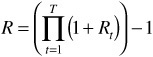
Return and Outperformance Compounding⁸

Multi-period arithmetic total return is compounded by taking the product of the single-period total returns:

As discussed in Chapter 69, a general framework of performance attribution begins with the splitting of a single-period total return into the contributions of various factors, . This leads to the question of how the return splits should be compounded so that the sum of the compounded return splits remains equal to the compounded total return. This is necessary to satisfy the additivity and completeness requirements of attribution.

One way to accomplish this is the following: Let us designate with the multi-period compounded factor return. Setting equal to the single-period factor return, f_k,t, scaled by the compounded portfolio value at the beginning of the period, i.e.,

guarantees the additive decomposition of total multi-period return, i.e., This decomposition algorithm is fairly straightforward and has the properties of additivity and completeness, but what about fairness?

Consider a simple example with two factors and two periods. Let us assume that both factors contribute 20% return, but factor A does so in the first period and has zero return in the second period, while factor B has zero return in the first period and 20% return in the second period. The total portfolio return is therefore (1 + 20%) × (1 + 20%) – 1 = 44%. According to the algorithm above, the contribution of the first factor is not scaled because it occurs in the first period and remains at 20%; the contribution of the second factor is scaled by the portfolio value at the end of the first period (1.20) so it becomes 24%. Although one could argue that the decomposition is unfair—as it favors the second factor which contributed returns after the first factor—the notion that later returns and contributions can be affected by the earlier performance of the portfolio as a whole is generally accepted as a fair practice.

In addition to the total return and return splits compounding, any multi-period attribution algorithm also needs to address the compounding of outperformance. In the context of simple factor-based performance attribution models the above algorithm can be readily applied:

However, in the context of a general attribution model where the categories to which outperformance is decomposed to may depend both on the portfolio and the benchmark (e.g., asset allocation or security selection), such simple decomposition is not possible and more complex algorithms must be used.

Since single-period performance attribution provides a complete, additive and fair decomposition of single-period outperformance, most compounding algorithms seek to define scaling coefficients for each period, such that the sum of the scaled single-period outperformance is equal to the total multi-period outperformance.⁹

Once β_t is determined, it can be used to scale every outperformance component (e.g., yield-curve, asset allocation, security selection, etc.) because of the additivity and completeness properties of single-period performance attribution.

One commonly used approach in practice is the optimized linking coefficient approach.¹⁰ The basic idea behind this approach is to seek coefficients which avoid extreme values under most scenarios. Indeed, if not carefully defined, such coefficients can become zero or attain very high values distorting the outperformance decomposition and making it unfair. The value of β_t in the optimizedlinked method is determined as follows:

Transactions

Return and outperformance calculations require special treatment of transactions. Security transactions which usually settle on a forward basis create “intra-period” returns as well as “unsettled” positions. It is important to recognize intra-period return separately because it does not participate in the decompositions previously discussed. It is also important to make the distinction between settled and unsettled positions because only the settled positions earn carry.

Intra-Day Return

Daily attribution models compound returns and outperformance using end-of-day market-closing prices. However, the models should allow users to enter transactions that occur during the day at the actual transaction prices, which can be quite different from the closing prices of the traded security used to calculate daily returns. This flexibility guarantees that the returns of the portfolio, including trading activities, are captured accurately. The difference between the trade price and the closing price should be captured and reported separately as “Trading” return. Further, the return contribution from intra-day trading activities, which is not captured by the end-of-day portfolio snapshots, must also be accounted for and reported as “Intra-Day Trading” outperformance.

Unsettled Positions

Most security transactions settle on a forward basis; i.e., both cash and the security are exchanged some days in the future. For example, corporate securities transactions settle after three business days (T+3), while most government securities settle after one day (T+1). Certain mortgage-backed securities (TBAs) have special settlement rules as they settle on a specific day each month. A comprehensive attribution model should allow transactions to settle on any forward date.

While buyers of a security are exposed to its clean price fluctuations (market risk) immediately after the transaction, they do not begin earning the coupon return of the security (more accurately, the yield or time return of the security r^carry) until after the settlement date. Instead, they keep earning the yield on the cash (r^cash) that they have promised to pay on the settlement date. Therefore, an unsettled position in a portfolio is earning a return equal to r^cash + r^price, while the same security in an index, always settled, is earning r^yield + r^cash. The return (r^cash – r^yield). Δt, where Δt is the time to settlement, constitutes real outperformance (usually negative) that must be accounted for. Conversely, when the portfolio sells the position, it is earning the security yield (instead of cash) until the sell settlement date, making back any yield lost when the security was bought. These effects should be captured by the outperformance algorithm and reported for each model as carry outperformance.

Handling Inconsistent or Missing Data

Security prices used to compute returns of benchmark indices may be different from what portfolio managers use to mark their positions.¹¹ For any outperformance decomposition to be meaningful, it is important for the price and, hence, the return of the same security to be consistent in both universes. In most cases, managers would want to use their own prices to compute their portfolio returns. In general, we should use the security returns from the portfolio by default. However, since the total return of the benchmark index typically needs to be consistent with the published number, the algorithm should allow for the pricing difference effect to be reported as a separate source of outperformance.

When there are missing prices during the attribution period, the system can either exclude the securities from the analysis entirely or imply prices if that is deemed reasonable. During the period with missing prices, one can use last available analytics and market changes to imply prices so that daily outperformance can be computed. This approach is particularly useful if prices for the beginning and end of the period are available so that the correct return over the attribution period is known.

KEY POINTS

• Multi-currency portfolios add an additional layer of complexity to the portfolio management structure. An attribution algorithm normally needs to decompose the global total outperformance into FX and local market allocations, as well as local management.

• Being able to accurately separate the performance due to active foreign-exchange (FX) positions from that due to the hedging effects is a complex but particularly important task in any multi-currency attribution system.

• Factor-based local market allocation, such as duration-based global curve allocation, quantifies better the risk and return in a particular market than the market-value weighted local markets allocation.

• Derivatives change the nature of the basis used to define returns. They often require special treatment in order to obtain intuitive and meaningful attribution results.

• Return and outperformance compounding is an important task in order to ensure the additivity and completeness properties for any multi-period attribution.

• A complete attribution system should be able to handle intra-day transactions, unsettled positions as well as missing and inconsistent prices.