Ohm's Law Still Works: Constantly Drill the Fundamentals

Ohm's Law

This, I believe, is one of the best-taught principles in school for the budding engineer or technician, and it should be. So why go over it? Well, two reasons come to mind: One, you can't go over the basics too much, and two, though any engineer can quote Ohm's Law by heart, I have often seen it ignored in application.

First, let's state Ohm's Law: Voltage equals current multiplied by resistance; it is shown in Figure 2.1 on the next page.

It is simple, but do you consider that resistance exists in every part of a circuit¹? It is easy to forget that, especially since many simulators do. I think the best way to drive this point home is to recount the way it was driven home to me.

There I was—a lowly engineering student. I was working as a technician or associate engineer (depending on whom you asked). I was arguing with my boss, who had an MSEE degree, but he just wouldn't believe me; neither would my lead engineer (who had a BSEE). I couldn't bring myself to distrust Ohm's Law, even in light of their “superior” knowledge. I'd had less heated debates with rabid dogs. This was the problem: Our department needed to measure the current of a DC motor that could range from 5 A to 15 A at any given time, but our multimeters had a 10 A fuse in the current measuring circuit.

So, using Ohm's Law (which was fresh in my mind, being a student and all), I designed a shunt to measure current. I wanted to get a good reading but disturb the circuit as little as possible, so I chose a 0.1 Ω resistor. I built a box to house it and installed banana-jack plugs to provide an easy interface to a voltmeter. The design looked like the one shown in Figure 2.2

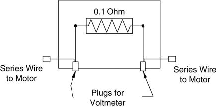
Everyone thought it was a great idea, so I built a couple of boxes and we started using them right away. After a while, however, we noticed that they were not very accurate. Sometimes they would be off by as much as 50 to 60%. No one could figure out why, so I sat down to analyze what I had created.

After a few minutes, I said to myself, “Well, duhhh!” I realized that to make the assembly easy I had soldered the wires from the motor to the banana jacks and then soldered some short 14-gauge jumpers to the shunt resistor. My circuit really looked like the drawing shown in Figure 2.3.

My voltmeter was measuring across a larger resistance value than 0.1ohms. Wire has resistance, too; even a couple of inches of 14-gauge wire has a few hundredths of an ohm. Remembering Ohm's Law:

$V=I*R$ Eq. 2.1

Eq. 2.1

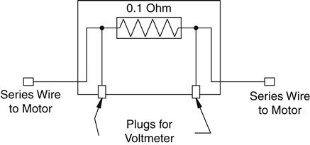
I realized that this means if you increase R, you get more V for the same amount of current, leading to the errors we were seeing. I had made a simple mistake that fortunately was easy to correct. I redesigned the box on paper to look like the drawing in Figure 2.4.

I took this to my boss (the one with the MSEE who could do math in his head that I would only attempt with MathCad and a cold drink). His reaction floored me. He reviewed it with the lead engineer and they came to the conclusion that I was completely wrong. They were talking about things like temperature coefficients and phase shifts in current and RMS and a bunch of other topics that were over my head at the time. Thus began the argument. I explained that two points on a schematic had to be connected by a wire and a wire had resistance. Though it is often ignored, it was significant in this case because the shunt resistor was such a small value.

As they hemmed and hawed over this, I learned that many times it is human nature to ignore what one learned long ago and try to apply more advanced theories just because you know them. Also, all the knowledge in the world isn't worth jack if it is incorrectly applied. I continued to press my point. I must have written Ohm's Law on the white board 50 times by then.

They finally conceded and agreed that the extra wire between the banana jack and the shunt was the cause of the error. That was not the end of the disagreement, though. How in the world was my new design going to fix the problem by simply repositioning the wires? The resistance was still in the circuit, was it not? I wrote down Ohm's Law another 100 times and explained that the current through the meter was very small, making the resistance in the wire insignificant again. My astonishment reached new levels as I observed the human ability to overlook the obvious. The first argument was nothing compared to this one. The fireworks started to really fly then.

What is the moral of this story? Well, Scott Adams, creator of Dilbert, said, “Everyone has moments of stupidity,” as he watched someone fix his “broken” pager by putting in a new battery. I have to agree with him. I rediscover Ohm's Law about every 6 months. Always, always, always check the basics before you start looking for more complicated solutions! My father, a mechanic, tells a story of rewiring an entire car just to find a bad fuse. (It looked okay but didn't check out with a meter.) That was how he learned this lesson. Me, I just participated in 4 hours of the dumbest argument of my career.

How did the argument end? We never came to an agreement, so I went ahead and fixed boxes with the new design anyway (which they spent several weeks proving were working correctly). I didn't say another word but transferred out of that ! as soon as possible. The same design has been in use for over 10 years now, and the documentation notes the need to wire it correctly to avoid inaccurate readings. I didn't write that document, my old boss did. It's kind of funny how we didn't argue about Ohm's Law after that.

The basics are the most important; let me repeat that, the basics are important! Ohm's Law is the most basic principle you will use as an electrical engineer. It is the foundation on which all other rules are based. The fundamental fact is that resistance impedes current flow. This impedance creates a voltage drop across the resistor that is proportional to the amount of current flowing through it. If it helps, you can think of a resistor as a current-to-voltage converter.²

With that important point made, let's consider two other types of impedance that can be found in a circuit. We will get into this in more detail later, but for now consider that inductors and capacitors both can act like resistors, depending on the frequency of the signal. If you take this into account, Ohm's Law still works when applied to these components as well. You could very well rewrite the equation to:

$V=I*Z$ Eq. 2.2

Eq. 2.2

Think of the impedance Z as resistance at a given frequency.³ As we move on to the other basic equations, keep this in mind. Wherever you see resistance in an equation, you can simply replace it with impedance if you consider the frequency of the signal.

One final note: Every wire, trace, component, or material in your circuit has these three components in it: resistance, inductance, and capacitance. Everything has resistance, everything has capacitance, and everything has inductance. The most important question you must ask is, “Is it enough to make a difference?” The fact is, in my own experience, if the shunt resistor had been 100 times larger, that would have made the errors we were seeing 100 times less.⁴ They would have been insignificant in comparison to the measurement we were taking. The impedance equations for capacitors and inductors will help you in a similar way. Consider the frequencies you are operating at and ask yourself, “Is this component making a significant impact on what I am looking at?” By reviewing this significance, you will be able to pinpoint the part of the circuit you are looking for.

The experience I related earlier happened years ago at the beginning of my career, and I said then that I still rediscover Ohm's Law every six months. Time and time again, working through a problem or design, the answer can be found by application of Ohm's Law. So, before you break out all those higher theories trying to solve a problem, first remember: Ohm's Law still works!

The Voltage Divider Rule

Next on our list of basic formulae is the voltage divider rule. Here is the equation and Figure 2.5 shows a schematic of the circuit:

$\mathit{Vo}=\mathit{Vi}\frac{\mathit{Rg}}{\mathit{Rg}+\mathit{Ri}}$ Eq. 2.3

Eq. 2.3

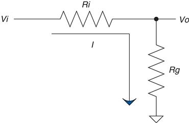
The most common way you will see this is in terms of R1 and R2. I have changed these to Rg (for R ground) and Ri (for R input) to remind myself which one of these goes to ground and which one is in series. If you get them backward, you get the amount of voltage lost across Ri, not the amount at the output (which is the voltage across Rg). If the gain⁵ of this circuit just doesn't seem right, you might have the two values swapped.

You might also notice that the gain of this circuit is never greater than 1. It approaches 1 as Ri goes to 0, and it approaches 1 as Rg gets very large. (Note that as Rg gets larger, the value of Ri becomes less significant.) Since this is the case, it is easy to think of the voltage divider as a circuit that passes a percentage of the voltage through to the output. When you look at this circuit, try to think of it in terms of percentage. For example, if Rg=Ri, only 50% of the voltage would be present on the output. If you want 10% of the signal, you will need a gain of 1/10. So put 1 K in for Rg, and 9 K in for Ri, and, voilà, you have a voltage divider that leaves 10% of the signal at the output.

Did you notice that the ratio of the resistors to each other was 1:9 for a gain of 1/10? This is because the denominator is the sum of the two resistor values. I'll also bet you noticed that if you swap the two resistor values you will get a gain of 9/10, or 90%. This should make intuitive sense to you now if you recognize that, for the same amount of current, the voltage drop across a 9 K Ri will be nine times larger than the voltage drop across a 1 K Rg. In other words, 90% of the voltage is across Ri, whereas 10% of the voltage is across Rg, where your meter measuring Vo is hooked up. The voltage divider is really just an extension of Ohm's Law (go figure), but it is so useful that I've included it as one of the basic equations that you should commit to memory.

Capacitors Impede Changes in Voltage

Let's consider for a moment what might happen to the previous voltage divider circuit if we replace Rg with a capacitor. It is still a voltage divider circuit, is it not? But what is the difference? At this point you should say, “Hey, a cap is just a resistor that's value changes depending on the frequency; wouldn't that make this a voltage divider that depends on frequency?” Well, it does, and this is commonly known as an RC circuit. Let's draw one now, as shown in Figure 2.6.

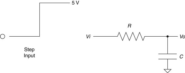
Using your intuitive understanding of resistors and capacitors, let's analyze what is going to happen in this circuit. We'll do this by applying a step input. A step input is by definition a fast change in voltage. The resistor doesn't care about the change in voltage, but the cap does. This fast change in voltage can be thought of as high frequencies,⁶ and how does the cap respond to high frequencies? That's right, it has low impedance. So, now we apply the voltage divider rule. If the impedance of Rg is low (as compared to Ri), the voltage at Vo is low. As frequency drops, the impedance goes up; as the impedance goes up, based on the voltage divider, the output voltage goes up. Where does it all stop?

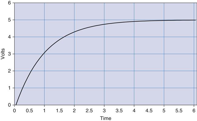
Think about it a moment. Based on what you know about a cap, it resists a change in voltage. A quick change in voltage is what happened initially. After that our step input remained at 5 V, not changing any more. Doesn't it make sense that the cap will eventually charge to 5 V and stay there? This phenomenon is known as the transient response of an RC circuit. The change in voltage on the output of this circuit has a characteristic curve. It is described by this equation:

$\mathit{Vo}=\mathit{Vi}\left(1-e^{-\frac{\tau }{\mathit{rc}}}\right)$ Eq. 2.4

Eq. 2.4

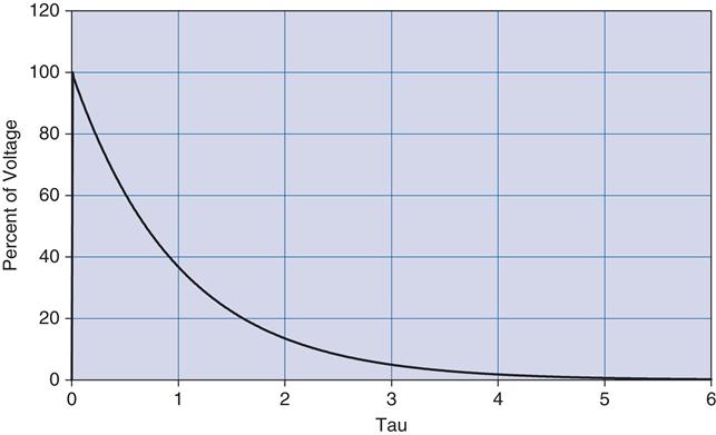
The graph of this output looks like Figure 2.7. The value of R times C in this equation is also known as tau, or the time constant, often referred to by the Greek letter τ.

$\mathrm{RC}=\tau$ Eq. 2.5

Eq. 2.5

For a step input, this curve is always the same for an RC circuit. The only thing that changes is the amount of time it takes to get to the final value. The shape of the curve is always the same, but the time it takes to happen depends on the value of the time constant⁷ tau. You can normalize this curve in terms of the time constant and the final value of the voltage. Let's redraw the curve with multiples of τ along the time axis, as shown in Figure 2.8.

At 1 τ the voltage reaches 63.2%, at 2 τ it is at 86.6%, 3 τ is 95%, by 4 τ it is at 98%, and when you reach 5 τ you are close enough to 100% to consider it so.

This response curve describes a basic and fundamental principle in electronics. Some years ago I started asking potential job candidates to draw this curve after I gave them the RC circuit shown in Figure 2.6. Over the years I have been dismayed at how many engineers, both fresh out of school and with years of experience, cannot draw this curve. Fewer than 50% of the applicants I have asked can do it. That fact is one of the main reasons I decided to write this book. (The other was that someone was actually willing to pay me to do it! I doubt it would have gotten far otherwise.) So, I implore you to put this to memory once and for all; by doing so I guarantee you will be a better engineer. Plus, if I ever interview you, you will have a 50% better chance of getting a job! If you understand this concept, you will understand inductors, as you will see in the next section.

Before we move on, I would like you to consider what happens to the current in this circuit. Remember Ohm's Law? Apply it to this example to understand what the current does. We know that:

$V=I*R$ Eq. 2.6

Eq. 2.6

A little algebra turns this equation into:

$I=\frac{V}{R}$ Eq. 2.7

Eq. 2.7

A little common sense reveals that the voltage across R in this circuit is equal to voltage at the output minus voltage at the input. As an equation, you get:

$\mathit{Vr}=\mathit{Vi}-\mathit{Vo}$ Eq. 2.8

Eq. 2.8

We know the voltage at each point in time in terms of tau. At 0 τ, Vo is at 0. So the full 5 V is across the resistor and the maximum current is flowing. For all intents and purposes, the cap is shorting the output to ground at this point in time. At 1 τ, Vo is at 63.2%of Vi. That means Vr is at 36.8% of Vi. Repeat this process, connect the dots, and you get a curve that moves in the opposite direction of the voltage curve, something like what's shown in Figure 2.9.

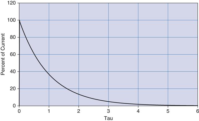
Notice how current can change immediately when the step input changes. Also notice how the voltage just doesn't change that fast. Capacitors impede a change in voltage, as the rule goes. What this also means is that changes in current⁸ will not be affected at all. Everything has its opposite, and capacitors are no exception, so let's move on to inductors.

Inductors Impede Changes in Current

Now that we have thought through the RC circuit, let's consider the RL circuit shown in Figure 2.10.

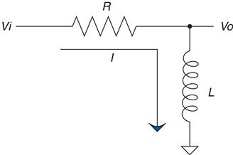
Remember that the inductor resists a change in current but not in voltage. Initially, with the same step input, the voltage at the output can jump right to 5 V. Current through the inductor is initially at 0, but now there is a voltage drop across it, so current has to start climbing. The current responds in the RL circuit exactly the same way voltage responds in the RC circuit.

Since you committed the RC response to memory, the RL response is easy. It is exactly the same from the viewpoint of current⁹⁹; the current graph looks like Figure 2.11 on the next page.

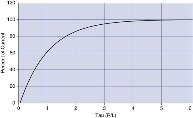
I hope you are saying to yourself, “What about the voltage response?” At this time, consider Ohm's Law for a moment and try to graph what the voltage will do. What is the current at time 0? How about a little later? Remember Ohm's Law—for the current to be low, resistance must be high. So initially the inductor acts like an open circuit. Voltage across the inductor will be at the same value as the input. As time goes on, the impedance of the inductor drops off, becoming a short, so voltage drops as well. Figure 2.12 shows the graph.

The inductor is the exact complement of the capacitor. What it does to current, the cap does to voltage, and vice versa.

Series and Parallel Components

There are two ways for components to be configured in a circuit:series and parallel. Series components line up one after another; parallel components are hooked up next to each other. Let's go over the formulas to simplify these component arrangements.

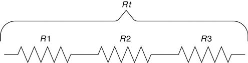
Series resistors, shown Figure 2.13, are easy; you simply add them up, no multiplication needed!

$\mathit{Rt}=R1+R2+R3$ Eq. 2.9

Eq. 2.9

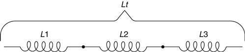
The inductors shown in Figure 2.14 are like resistors—you sum series inductors the same way.

$\mathit{Lt}=L1+L2+L3$ Eq. 2.10

Eq. 2.10

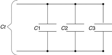
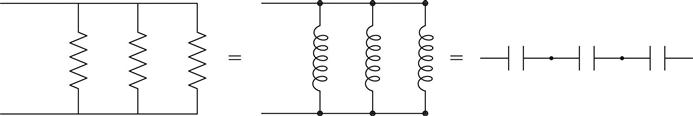
Remember that capacitors are the opposite of inductors. For this reason, capacitors must be in parallel to be summed up the way resistors and inductors are in series; see Figure 2.15 on the next page.

$\mathit{Ct}=C1+C2+C3$ Eq. 2.11

Eq. 2.11

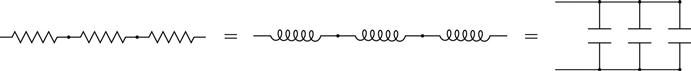
Remember the equivalences shown in Figure 2.16.

Parallel resistors, shown in Figure 2.17, are a little trickier. The equivalent resistance of any two components is determined by the product of the values divided by the sum of the values.¹⁰

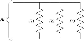
Keep in mind, however, that this works for any two resistors! In the case of three resistors or more, solve any two and repeat until done. (The // means in parallel with.)

$R1//R2=\frac{R1*R2}{R1+R2}\mathrm{ }\mathrm{ }\mathrm{ }\mathit{Rt}=\frac{R1//R2*R3}{R1//R2+R3}$ Eq. 2.12

Eq. 2.12

$L1//L2=\frac{L1*L2}{L1+L2}\mathrm{ }\mathrm{ }\mathrm{ }\mathit{Lt}=\frac{L1//L2*L3}{L1//L2+L3}$ Eq. 2.13

Eq. 2.13

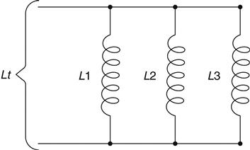
Parallel inductors are the same as resistors; you can reduce them in the same way—see Figure 2.18.

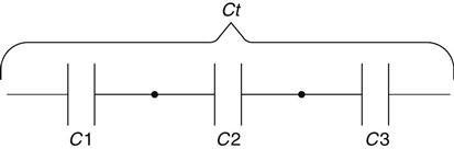
For capacitors the same equation applies, but only if they are in series, as shown in Figure 2.19. These are the circuits that use the product-over-the-sum, or the sum-of-the-inverses, rule¹¹; see Figure 2.20 on the next page.

$C1//C2=\frac{C1*C2}{C1+C2}\mathrm{ }\mathrm{ }\mathrm{ }\mathit{Ct}=\frac{C1//C2*C3}{C1//C2+C3}$ Eq. 2.14

Eq. 2.14

In dealing with parallel and series circuits, you can see that there are only two types of equations. One is simple addition, and the other is the product over the sum (or the sum of inverses). The only trick is to know which to use when. Remember that the resistor and inductor are part of the “in” crowd and the cap is the outcast wallflower who is the opposite of those other guys. I'll bet most engineers can relate to being the “capacitor” at a party, so this shouldn't be too hard to remember!

Thevenin's Theorem

Thevenizing is based on the idea of using superposition to analyze a circuit. When you have two different variables affecting an equation, making it difficult to analyze, you can use the technique of superposition to solve the equation, provided that you are dealing with linear equations (by luck all these basic components are linear; even if you might not think it when looking at the curve of an RC time response, it actually is a linear equation).¹²

The idea of superposition is simple: When you have multiple inputs affecting an output, you can analyze the effects of each input independently and add them together when you are all done to see what the output does. One idea that comes from superposition is Thevenin's Theorem.

Using Thevenin's Theorem allows you to reduce basically any circuit into a voltage divider. And we know how to solve a voltage divider, don't we! There is a sister theorem called Norton's, which does the same thing but is based on current rather than voltage. Since you can solve any electrical problem with either equation, I suggest you focus on one or the other. Since I like to think in terms of voltage, I prefer Thevenizing a circuit to the Norton equivalent. So to be true to the idea that you should only learn a few fundamentals and learn those well, we will focus on Thevenin equivalents.

The most important rule when Thevenizing is this:Voltage sources¹³are shorted, current sources are opened. Consider the circuit shown in Figure 2.21.¹⁴

Once all the voltage sources are shorted and all the current sources are opened, all the components will be in series or parallel. That makes it very convenient for those of us who only want to memorize a few equations! Apply those basic parallel and series rules we just learned and voilà, you have a circuit that is much easier to understand. Once you have reduced the resistors, inductors, and caps to a more controllable number, you replace each source one at a time to see the effects of each source on the component in question.

When you have considered the effects of each source one at a time, you can add them all together to see the overall effect. In this process of Thevenizing the circuit you are superimposing each output on top of the other to get the output of the combined inputs.

I find it helps when Thevenizing a circuit to try to imagine that you are looking back into the circuit from the output. This means that you imagine what the circuit looks like in terms of the output. We often think in terms of stuff that goes in the input. Something goes in, something happens, and then it comes out the output. Try flipping that notion on its head. Think, “Here is the output, what exactly is it hooked up to? What are the impedances that the cap in this case ‘sees’ connected to it?” Once you are able to adjust your point of view, Thevenizing will become an even more powerful tool. Consider the circuit shown in Figure 2.22.

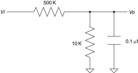
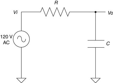
This circuit comes from a real live application. I would tell you what, but it is secret.¹⁵ So we won't say this is anything more than a voltage divider with a capacitive filter on it. (Values might have been changed to protect the innocent.)

This circuit's job is to lower a voltage at the input terminals varying from 0 to 100 V to something with a range of 0 to 5 V. The input voltage also has an AC component that is filtered out by the capacitor. The question is, what is the time constant of the RC filter in this circuit?

Is it 500 K*0.1 μf? That's what I would have thought before I understood Thevenin's Theorem. The output in this case is the voltage across the cap, so let's look back into the circuit to figure out what is hooked up to this cap. Now remember, I said there was a voltage source on the input of this circuit. Let's short that on our drawing and Thevenize it. Take a look at the Thevenized circuit shown in Figure 2.23.

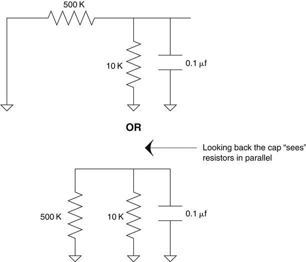
Hopefully at this point something really jumped out at you. The 10 K and the 500 K resistors are in parallel as far as the cap is concerned. Applying the rule of parallel resistors we find that the resistance hooked up to this cap is 9.8 K. Wow, that is a lot less than 500 K, isn't it! Thevenizing showed us that our first assumption was incorrect. In fact, the time constant¹⁶ of this circuit is much, much lower than it would be without the 10 K resistor.

There are other ways this theorem can be useful. Here is a case in point. You might have a circuit like the one shown in Figure 2.24 on the next page.

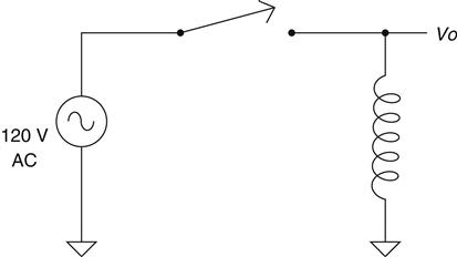
You need to switch AC power through this inductor (which was actually one winding of an AC motor in this case). Trouble is, when you let off the switch, a whole bunch of electrical noise is generated when this switch is opened. (We will discuss why when we cover magnetic fields later in the book.) A standard way to deal with this situation is with an RC circuit commonly known as a snubber. The point of a snubber is to snub this voltage spike and dissipate it as heat on the resistor. This makes the most sense if it is across the inductor, as shown in Figure 2.25.

Now let's apply Thevenin's Theorem to take a different look at this circuit, as shown in Figure 2.26. By shorting the AC voltage source, we quickly see that hooking the snubber up to the other side of the switch, to the AC hot line, would have exactly the same effect as hooking across the inductor. This fact once saved a company I worked for tens of thousands of dollars¹⁷ using the alternate location of the snubber circuit. I would say that makes Thevenizing a pretty powerful tool, wouldn't you?

It's about time

Constant Voltage Sources vs. Constant Current Sources

Devices that cause electrons to move are called sources since they are the source of electron or charge flow. The two typical types of source are ­voltage and current sources. Remember two important things when dealing with them.

The world of electronics is very voltage-centric, so you will see voltage sources much more often than current sources. This being the case, I will concentrate more on these types of sources.

Sources can come in two different types: AC or DC. Let's take a closer look.

Direct Current

The term direct current is used to describe current that flows in only one direction. I think this makes direct current the simplest to understand, so we should start there.

Direct current moves only one way, from positive to negative.²¹ A battery is a common direct-current device. Hooked up to a load such as a resistor, the current will go something like what's shown in Figure 2.27 on the next page.

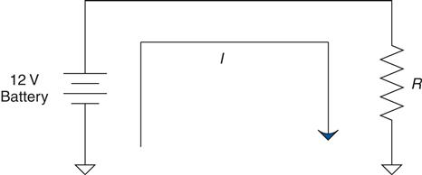
A battery²² is also a constant voltage device, so it will apply whatever current is needed to maintain its output voltage. So, we have 12 V hooked up to 1 Ω of resistance—hey, we just learned how to figure out current on a circuit like that! (More scribbling on a napkin…) That would be 12 amps of current.

A DC source will always try to move current in the same direction. One thing to note is that the current coming out of the source always needs to get back to the source somehow. The ground connection on the schematic should be thought of as a label that connects the signal back to the source. If the signal does not get back to the source, then there is no current flow.²³

Alternating Current

AC or alternating current came about as the interaction of magnets and electricity were discovered. In an AC circuit, the current repetitively changes direction every so often. That means current increases in flow to a peak, then decreases to zero current flow, then increases in flow in the opposite direction to a peak, then back to zero, and the whole process repeats. The current alternates the direction of flow in a sinusoidal fashion, so of course it is called alternating current. This type of current most commonly comes from big AC generators at your local hydroelectric dam.

AC power came into being due to this ease of generation—see Figure 2.28. When you move a coil of wire past a magnet, the current first climbs as the strength of the field increases, then as the field decreases and switches polarity, the current also decreases and switches polarity. The voltage and current change in a sinusoidal fashion naturally as the coil passes by the magnets.

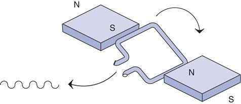
As long as you keep moving the coil, AC power will continue to be generated. You will see an AC source on a schematic represented by a sine wave squiggle like the one shown in Figure 2.29.

An interesting side note is that there was some argument when plans were being drawn up to distribute electricity across the United States. Edison (yeah, the famous light bulb guy) wanted to put small DC generators in everybody's home. Another lesser-known genius by the name of Tesla was pitching for AC distribution by wires from a central location. AC made some sense because the voltage could be easily transformed (yeah, you guessed it, with a transformer) from one level to another. That made it possible to jack up the voltage so high that the resistance of the distribution wires had little loss over long distances. There was much debate over the best setup.

One thing that tipped the scales in the direction we have today was the invention of the AC motor by Tesla. Till then only DC motors had been developed, and since this was before the diode, it wasn't so easy to make AC into DC. So being able to run a motor was a big deal. Although not as famous as Edison, Tesla²⁴ left a huge legacy in terms of AC power distributions and AC motors. Just look around your house and count up the AC motors in use. (Of course, there are a few light bulbs around, too.)

Back to Capacitors and Inductors Again

What was the rule of thumb for a capacitor? Capacitors impede a change in voltage. Do you remember the rule for inductors? Inductors impede a change in current. The flip side of these rules is that the cap will let current change all it wants and the inductor will let voltage change all it wants. One fact you can't ignore when it comes to AC sources is that current and voltage are always changing. How fast they change is a function of a term known as frequency. Frequency is the number of cycles of change per second; it has a unit called hertz. The higher the frequency, the faster the change in voltage and current. Now extrapolate for a moment what might happen to a cap in an AC circuit. It follows that a cap will block currents that have zero frequency (like a DC battery) and pass currents that change. The opposite applies to an inductor.

I like to think of it this way: The cap is an infinite resistor at DC or zero frequency. As frequency increases, the “resistance” (technically known as reactance) of the cap gets lower and lower, approaching zero. This capacitive reactance is known as X_C and is described by this equation. The unit is ohms, just like a resistor.

$X_c=\frac{1}{2\pi *f*C}$ Eq. 2.15

Eq. 2.15

The inductor is just the opposite. It starts with 0 Ω of resistance at a zero frequency and then increases to infinity along with the frequency. Inductive reactance is called X_L and follows this equation:

$X_L=2\pi *f*L$ Eq. 2.16

Eq. 2.16

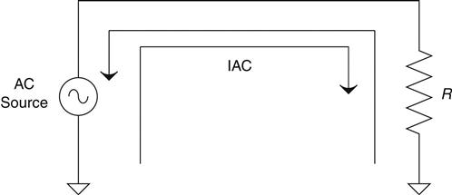
Let's hook them up to an AC source and vary the frequency to see how current flow is affected. This is easy enough to do in a spreadsheet. Simply plug the reactance equation into Ohm's Law. The schematic is shown in Figure 2.30.

Figure 2.31 shows what happens to current as frequency varies from zero (DC) to really fast (AC) when hooked up to a voltage source.

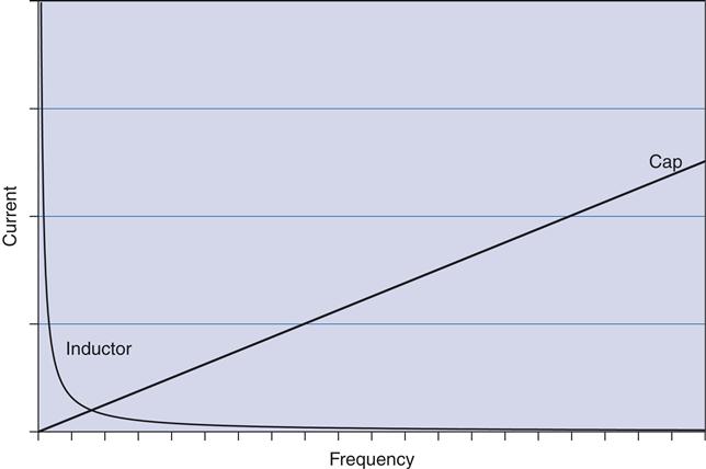
So to repeat, the higher the frequency, the easier the current wisll pass through a capacitor and the harder it becomes for it to get through an inductor.

You might be thinking, “What about that step input we put into the RC circuit before? How is it AC?” Actually, as weird as it might sound, it is AC. A really smart guy by the name of Fourier figured out some time ago that hidden in fast-changing signals are all sorts of high frequencies. He proved that the more abrupt the change in the signal, the more high frequencies that are present. An in-depth study of this topic is somewhat beyond the scope of this book, so let it suffice to say that the step input in the previous discussion has a sharp square corner, hidden in which are a whole bunch of high frequencies. These can't get through the cap, so the corner is knocked off, so to speak, leaving the characteristic curve that we saw as the transient response of the RC circuit.

Before we move on, we should touch on the topic of phase shifts. When both voltage and current are in sync, they are in phase. As we have discussed numerous times, inductors impede a change in current, but voltage is not affected, so if you graph the relationship between voltage and current, you will see that the change in current is a little out of sync with the change in voltage. It is said to be lagging behind. The capacitor has the opposite effect (as always), so the voltage is delayed relative to the current. In this case the change in current leads²⁵ the change in voltage. The current isn't magically jumping ahead of the voltage; the voltage is getting behind, but from the voltage point of view it looks like the current is changing first.

Capacitors and inductors are components that impede²⁶a signal, the amount of which depends on the frequency of the signal. The cap delays voltage changes, and the inductor delays current changes. They are opposite in the way they react to the frequency of a signal. Caps block lower frequencies while letting higher ones through, whereas inductors pass lower frequencies while blocking higher ones. Let's see what happens when we hook them up to a resistor.

Low-Pass Filters

Consider the circuit shown in Figure 2.32. Note similarities to the RC circuit that we used to first understand the effects of a capacitor. The difference is that now we are going to apply an AC signal to the input rather than the step input we applied before.

This circuit is known as a low-pass filter, and all you really need to know to understand it is the voltage-divider rule and how a capacitor reacts to frequency. If this were a simple voltage divider, you could figure out, based on the ratio of the resistors, how much voltage would appear at the output. Remember that the cap is like a resistor that depends on frequency and try to extrapolate what will happen as frequency sweeps from zero to infinity.

At low frequencies the cap doesn't pass much current, so the signal isn't affected much. As frequency increases, the cap will pass more and more current, shorting the output of the resistor to ground and dividing the output voltage to smaller and smaller levels. There is a magic point at which the output is half the input.²⁷It is when the frequency equals 1/RC. You might have noticed that this is the inverse of the time constant that we used earlier when we first looked at caps. Kinda cool when it all comes together, isn't it?

This is known as a low-pass filter because it passes low frequencies while reducing or attenuating high frequencies. You can make a low-pass filter with an inductor and resistor, too. Given that the inductor behaves in a way that is opposite of a capacitor, can you imagine what that might look like? Have a look at Figure 2.33.

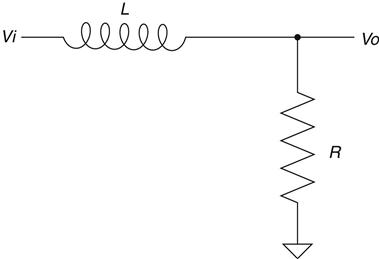
That's right; you swap the position of the components. That's because the inductor (being the opposite of a cap) passes the lower frequencies and blocks the higher frequencies. It performs the same function as the low-pass RC ­circuit but in a slightly different manner. You still have a voltage-divider circuit, but instead of the resistor-to-ground changing, the input resistor is changing. At low frequencies the inductor is a short, making the ground resistor of little effect. As frequencies increase, the inductor chokes²⁸ off the current, reacting in a way that makes the input element of the voltage divider seem like an increasingly large resistance. This in turn makes the resistor to ground have a much bigger say in the ratio of the voltage-divider circuit.

To summarize, in the low-pass filter circuits, as the frequencies sweep from low to high, the cap starts out as an open and moves to a short while the inductor starts out as a short and becomes an open. By positioning these components in opposite locations in the voltage-divider circuit, you create the same filtering effect. The ratio of the voltage divider in both types of filters decreases the output voltage as frequencies increase. All this lets the low frequencies pass and blocks the high frequencies. Now, what do you suspect might happen if we swap the position of the components in these circuits?

High-Pass Filters

Swapping the cap and the resistor in the low-pass circuit creates another type of circuit called a high-pass filter. Using your now supreme powers of deduction and intuition, you are thinking to yourself, “I'll bet that means the circuit passes high frequencies while blocking low ones.” You are correct, and the circuit looks like the one in Figure 2.34.

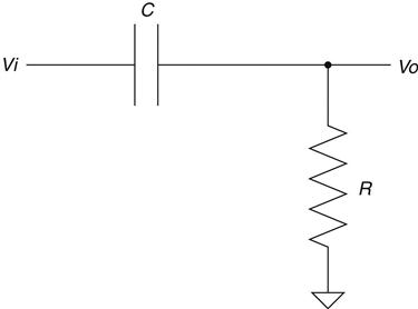
Hopefully, after our discussion on the low-pass circuit, the operation of this one is clear. The cap acts like a larger resistor at low frequencies, making the voltage divider knock down the output. At higher frequencies the cap passes more current as it becomes a short, causing a higher voltage at the output. The inductor version of this circuit looks like Figure 2.35.

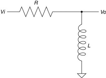
As you might have suspected, this filter is the inverse, circuit-wise, of the RC high-pass filter. Another little bit of serendipity is the fact that the half-voltage output point²⁹is also at 1/tau (tau means time constant generically, whether referring to an RC or an RL circuit), just like the low-pass filters.

To sum up, the high-pass and low-pass filters take advantage of the frequency response of either a capacitor or an inductor. This is done by combining them with a resistor to create a voltage divider that attenuates the unwanted frequencies while allowing the desired ones to pass. Some cool things happen when we put the two reactive elements together. You can create notch and band-pass filters where a specific band of frequencies is knocked out, or a specific band is passed while all others are blocked. The phenomenon of resonance also occurs in what is called a tank circuit, where you have a capacitor combined with an inductor. Just like the spring-mass example in Chapter 1 the tank circuit will oscillate current back and forth from one component to the other.

Active Filters

So far we have been studying passive filters. A passive component is one that is not powered externally. Being passive, these components are subject to an effect known as loading. This means that anything you hook up to the output can affect the performance of the filter. Take a low-pass RC filter, for example, and hook a resistor up to it, as shown in Figure 2.36.

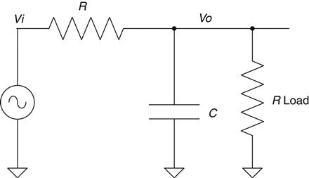
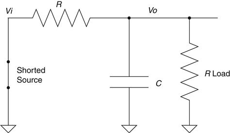
This resistor on the output is a load. It could be another part of the circuit or any number of things, but the point is that it acts like a resistor to ground. How does this affect the RC filter performance? To understand, let's Thevenize it to “see” how the load affects the output. We start by shorting the voltage source to ground. This is done with AC sources the same as DC, so the circuit would look like Figure 2.37.

Because I like my examples to use real numbers,³⁰ let's make up some values. Let R=10 K and let Rload=10 K and C=0.1 μf.

When you Thevenize a circuit, you reduce all the parts into one, where possible. In this case the resistors are in parallel, so apply the parallel rule to the resistors and you get a value of 5 KΩ. Did you notice that the R value has changed considerably due to the load on the circuit? What might seem counterintuitive at first is the fact that the time constant of this circuit is a function of the Thevenized version that we just derived. So, without the load, tau would have been 10 K×0.1 μs, or 1 ms.

With the load, it is 0.5 ms, half what it was before! Since the output of this filter depends on τ, we can see that the load has affected it significantly. A way to avoid this problem is to add an active component to the design, making it into an “active” filter. In adding such a component, the basic idea is to minimize this loading effect to a point that you get a nice predictable response. The output of the active filter is such that no matter what load you put on it, it does not affect the response of the filter—see Figure 2.38.

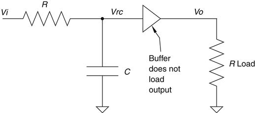
The input of this active device (known as an op-amp) has a very high impedance. In this case it is comparable to a 10-meg resistor. Hooking that up to the RC filter will have little effect on the time constant of this circuit as long is it is significantly larger³¹ than the R value in the circuit. The buffer in this circuit will output a voltage that matches the voltage on the input. It will buffer the signal; no matter what you hook up to the output, the filter will not be affected. This is one of the simplest active filters, but the principle with all of them is the same—include an active element to preserve or enhance the integrity of the filter.

Beam Me Up?

Electrons are everywhere, or maybe it is better said that the effects of electrons are everywhere. There are invisible fields of force all around us that are caused by those pesky little devils. These fields warrant discussion because they are a factor in the way we deal with electricity. They can store energy and affect the world around them in various ways, so it is good to build an intimate knowledge of these fields and how they interact. These are the same fields that we talked about in the newly added Chapter 0 of this edition. If you elected to skip it when you started reading and you feel a little lost here, I suggest going back to read that chapter.

Now, we can't beam people³² on and off the planet like they do on Star Trek, but there are couple of invisible fields that are what actually create all the effects that we see in electric circuits. It is these fields that make the water, ping-pong ball, and many other analogies not quite match what is really going on in a circuit. So understanding these fields will definitely help develop the intuitive skills we are working on.

The Magnetic Field

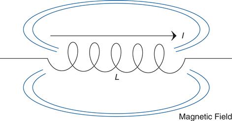
This is the most well-known of the two fields that we are going to discuss. Who hasn't experienced the force of a magnet sticking a note to the fridge or felt the power of two repelling magnets? Back in the 1820s, a man by the name of Hans Oersted noticed his compass read strangely every time he switched on a current in a wire. Eventually it was figured out that a moving electron (such as the current in a wire) creates a magnetic field perpendicular to the direction of electron movement, as shown in Figure 2.39.

This field is identical to the field surrounding a permanent magnet. In fact, if you coil the wire like what's shown in Figure 2.40, the magnetic field lines align and reinforce each other, making it even more like a permanent magnet.³³

Electromagnets, as they are called, are pretty cool since they can be switched on and off, unlike permanent magnets. Another important fact is that not only does a current moving through a wire create a magnetic field, but the opposite is also true. A changing magnetic field can create or induce a current in a wire. A coil of wire is known as an inductor for this reason. Energy is stored in an inductor as a magnetic field. It is like a rubber band that is stretched as you apply current. When the current is shut off it snaps back, and energy is given up as the magnetic field collapses (it is changing as it goes away). This collapse induces a current in the wire. Consider the circuit shown in Figure 2.41.

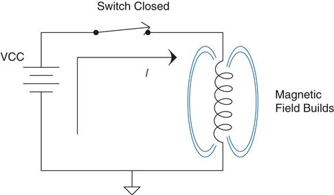
When the switch is closed, current flows and a magnetic field is created. It is the creation of the magnetic field (stretching the rubber band, so to speak) that causes the inductor to “resist”³⁴the change in current, as we learned it does earlier. The flip side of that also happens. If we open the switch, the change in the field as it collapses would like to keep the current flowing in the inductor—see Figure 2.42.

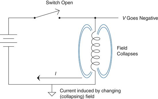
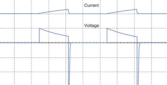
If there is no place for this current to go, the voltage across the inductor will increase instantaneously and then dissipate as the induced current drops off with the drop of the magnetic field. Take a look at the graph shown in Figure 2.43 of the current and voltage changing in this inductor circuit as the switch opens and closes.

Induction is also the fundamental principle that a transformer uses. The magnetic field—as it is created on one side of the transformer as is shown in Figure 2.44—induces a current on the other side of the transformer. When the field reduces, and it switches direction, a corresponding current is induced at the output.

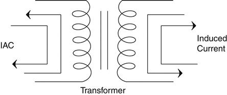
The ratio of turns on each side of the transformer controls the ratio of voltage from input to output. A 101 ratio will take 120 V on one side and create 12 V on the other. Note also that though voltage goes down, current goes up, making a transformer kind of like a gear train or lever in the mechanical world. Power into it is the same as power out of it (minus losses, of course). Voltage times current in equals voltage times current out. This is akin to the rule of force times distance on one side of a lever equals force times distance on the other side.

The fundamental component of a transformer is an inductor. An inductor is simply a coil of wire, as we learned earlier. The number of turns of wire controls the concentration of the magnetic field. The core of the inductor also has the effect of concentrating the field. The material in the core can become saturated,³⁵ meaning that it cannot concentrate the field any more tightly than it has.

The important things to remember are that current creates a magnetic field, and a changing magnetic field creates a current. The changing field can be externally applied from a moving magnet, the input side of a transformer, or from the collapse of the field just created by the current. Current and magnetic fields are closely connected.

The Electric Field

Also called the electrostatic field, the electric field³⁶ is not as commonly known perse as the magnetic field. In the same way that current is connected to the magnetic field, voltage is connected to the electric field. That leads to a good rule of thumb to remember:Current is magnetic and voltage is electric.

The electric field comes from electric charges, both positive and negative. In a way that is analogous to the way like poles on magnets repel and opposite poles attract, like charges repel and opposite charges attract. Any molecule or atom can be neutral (no net charge), positively charged, or negatively charged. The accumulation of these charges is what is known as voltage. One way to think of it is that the charges are the voltage making the electric field, and movement of those charges is called current and creates the magnetic field.

Similarly to the way an inductor is a way of concentrating a magnetic field, a capacitor is a way of concentrating an electric field. Capacitors are made by two collectors or plates separated by a material that will not conduct electricity, also known as a dielectric. The symbol of a capacitor mimics the construction, shown in Figure 2.45.

Because of the dielectric, current or actual charges cannot flow or move across the capacitor, all the charges build up on one side of the cap, kind of like a 50-car pileup on the freeway, as shown in Figure 2.46.

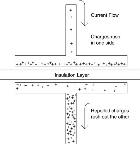
As the charges pile up on one side, the electrostatic field builds up, causing all the like charges on the other side of the cap to go rushing away (remember how like charges repel). Once it all comes to rest, there is an equal number of opposite charges on the other side of the cap. In this way the capacitor stores a charge of voltage on the plates of the capacitor.

How much charge a cap can store in an electric field is a function of the area of the plates. The amount of voltage it can store is dependent on the strength of the dielectric. If you exceed the capability of the insulation, the dielectric will break down and a charge will cross the gap. The same thing happens on a stormy day. During a thunderstorm charges build up in the clouds and the ground in the same way they do on either side of a capacitor. A lightning strike is a large-scale version of what happens when the insulation or dielectric in a capacitor breaks down.

In the same way current creates a magnetic field, voltage creates an electric field. Just as the magnetic field can store energy, the electric field can also store energy. As the magnetic field dissipates, it tries to maintain current. As the electric field dissipates, it tries to maintain voltage. Voltage and electric fields are closely connected.

Thumb Rules

• An inductor stores energy in a magnetic field.

• A capacitor stores energy in an electric field.

• Current is magnetic.

• Voltage is electric.

Keep It Under Control

The topic of control theory is typically left till later in most education programs because it is considered a more advanced topic. Control systems, however, are a very common application in the electronic realm. Think about it; i'll bet most of the time you design a device to control something you don't want to think about, something that automatically does what it should without intervention. On top of that, control theory turns out to be useful in more than just clear-cut control applications—understanding op-amps and designing power supplies, for example. Since a basic knowledge of this concept will help you in many aspects of your career, it seems prudent to dedicate a few pages to it.

The System Concept

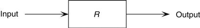
A system is anything with an input and an output. The idea is simple—take the input, shake it, squeeze it, do whatever, and then send it to the output. It can be represented with a block diagram, something like the one shown in Figure 2.47.

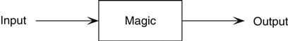
All the magic happens inside the box. This magic is called the transfer function. The transfer function is equal to the input over the output. It is the equation that you process the input through to get the output, so the following is true:

$\mathit{Output}=\mathit{Magic}*\mathit{Input}$ Eq. 2.17

Eq. 2.17

A little algebra yields:

$\frac{\mathit{Output}}{\mathit{Input}}=\mathit{Magic}$ Eq. 2.18

Eq. 2.18

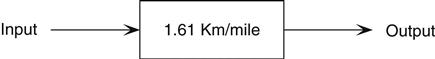
Now you know how to find what the magic inside the box is, and sometimes it is just that easy. Let's try a simple example to see how. You put 12 miles into the input, wait…chugga, chugga, ding!…and out pops 19.32 km. As you might have guessed, the magic in this box is a metric converter, but what is the transfer function? According to the preceding equation, we simply divide the output by the input. That would be:

$\frac{19.32\mathit{km}}{12\mathit{miles}}=1.61\frac{\mathit{km}}{\mathit{mile}}$ Eq. 2.19

Eq. 2.19

The magic in our converter box looks like the one in Figure 2.48.

Note that the units made it into the box. This helps identify the type of units that will work at the input and what you will get at the output. Hopefully a little voice in your head is saying, “Isn't this a rehash of the unit math chapter?” It is, but this is a more formalized concept with some neat touches such as the cool little boxes³⁷ you draw to help you understand the system. The next question you should ask is, “How does this apply to electronics?” Well, from the most basic to the most complex, you can represent any circuit with one of these magic (okay, some texts call them black) boxes

we'd better do another example. Take a resistor. A resistor can be thought of as a current-to-voltage converter. Put current into the input, apply magic, and get voltage at the output. What would be the transfer function of that? If you mumbled a phrase with the words Ohm's Law anywhere in it, you are probably right.

$R=\frac{V}{I}$ Eq. 2.20

Eq. 2.20

That would make the block diagram of the resistor look something what Figure 2.49 shows.

In this transfer function, R is the value of the resistor in ohms, just in case you didn't guess. (Note that 1 unit of ohms equals 1 unit of volts divided by 1 unit of amps, like good old Ohm's Law says it does.)

Let's step up the idea to something a little more complex, like a voltage divider. We already know the equation for this. It is:

$\mathit{Vo}=\mathit{Vi}\frac{\mathit{Rg}}{\mathit{Rg}+\mathit{Ri}}$ Eq. 2.21

Eq. 2.21

Do you remember what Vo stands for? How about Vi? They are voltage output and voltage input. So let's just use a little algebra to figure this out. The transfer function is equal to the output over the input, like this:

$\frac{\mathit{Vo}}{\mathit{Vi}}=\frac{\mathit{Rg}}{\mathit{Rg}+\mathit{Ri}}$ Eq. 2.22

Eq. 2.22

The block diagram would look like Figure 2.50.

This same concept can be used to describe all the circuits that we have seen so far. You might see block diagrams of this type where C or L has a little s by it. This is a mathematical trick known as a Laplace transform. It is used to simplify problem solving. If you transform all that time constant and frequency stuff using Laplace pairs, you can treat the transformed equations with simple algebra and then transform it all back when you are done. Laplace transforms are beyond the scope of this text, but do take note that the s rolls up all the frequency response of capacitors and inductors into a domain that can be handled easily when the equations get complex.

We can describe any system as a magic box with an input and an output. One way to determine what is in the magic box is to put a known signal into the input. take a look at what is probably the most important stimulus you can apply to the input of the magic box.

The Step Input

The idea behind the step input is to understand the output of a system by its response to a given input. The step input is an instantaneous change of state from a value of zero to another predetermined value. It looks like the one shown in Figure 2.51.

The output will change in some manner predictable (one hopes!) by an equation. This is known as the response. The better you know the response of various components to this step input, the better you will be able to apply intuitive signal analysis. Let's go over the RC circuit again. The equation we learned earlier is:

$\mathit{Vo}=\mathit{Vi}\left(1-e^{-\frac{\tau }{\mathit{rc}}}\right)$ Eq. 2.23

Eq. 2.23

To turn that into the transfer function for the magic box, all we have to do is move Vi to the other side of the equal sign, like this:

$\frac{\mathit{Vo}}{\mathit{Vi}}=\left(1-e^{-\frac{\tau }{\mathit{rc}}}\right)$ Eq. 2.24

Eq. 2.24

We now plug that into the box. When we put the step input into one side, we get the familiar RC curve on the output, as shown in Figure 2.52.

Though it is nice to see the same conclusion from a different approach, where the system concept comes into its own is when we create a feedback loop.