New methods and instruments for performance and durability assessment
M. Röger*; C. Prahl*; J. Pernpeintner†; F. Sutter† * German Aerospace Center (DLR), Almería, Spain
† German Aerospace Center (DLR), Cologne, Germany
Abstract
This chapter describes new methods and instruments for performance and durability assessment of concentrating solar power (CSP) systems. It comprises point and line focusing systems, and presents new methods on both the component level (heliostats, thermal receivers, and rotation and expansion performing assemblies) and the system level.
Keywords
Concentrating solar power; CSP; Solar receiver; Solar concentrator; Qualification methods; Durability assessment; Measurement; Component performance; System performance
7.1 Component performance
7.1.1 Outdoor testing of receiver solar absorptance
Two basic approaches exist to derive receiver solar absorptance. The first approach is to measure an enthalpy difference of a medium inside the receiver and the receiver itself by irradiating it with lamps or the sun (see Table 7.1). The second approach is to measure directly the reflectance of glass envelope and absorptance of the selective coating (Table 7.2). While the first approach usually includes the whole receiver assembly, which is important for product qualification, the second approach is a more direct measurement of the properties α and τ of the receiver which have a major influence on receiver performance. Fig. 7.1 shows three outdoor test benches.

Table 7.1
Indirect, nondestructive measurement of solar absorptance of a solar receiver assembly by measuring a change in enthalpy
| OptiRec/ElliRec DLR [1,2] | SolaRec DLR/KONTAS [2,3] | Parabolic Trough, e.g. [4] | Dynamic techn. NREL [5] | |
| Indoor/outdoor | Indoor | Outdoor | Outdoor | Outdoor |
| Light source | Metal halide lamps | Sun | Sun | Sun |
| Stationary/dynamic | Stationary | Stationary | Stationary | Dynamic |
| Concentration | Concentrating | Concentrating | Concentrating | Nonconcentrating |
| Tracking | Nontracking | 2D-tracking | 1D-tracking | Nontracking |

Table 7.2
Direct, nondestructive measurement of spectral properties of selective coating absorptance and glass envelope transmittance (α, τ) of a solar receiver by measuring reflectance and absorptance
| Mini Incus Abengoa [6] | Test bench CENER [7] | Integration cylinder Fraunhofer ISE [8] | |
| Indoor/outdoor | Outdoor, solar field | Indoor | Indoor |
| Light source | LEDs | White light and wavelength scanning | White light in integrating cylinder |
| Detector | Photodiodes | Spectrophotometer | Spectrophotometer |
| Wavelengths | 365-1950 nm | 300–2500 nm | No information |

The indoor OptiRec [1] and ElliRec [2] test benches, the outdoor two-axis tracking SolaRec [2] or KONTAS [3] test benches or a typical one-axis tracking parabolic trough [4] can be used to measure the temperature increase of the fluid flow inside the receivers. The heat transferred to the heat transfer fluid in the receiver ![]() is the optical receiver efficiency ηopt,rec times the concentrated solar light incident on the receiver
is the optical receiver efficiency ηopt,rec times the concentrated solar light incident on the receiver ![]() , reduced by the thermal loss
, reduced by the thermal loss ![]() :
:
If the receiver is operated at near ambient temperature, the heat loss is zero. Hence, the optical receiver efficiency can be measured by estimating the intercepted solar radiation on the receiver and measuring the enthalpy increase in the fluid flow inside the receiver. For perpendicular incidence of solar radiation:
For perpendicular incidence of solar radiation, the receiver efficiency is
while Pd accounts for the power due to absorbed diffuse radiation, ρ for the mirror reflectance, χ for the cleanliness, and γ for the intercept factor. If measured outdoors and with small aperture concentrators, this term is not negligible. The optical receiver efficiency is an integral over the whole receiver assembly, including the bellow regions.
The DLR ElliRec (1st generation test bench [2]) and OptiRec (2nd generation test bench [1]) use metal halide lamps and concentrators in a laboratory environment to heat water. A homogeneous absorber temperature is reached by inserting a displacement cylinder with a helical wire on its surface inside the receiver. The indoor test bench has the advantage that no tracking and no sun are necessary; there are no transients by clouds or variable energy input due to tracking errors or soiling. However, the lamps' spectral composition differs from that of solar radiation.
The DLR SolaRec [2] and the KONTAS [3] at the PSA are two-axis tracking parabolic troughs using solar radiation. The SolaRec consists of two parabolic troughs mounted on a two-axis tracking Helioman tracker. Each trough has an aperture of 2.3 m and a length of 5 m. The mass flow rate, the small temperature difference over the receiver, heat losses in the piping, the tracking influencing the intercept factor, mirror reflectance and cleanliness, and the accurate consideration of direct normal irradiance (DNI) and the absorbed diffuse radiation have to be accounted for. An absolute 2σ measurement uncertainty of 3.6% is reported for the optical receiver efficiency, a relative comparison with a reference receiver mounted on the same SolaRec test bench yields to an absolute 2σ measurement uncertainty of 1.3% [9].
The same procedure can be applied to receivers mounted on the rotary test bench KONTAS at the Plataforma Solar de Almería. Here, a EuroTrough-type collector module (aperture, 5.76 m, length 12 m) is mounted on an azimuthal tracker. Three receivers are mounted in the focal line and Syltherm as heat transfer fluid is used. As having a larger concentration ratio and three receivers mounted, the temperature increase is higher and hence measurable with higher accuracy. A mixer is mounted upstream of three calibrated PT-100 temperature sensors both at inlet and outlet. However, the specific heat capacity of the organic heat transfer fluid is not as stable as pure water and hence only known with uncertainties not better than 5%. For that reason, an online calorimetric cp-measurement [10] is included with an uncertainty of about 1%. The mass flow rate device is a highly accurate Coriolis sensor. The intercept factor is determined by a deflectometric slope deviation measurement and subsequent raytracing. The determination of the intercept factor is necessary because operating near ambient temperature the receiver tubes do not totally lie in the focal line of the concentrator as they do at operating temperature in a parabolic trough plant. The second reason is that the concentration ratio is higher than in the SolaRec test bench and not all rays may hit the tube.
One-axis tracking east-west mounted parabolic trough loops can also be used to approximately derive receiver optical properties as reported in Ref. [4].
While concentrating setups have to cope for accurate tracking and accurate determination of intercept factor, reflectance, and cleanliness, the nonconcentrating setup proposed by NREL [5] does not have these disadvantages, although the flux profile on the receiver differs from its later application in concentrating collectors. Instead of cooling the receiver by an internal mass flow and measure steady-state, NREL proposes a dynamic technique and observes the temperature increase after perpendicular exposure of the receiver to nonconcentrated sunlight. By observing the slopes of temperatures over time of the steel absorber tube and the materials filled inside (i), the product τα can be calculated.
while ![]() is the power of direct and diffuse radiation to which the receiver is exposed. This technique also avoids highly precise absolute temperature measurements. The optical receiver efficiency can be approximated by the following equation:
is the power of direct and diffuse radiation to which the receiver is exposed. This technique also avoids highly precise absolute temperature measurements. The optical receiver efficiency can be approximated by the following equation:

To ensure a slower heat-up of the receiver after exposure to sunlight, to avoid receiver damage and homogenize temperatures, an aluminum tube is inserted into the receiver and the remaining annulus between absorber and aluminum tube is filled with fine aluminum shot. Various thermocouples record the temperature rise in the different sections. The thermal capacitance values for the aluminum shot, the aluminum tube, the absorber steel tube, and the thermocouple wiring and sheathing are taken into account.
The highest uncertainty is the accurate determination of the solar radiation incident on the receiver, because apart from the direct radiation, a significant part of diffuse radiation comes from the sky and the surroundings. To increase the amount of direct radiation during the test, a white shroud with 5.08 cm opening is used to prevent diffuse radiation to reach the receiver. A pyranometer aligned with the receiver was located under an aperture similar to the shroud used to measure the incident radiation on the receiver. Here are the major uncertainties of the method, because still diffuse radiation reaches the receiver and it is difficult to expose the pyranometer to the same radiation as the receiver due to the glass envelope of the receiver. NREL reports a measurement accuracy of ±3.4%. As in the other test benches, a higher accuracy is reached, if a comparative, parallel measurement is done relative to a reference receiver.
The second approach to determine the solar receiver absorptance is the direct measurement of the properties α and τ of the receiver (Table 7.2).
The portable, battery-powered “Mini Incus” spectrophotometer of the company Abengoa Solar for use in a solar field uses LEDs and photodiodes to measure in 14 different wavelengths over the solar spectrum [365–1950 nm] in two main optical paths [6]. One optical path measures the transmittance of the receiver glass envelope tube. The other path measures the reflectance of the absorber tube, thus the spectral absorptivity can be derived. Abengoa Solar states a 3σ uncertainty of ±1.0% for τ and ±0.3% for α. Successful measurements glass envelope transmittance in a solar field are reported, e.g., in Ref. [11].
CENER designed a laboratory test bench in which the receivers can be heated and rotated optionally [7]. The underlying concept is similar to that of the “Mini Incus.” It uses a unique light source and wavelength scanning module to produce two light beams for glass envelope transmittance measurement and absorber tube reflectance. After transmittance/reflectance on the receivers, the light beams are conducted by optical fibers to the optical sensor heads (Si and InGaAs) to cover the spectral range from 300 to 2500 nm.
The “Mini Incus” and the CENER test bench assume a nondiffuse reflection of light on both the glass envelope and the selective coating. This assumption has to be checked before applying the techniques. Different concepts which do not rely on a specular reflection have been investigated theoretically in the PARESO project [12]. One concept uses integrated spheres and cylinders. Fraunhofer ISE built a measurement bench using an integration cylinder and a white light source [8]. By shifting a partly reflecting and partly absorbing plate inside the cylinder, spectra can be recorded, in which the reflection of the glass envelope tube can be separated from the reflection of the absorber tube.
7.1.2 Measurement of receiver heat loss in the solar field
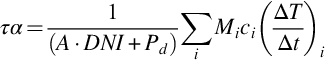
Receiver heat loss in the solar field plays an important role in the energetic and economic performance of a parabolic trough solar power plant. The heat loss of an evacuated parabolic trough receiver ranges typically between 150 and 200 W/m for receivers with 70 mm absorber tube diameter at 350°C [13–15]. Yearly heat loss of about 7% (Ma’an, Jordan) to 10% (Guadix, Spain) of the collected solar energy is calculated for a EuroTrough-type collector [16]. Receivers are designed to serve the whole plant operating time, at least 20–40 years, without suffering significant performance loss. However, different technological maturity of receiver products, lack of experience in operation and maintenance of parabolic trough plants and their heat transfer fluids, and increasing temperature using new fluids as salts put receiver performance at risk over the plant operating time. Defects such as vacuum loss, glass breakage, and coating degradation may decrease the annual electricity production because thermal losses increase by a factor of 5–10. A sudden accumulation of hydrogen in the receiver annulus can be caused by constant diffusion of hydrogen from the heat transfer fluid through the absorber tube and getter saturation [17–20]. A saturation of the getter can occur due to excessive hydrogen concentration in the heat transfer fluid or in the case of substandard receivers with reduced getter capacity. Fig. 7.2 shows the typical specific heat loss of intact and defective receivers.
Field measurement techniques to qualify mounted receivers are associated with additional constraints in comparison to laboratory measurement techniques. They have to be nondestructive, prohibiting a direct access to the solar selective coating, getter components, and evacuated annulus. Moreover, these field techniques must be robust and reliable at a reasonable accuracy which can be challenging under variable environmental conditions. Screening methods must be fast due to the large amount of receivers in parabolic trough field. The Spanish 50 MW Andasol-3 plant has 22,464 installed receivers, for example.
Visual inspection techniques are the least accurate, but they allow an early detection of receiver defects. If properly activated, the flashed evaporable getters act as a qualitative vacuum indicator, turning white in the case of air leakage, but they do not react with hydrogen. In addition, the selective coating can be checked for inhomogeneity, scratches, peeling, or oxidation. The glass envelope can be checked for breakage.
The glass temperature can serve as an indicator of the receiver quality. Passive IR thermography techniques [21–23] record the glass envelope temperature as a function of absorber temperature, which is either measured with a solar blind IR sensor [24] or assumed to increase linearly as a function of HCE position in the loop. The glass temperature as indicator of the receiver quality can be measured with a broad range of IR sensors, such as miniaturized pyrometers or uncooled bolometers, being sensitive in the wavelength range between 8 and 14 μm. Alternatively, solar blind IR cameras which are not affected by incident solar radiation and being sensitive in the wavelength range between 0.3 and 2 μm can be used [25].
Price et al. [21] present data of a solar field survey using temperature measurements of the glass envelope based on infrared thermography to qualify the thermal quality of the receivers. Receivers with hydrogen accumulation could be easily distinguished from intact receivers.
The handheld “Thermohook” is a device from the company Abengoa Solar which is manually hooked over the receiver by a worker. Absorber tube and glass envelope temperatures are measured together with ambient temperatures. The “Thermal Scout” of NREL [23] is a truck mounted solution to measure the glass envelope temperatures and associate them to GPS data. Even faster is an airborne system, e.g., the QFly-Thermo system of DLR which uses an infrared camera mounted on a quadrocopter. The system generates GPS-referenced glass temperature maps of the receivers.
The infrared measurements should only be done at low wind conditions, because the same glass envelope temperature may be measured for two receivers having different heat losses. For example, assuming an ambient temperature of 25°C and an absorber temperature of 350°C, numerical simulations show that a standard receiver without forced convection has a specific heat loss of 150 W/m and a glass temperature of 58°C. Roughly the same glass envelope temperature is measured for a defect receiver (air intrusion into vacuum) with a specific heat loss of approximately 514 W/m at an air speed of 6 m/s near the glass envelope. For this reason, the technique to survey solar fields by infrared thermography is a good screening technique, but does not deliver accurate quantitative heat loss results.
Once a fast screening of the glass temperatures is done, some receivers might be inspected for more quantitative results. Active IR thermography is a field measurement technique with a high level of complexity, but also a high depth of information. The receiver specific heat loss is determined by applying a thermal excitation to the absorber tube and by measuring both the absorber and glass temperature response signals with infrared pyrometers. These temperature signals and the ambient temperature are used to identify receiver thermal properties like heat loss, vacuum quality, and selective coating emittance. They are evaluated with the help of a numerical heat transfer model coupled to a parameter identification algorithm. This method provides insight into the receiver degradation mechanisms [26].
The measurement system consists of two IR sensors to measure dynamic variations of absorber and glass envelope temperature, a ventilated cylindrical radiation shield, and some thermocouple sensors for temperature monitoring [27,28], see Fig. 7.3. The pyrometer for absorber temperature measurement has a sensor range from 2.0 to 2.6 μm, the pyrometer for glass temperature measurement from 8 to 14 μm. The 1 m long equipment is mounted like a shell around the receiver of a defocused collector and the absorber temperature is excited. In a solar field, the temperature excitation can be achieved either by adjusting the mass flow or by focusing or defocusing upstream collector units for tests during the day. Fig. 7.4 exemplarily shows simulated temperature variations of the absorber tube and glass envelope of intact receivers at different positions in a loop after defocusing of the first collector. The excitation is sufficient to derive the receiver properties.


As this is an indirect method, the results of the transient measurements are input for an inverse heat transfer problem [28] using the dynamic model equations described in Ref. [26] to identify the thermal parameters coating emittance and annulus heat transfer. These can be used to calculate receiver heat losses at any conditions required.
Transient measurements with different receiver samples with state-of-the-art coatings and vacuum, but also samples without vacuum and absorber tubes painted with normal black paint, are compared to ThermoRec indoor reference measurements (see Chapter 4). The laboratory proof of principle and validation are described in Ref. [27]. The observed specific heat loss deviations between steady-state and transient laboratory measurements range from 2% to 4% for evacuated receivers with selective coating and from 1% to 9% for receivers with black painted absorbers, respectively. The technique also is validated under field conditions at the KONTAS facility; see Fig. 7.5 [28]. Under field conditions, the method allows a correct estimation of specific heat losses within an accuracy range below ±10% for all tested receivers. Relevant separation of heat loss mechanisms could be derived for standard receivers, while only partially biased diagnoses could be observed for partially or non-evacuated PTRs with highly emissive absorber coatings.

A further technique using microwave induced plasma and analytical spectroscopy [29] seeks to extract information about possible gases in the annulus between absorber and glass tube. This technique allows both a qualitative and quantitative analysis inside a certain pressure range in which the annulus gases form a plasma. The gas type can be identified by the emission spectra of the plasma. However, if the plasma does not ignite, the result is not unambiguous. In this case, the receiver annulus space could be either intact or filled with a gas having a pressure too high for plasma ignition.
7.1.3 Measurement of performance of receiver selective coatings
The thermal emittance ɛabs of the selective coating of a parabolic trough receiver has major importance regarding the performance, especially at high temperatures. Its value can be measured using calorimetric methods or spectrometric methods. The latter (see e.g., [30]) are limited to selective coatings samples without glass envelope, because the glass envelope of the receiver does not transmit radiation with wavelengths higher than approximately 2.7 μm, and the emittance of the selective coating must be known up to 25 μm. If the samples are heated, the coatings may have to be protected from oxidation.
The steady-state calorimetric measurement of emittance has the advantage that it avoids all issues typically associated with spectrophotometric reflectance measurements. Furthermore, the sample is at the target temperature during the measurement so that the change of emittance with temperature is automatically included into the results. For this reason, various test methods and special test benches are developed to measure the coating emittance by calorimetric methods.
Two basic approaches regarding calorimetric measurements can be distinguished. The first approach heats a coated absorber tube or a coated sample without glass envelope in a vacuum chamber and the heating power and temperatures of the absorber sample and surroundings are measured. The second approach heats a whole receiver assembly (including glazing) and measures the heating power and temperatures of the absorber and glass envelope tube. The second approach preferably is done in a vacuum chamber [31], but corrections available in near future may be applied to achieve good measurement accuracy also without vacuum chamber.
7.1.3.1 Coated absorber tube or a coated sample without glass envelope
The following section describes a setup being developed at DLR to characterize absorber tubes without glass glazing or flat coating samples. The total hemispherical emittance ɛabs is measured by heating the sample with electrical heaters inside a vacuum chamber to a target temperature and measuring the heat loss and temperatures of both the sample and its surroundings. Convection losses can be neglected and heating power is equal to the sum of radiation loss and conduction via the sample supports. The method can be used with flat samples, but is also suitable for tubular samples, which are the primary focus of this section [32–34].
The electrical heaters are placed inside tubular samples with the relevant coating at the outer surface. Fig. 7.6 shows the cylindrical sample (1) surrounded by an artificial sky (2). Both surfaces are characterized by emittance ɛ, temperature T, and area A.

Approximating the configuration as concentric cylinders of infinite length, gray bodies (![]() ), and diffuse reflection at surface 2 and specular reflection at surface 1, the net-heat flux P1−2 from sample (1) to artificial sky (2) can be calculated by [35].
), and diffuse reflection at surface 2 and specular reflection at surface 1, the net-heat flux P1−2 from sample (1) to artificial sky (2) can be calculated by [35].

As the gray body approximation is inadequate for selective surfaces, the radiative fluxes from surface 1 to surface 2 and from surface 2 to surface 1 are considered separately in Eq. (7.7). Hence the equation contains emittances at both radiator temperatures T1 and T2:

Solving for the emittance of the sample at the temperature of the sample leads to the following equation:

The inside surface of the artificial sky, coated with a high emittance coating, is cooled with water or liquid nitrogen to a low temperature. The axial end faces of the tubular sample are covered with insulation or counter heaters or both in order to keep axial radiative heat loss low. Counter heaters covering the cables for thermocouples and heaters can be used to suppress heat conduction loss via the cables of heater and thermocouples.
The temperature of the coating can be measured with thermocouples that are pressed on the inner absorber tube surface. As they are placed in the annulus between absorber and heater, the thermocouples are influenced by thermal conduction via the cables and the radiation temperature. Hence these measurements show a temperature that is higher than the temperature of the absorber outer surface. This systematic effect must be considered and a corrective temperature difference ΔT has to be applied.
For this, a reference absorber tube is used. It is equipped with additional thermocouples which are soldered or welded on the outer absorber surface at the points where the inner thermocouples are located. The temperature difference between inner and outer thermocouples ΔT is measured using the original sample heater as a function of temperature T and heat loss. In order to obtain several heat loss measurements at the same temperature, different insulation thicknesses can be used. In this way, a two-dimensional correction function ΔT(Heat loss,T) is determined which can be used to correct the normal measurements, which only have internal thermocouples.
7.1.3.2 Whole receiver with glass envelope
In this approach, a whole receiver assembly including glazing and bellows is heated, preferably in a vacuum chamber to minimize convective losses, especially at the bellows and the receiver ends. In order to calculate the emittance ɛabs, the temperature difference between absorber tube and glass envelope and the heat loss introduced by the electrical heater inside the absorber tube is used.
In contrast to the first approach, the temperature difference between outer absorber tube and inner glass envelope (not the surroundings) is used. If the annulus vacuum is good and under the assumption that the glass envelope is opaque to thermal radiation, heat is only transferred by radiation [36]:

The thermal emittance can be derived by reformulating the equation to

Usually, the absorber tube temperature is measured on the absorber inside, while the glass envelope temperature is measured on the glass outside. The temperatures Tabs,o and Tgl,i in Eq. (7.10) can be replaced by

and

The HEATREC test bench at CIEMAT, PSA [31] works with a vacuum chamber, while NREL and DLR have used data of their respective non-vacuum heat loss measurement benches [13,37]. Fig. 7.7 shows the emittance of the measured selective coatings. CIEMAT measured both with a vacuum and under absence of a vacuum. The curve with vacuum is the more accurate one, because without a vacuum, there are convective losses at the bellows and the receiver ends which, unless they are considered in the mathematical evaluation, leads to errors in the determination of ɛabs of approximately 0.3%–0.05% in the range 200–450°C. For high temperatures over 400°C, the convective losses can be neglected.

7.1.4 Testing of rotation and expansion performing assemblies
Rotation and expansion performing assemblies (REPAs) are necessary to compensate both the daily rotation of the receiver focal line relative to the fixed piping and to account for linear compensation of the receiver's thermal expansion and contraction due to thermal cycling of a parabolic trough collector. Ball Joint Assemblies (BJAs) and Rotary Flex Hose Assemblies (RFHAs), shown in Fig. 7.8, are the two most common concepts.

Rotary Flex Hose Assemblies (see e.g., [38]) consist of a combination between a corrugated metal hose and a swivel joint. Ball Joint Assemblies contain various ball joints, each allowing rotational movements and interconnecting tubes, thus allowing the assembly to compensate all the necessary rotational and translational movements.
Reliability and durability of these assemblies are crucial for proper functioning of a solar field. Apart from in-house test and durability rigs for subcomponents such as ball joints (e.g., ATS, Hyspan) or swivel joints, facilities which test the whole assembly are necessary.
The company Senior Flexonics GmbH has a couple of test facilities, among others a special performance test bench for RotationFlex© Single and Double systems. The test bench offers the possibility to carry out a lifetime test and to measure the reaction forces of the RotationFlex© system while considering collector data and requirements of the rotation and thermal expansion movement. The lifetime test of the entire system is carried out in such way that the rotary joint is filled with HTF (max. 550°C, 40 bars) whereas the flexible hose is filled with water (ambient temperature, max. 40 bars). At the performance test bench, while simulating the daily collector movement, a circulation of the HTF cannot be executed. The lifetime of the flexible hose under service conditions is determined in the expansion test bench. There, the flexible hose carries out the daily thermal expansion of the absorber tube while the HTF (max. 450°C, 40 bars) is circulating.
The company Abengoa Solar operates a test rig for REPAs for molten salt up to 500°C and pressures up to 40 bars both applying a rotational and linear movement [39]. At the Plataforma Solar de Almería, REPAs have been tested on a real-scale loop in solar operation. However, weather conditions, slow velocities of the collector drives and thermal system inertia limit the number of cycles which can be achieved during one day [40]. About 10,000–11,000 cycles are necessary to approximate 30 years of solar operation.
A new test bench is being commissioned at the Plataforma Solar de Almería in Spain in a DLR-CIEMAT cooperation; see Fig. 7.9. This test bench overcomes the limitation of necessary test time for durability tests in a real-scale loop and the approximation of existing test benches which do not represent the exact outdoor conditions of a solar field. Tests can be performed with state-of-the-art and novel heat transfer fluids, like Syltherm-800, Therminol VP-1, or Helisol operating at temperatures up to 450°C and pressures up to 40 bars. The REPAs are applied with a volume flow rate similar to a solar field and are exposed to similar environmental conditions like dust, wind, and humidity. The kinematic unit can be adapted to represent collectors with focal lengths between 1.5 and 2.3 m, and applies the linear movement for thermal expansion and rotational movements for sun tracking. Small incremental steps can be applied to the rotational movement to simulate the real collector kinematics.

The fixed side of the piping in a solar field is not always perfectly aligned with the rotation axis, thus causing additional forces and moments on the swivel joints of a Rotary Flex Hose Assembly. Either a misalignment or the introduction of additional forces and moments can be realized in the test rig. Forces and moments are measured during the test cycles, both at the bottom and top interconnection of the REPA. Two REPAs can be tested at a time to increase significance of results. The number of 15,000 cycles, which approximate 1.5 times the lifetime, can be performed in less than 2 months in a fast mode.
7.1.5 Heliostat performance testing
Heliostat performance testing according to commonly agreed protocols results in homogenized content of test certificates of different qualification centers. Consequently, bankability of new heliostats should be facilitated. The objective of performance testing of different heliostats according to protocols is to compare on an objective, scientific, but practical level.
The following protocol results of the SolarPACES-Task III, heliostat working group. The left column of Fig. 7.10 shows the most essential parameters which have to be measured to assess heliostat performance. The total reflective area is easily determined by metering and summing up the facet sizes. Additionally, the general heliostat setup, like the heliostat type and the number, size, and location of facets must be described.

The slope deviation matrices of the measured heliostat surface normal vectors relative to the vectors of the ideal shape both in the horizontal (SDx) and vertical (SDy) dimensions can be measured by deflectometry [41], photogrammetry [42], or laser scanner techniques, for example. Deflectometry directly delivers the mirror normal vectors as result. The other techniques measure 3D coordinates and the slope deviations have to be calculated in a second step by triangulation. Usually, deflectometry results have far higher spatial resolution than results of photogrammetry. The slope deviation results include canting errors of the individual facets on the heliostat frame and contour errors of each facet. A typical value of the RMS value of the slope deviation is 2 mrad. Details about the techniques are presented in Chapter 5.
Structures slightly deform with gravity, temperature, and wind loads. Hence, the deformation of the heliostat in different elevation angles has to be measured, e.g., by photogrammetry. Dynamic deformation caused by wind could be measured by stereophotogrammetry or dynamic deflectometry. Deformations by temperature or gravity can also be studied with a validated Finite Element Model.
The tracking characteristics of heliostats, like the deviation from its set point (tracking accuracy), correlation between tracking and time which would lead to tracking offsets during the day, or the correlation between the tracking of the two axes are further parameters to be measured. Usually, this is done by pointing the heliostat to a white target and measuring the center of gravity of the flux distribution on the white target, e.g. [43,44]. Typical values of the RMS tracking accuracy are between 0.8 and 1.6 mrad.
The reflectance of the mirror material and its specularity [45] are further important parameters for the heliostat performance. Due to the larger distances between reflector and receiver in central receiver technology compared to parabolic troughs, the specularity of the reflection is of higher importance.
Durability issues like the overall heliostat lifetime, yearly mirror degradation, or the maximum survival hailstone diameter are further essential parameters. These tests are usually performed indoors on small samples and then compared to naturally aged outdoor samples. More information can be found in Chapter 6.
Other essential parameters are the power consumptions in the different operating modi, the defocus time in the case of receiver emergency, or the time into stow in the case where a wind gusts over the operation wind speed limit, for example.
The essential parameters described so far are independent of a later heliostat positioning in a solar field, the aim point, sun position, or specific meteorological conditions. For that reason they are ideal to describe the heliostat performance as component of a later solar power plant system.
The beam quality σBQ for a specific heliostat orientation, wind and temperature condition can easily be derived according to Eq. (7.13):

or by doing a raytracing simulation with a point sun and an on-axis configuration in which heliostat, target and sun normal are parallel.
The right-hand side of Fig. 7.10 shows how to obtain the performance of the heliostat under its actual operating conditions. If the heliostat is located in a specific heliostat field on earth and pointed to a certain point of time of the year to a white target under a specific sunshape, the flux map can be determined by a raytracing simulation. From the resulting flux distribution, the total beam dispersion error σtot or the reflected power inside a certain radius can be easily determined. This gives the heliostat performance during its specific use in a solar system. The total beam dispersion error is the observed flux distribution during a real-world test while focusing a heliostat on a target. Fig. 7.11 shows a comparison between a raytracing simulation and a test with four focused heliostats on a white target. The agreement is very good [46].

The beam quality σBQ is related to the total beam dispersion σtot by the following equation:
The sunshape and aberration effects would have to be eliminated to get the beam quality out of a measured total beam dispersion error. Eqs. (7.13), (7.14) are valid approximations only if the errors are near normal probability distributions.
7.2 System performance
7.2.1 Solar tower flux density distribution and input power measurement
Each heliostat has its own characteristics regarding shape accuracy, deformation by gravitation, temperature and wind load, and tracking accuracy. Additionally, the incidence angle of the sun rays relative to the heliostat normal causes aberration. Atmospheric conditions like extinction and sunshape influence the beam shape and beam energy. The superposition of the beam images of all heliostats results in the final solar focus on the tower. The flux distribution integrated over the receiver aperture is the solar power entering the receiver. It can be defined as an acceptance criterion for a heliostat field at specific testing conditions, i.e., point of time in year, heliostat cleanliness, and meteorological conditions like DNI, atmospheric extinction, sunshape, and wind. Moreover, continuous measurement of the flux density distribution facilitates efficient receiver operation and helps to optimize heliostat aim points.
An overview of different techniques to measure the solar flux density distribution on receivers can be found in [47]. The most common flux measurement technique superimposes images of a diffuse reflecting target, which moves over the focus, and evaluates the image brightness distribution. For calibration, at least one radiometer, mostly of Gardon-type, is used. Further details of this technique are explained in Chapter 5. Other, less commonly used techniques which are partly under development are described in this section.
7.2.1.1 Digital camera using external receiver surface, without target
The moving target can be avoided in the case of external receivers, if the receiver surface itself is used as measurement surface to take an image of the reflected brightness distribution. A prerequisite is that the surface reflects more or less diffusely, i.e., not specularly, and has no pronounced height profile. DLR reports measurements on a 3-MWth open volumetric receiver at the Plataforma Solar de Almería [47]. A spectral filter that cuts off radiation with wavelengths above 0.6 μm is used for the camera to reduce influence of the thermal radiation emitted by the receiver on the signal. Several corrections have to be applied to the taken images, as shown in Fig. 7.12.

Fig. 7.12A shows the raw brightness distribution image of an open volumetric receiver tested at the PSA. The gray value image shown in Fig. 7.12B is deskewed, unwinded, and the values of the gaps in between the receiver cups are interpolated. A correction matrix to correct spatial variations in hemispherical reflectance is applied, which reduces the scattering due to inhomogeneous cup reflectivities significantly; see Fig. 7.12C. Several photos of the unradiated receiver at different ambient light conditions including cloudy days are taken and averaged to generate the correction matrix. Instead of using diffuse daylight, artificial illumination with a stage projector or beamer would be another option.
Assuming a constant bidirectional reflectance distribution function (BRDF), i.e., a perfect diffusely reflecting material, the corrected gray value distribution can be calibrated to kW/m2 using a water-cooled Gardon flux gauge. Alternatively, the PHLUX method by Ho and Khalsa [48] which is based on a recorded image of the sun, a DNI reading, and the reflectivity of the target or receiver can be used for calibration. However, applied to non-Lambertian surfaces like external receivers, filter attenuation values different from the manufacturer's specifications, spectral dependencies, and uncertainty in receiver reflectivity may increase measurement uncertainty of the PHLUX method up to 20%–40% [48].
Comparing Fig. 7.12C with the reference moving bar measurement in Fig. 7.12B shows an acceptable agreement, having in mind that the moving bar measures in front of the receiver plane.
The assumption of a constant BRDF is not correct for all angles between receiver, camera, and heliostat, hence it can be seen only as an approximation. The reflectivity of real receiver surfaces often depends on the ray incidence angle and camera observation angle. For this reason, the receiver material has to be characterized in a gonioreflectometer measurement. If the camera is placed behind the solar field, the light of heliostats that are located near the camera is overestimated compared to heliostats that are located in other zones for the ceramic receiver cups used in [47,49]. Consequently, a fixed calibration constant as used in the procedure of Fig. 7.12 leads only to an approximation of the real flux density distribution. Accuracy can be increased by placing the camera close to the tower and looking upwards as done in tests at the Solar Tower Jülich [49]. Additionally, advanced ray tracing software [46,50] will be used to generate BRDF correction matrices for the actual operating conditions to increase accuracy. For this correction, information about the used heliostats, their aim points, and point of time is necessary.
7.2.1.2 Sensors scanning the aperture plane
A moving bar can also be equipped with sensors which scan the aperture surface during the movement. Using thermal sensors like Gardon flux gauges with their high response times would result in an active water-cooling system for moving bar and sensors. For this reason, Ballestrín et al. [51] used in their MDF system (Medida Directa de Flujo) thin film heat flux sensors having fast time constants in the range of microseconds, thus allowing a rapid scan without water cooling. The sensors can operate up to 850°C and measure heat flux by creating a small temperature difference across the thermal resistance element of a thermopile. For the application in solar heat flux measurement, they were painted with the black painting Zynolte with an absorptance of approximately 94%. The accuracy of the heat flux microsensors is reported to be ±3%. Several of these sensors can be mounted along the moving bar. Additionally, available high-frequency data acquisition systems allow a high density of measurement points along the moving bar scan path without reducing the bar speed and excessive heating of the sensors. This results in a rather good spatial resolution for direct measurement systems and allows relatively low interpolation errors. With eight heat flux sensors having distances between 50 and 150 mm along the moving bar and a mean spacing of measurement points along the moving bar scan path of 11 mm, Ref. [51] reports an accuracy of about 6% in their tests.
Based on the work of Ballestrín et al., eSolar designed, built and tested a pneumatically actuated, 6.1 m long rotary moving bar equipped with several thin film heat flux sensors in their plant [52]. Additionally, they can measure the solar flux by an indirect method using a remote camera and the moving bar being covered by a white refractory. They report a good performance of the system.
7.2.1.3 Sensors mounted in the receiver or aperture plane
Water-cooled Gardon flux gauges (for details, see Chapter 5) or other sensors can also be distributed over the receiver aperture, e.g. [53]. If sufficient sensors are used, the interpolation errors remain small. In a new approach, Lewandowski et al. [54] use not point sensors, but a “two-dimensional operating sensor” in the form of a nickel wire mesh which is placed in the solar focus. While being radiated, the wires heat and change their electric resistance. Assuming a Gaussian flux distribution and using the laws of radiation exchange, the flux distribution can be estimated. The advantage is that a continuous online reading without interference with receiver operation is possible. The drawback is the relatively high measurement uncertainty due to wind effects, thermal emission and reflection from the receiver, and non-constant wire material properties. Additionally, one has to assume a previously known flux distribution (e.g., Gaussian) to evaluate the signals. Also, the wire lifetime is limited.
7.2.1.4 Focus scanning over a stationary stripe-shaped target and digital camera
A method first mentioned in [55] is to use a stationary stripe-shaped target and sweep the focus over it. The stripe-shaped images are then merged to a composite flux image. Pacheco et al. [55] report a test with 30 heliostats which were moved in 0.4 m steps over a horizontally oriented stripe target. Analyses of the composite image indicate that the total power, peak power, and beam size were within 2% of the reference.
The focus varies in shape and intensity by pointing the heliostats from the receiver to a stripe target mounted on one side of the receiver. A second effect occurs due to the time past during measurement. Reasons are the changed cosine losses and optical aberration between normal operation and operation during measurement. Röger et al. studied these effects in raytracing studies for a stripe target mounted on the west side of the receiver [47]. Instead of moving the whole focus over a water-cooled target at one instance, Röger et al. suggest splitting up the focus, e.g., in five heliostat groups, thus avoiding interruption of receiver operation and the need for water cooling of the target. The total measurement time is assumed to be 6 min for five groups. Before assembling, slight solar irradiation variations during the scan can be compensated by weighting each stripe with a DNI value normalized with the DNI during the first image. The resulting gray value distribution is calibrated using a flux sensor. After evaluating all the heliostat groups, the flux images are added up to obtain the final result.
Both spatial and temporal variations are minimum at solar noon and maximum in the evening and the morning. For a bar target mounted at the west of the tower, these effects compensate to some extent. At the CESA-1 plant in Almería at 8:00 a.m., simulations show an uncertainty of 1.2% in the solar flux distribution due to focus variation by spatial shift of aim point and the time passed. The uncertainty in integrated power due to focus variation is estimated to 0.5%. The measurement uncertainties of CCD camera and target are in the range from −4.7% to +4.1%, similar to the ProHERMES system [56,57]; see Chapter 5. If tracking errors were too high, the step size in aim point shift would not be equal, and the individual images could not be assembled correctly. The more heliostats are focused, the larger is the compensation of this error. 120 heliostats with 0.65 mrad tracking error for each axis result in −6.0% to +5.5% uncertainty, while 120 heliostats with 1.6 mrad tracking error result in an uncertainty of between −9.1% and +8.8%. The uncertainty in integrated receiver aperture power is estimated to −4.3% to +3.6% for the case of heliostats with good tracking accuracy.
The focus scanning method has the advantage that it does not require any moving part on the tower and no large target.
7.2.1.5 Simulations supported by measurements
Today's raytracing simulation codes yield very accurate solar flux distribution results. An example is shown in Fig. 7.11. The accuracy of the results depends mainly on the quality of input parameters, such as correct representation of concentrator contour errors (slope errors), heliostat tracking errors, heliostat positions and geometry (blocking and shading, cosine effects, optical aberration), mirror reflectivity, atmospheric conditions (DNI, sunshape, atmospheric attenuation), tower geometry (shading), and receiver position. The validity of the simulated flux maps should be confirmed by a measurement [47].
During the tests of a solar-hybrid gas turbine system at the Plataforma Solar de Almería [58], raytracing simulation results were compared to flux maps produced with a moving bar target. The raytracing code STRAL [46,50] is used. The heliostat contour error input is derived by deflectometry [41]. A major issue is to use correct aim points in the simulations because the used version of the heliostat control software has not always worked without errors. A random tracking error of having a sigma of about 0.9 mrad for each axis is assumed. Fig. 7.13(a1) shows the simulated flux distribution on the radiation shield plane. The receiver aperture indicated by the black circle intercepts 266 kW.

The simulation is compared with a flux measurement, using a CCD camera and the white radiation shield mounted around the aperture surface as a target; see Fig. 7.13(a2). Usually, the radiation shield is not perfectly white and not perfectly Lambertian. A correction matrix is applied to the gray value images to correct for spatial variations in reflectance. The calibrated flux distribution on the radiation shield is shown in Fig. 7.13(a2).
The standard deviation between the simulated and measured flux distribution on the radiation shield indicates the quality of the simulation of the flux distribution. The mean deviation gives information about the quality of calibration of the measurement and the raytracing input parameters influencing power like heliostat reflectivity, DNI, or atmospheric attenuation. Various simulations with statistically varied heliostat aim points are done, and the one with the lowest deviation to the measurement is taken. Another possibility to validate the simulations is using distributed flux gauges in the receiver aperture. This variant may be especially valuable for large-area receivers with multiaim-point strategy and relative small reflection shield surface around the receiver.
The validated simulation is taken to evaluate the flux on the aperture surface and the power integrated over the aperture (266 kW). The reference input power of the moving bar measurement (generally not available, Fig. 7.13(b)) is 265 kW. Other measurements suggest a measurement uncertainty for the setup at the PSA in the range of about ±2% compared to a moving bar measurement [47].
In Ref. [59], the measurement-supported technique is applied to measure the solar input power of a 3.1 MWth tubular pressurized solar gas demonstration receiver in the SOLUGAS project. Here, a measurement uncertainty of the solar input power between −1.3% and +6.3% is achieved. As no mechanical parts are involved, the measurement-supported simulation technique has high reliability, low susceptibility to loads and environment, low costs, and low complexity but need good knowledge about tracking accuracies and real heliostat aim points to achieve low uncertainties.
7.2.2 Dynamic performance and acceptance testing of line-concentrating collectors
During the collector development phase, performance characterization and classification of collectors are a necessary steps to finally approve new designs, compare them to existing ones and reach bankability of a prototype. A further application is the acceptance testing of commercial CSP power plants, e.g., for commissioning or predicting the annual yield of a solar fields, see also Chapter 5.
The drawback of steady-state performance analyses (see Chapter 5) is the requirement of quasisteady-state conditions which limits the test time available for evaluation. Due to the nature of the fluctuating solar radiation, quasidynamic or fully dynamic methods which account for variable solar energy input into the system allow the inclusion of non-steady-state operational periods. Hence, a dynamic testing method is faster and more accurate.
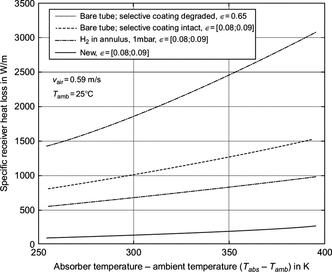
The first step in performance and acceptance testing is to identify the model parameters describing the optical, angular and thermal dependency of collector performance, see Fig. 7.14 lower part. To this end, the mass flow rate, inlet and outlet temperatures, and the DNI have to be measured. Moreover, the solar field operating conditions, such as mirror cleanliness or the tracking modus of the collector (totally or partly focused, described by ffocus), ambient conditions such as temperature and wind, and the specific heat capacity of the heat transfer fluid must be known or measured. The field efficiency for parabolic troughs can be measured using Eq. (7.15) [61, 62]:

The symbol χ represents the mirror cleanliness derived by reflectivity measurements. It is assumed that the receiver glass envelope is soiled likewise. In a second step (see Fig. 7.14 upper part), the performance parameters are used to calculate the annual energy yield for given solar irradiation and ambient conditions.
Quasi-steady-state, e.g. [62], and quasi-dynamic methods, e.g. [63,64], have been frequently used in the last years. Dynamic models in contrast to quasi-dynamic models have the advantage that both the inlet temperature as the mass flow rate can be varied during testing. Hence, they enable to include warm-up and cool-down periods in the parameter identification process, which reduces the number of necessary test days. A good comparison between the quasi-dynamic and dynamic method is presented in [64] by applying both methods to a linear Fresnel collector. Janotte [65] compares results of quasi-steady-state methods with dynamic methods and states that, thanks to the broader acceptable temperature range during morning heat-up and night cool-down, dynamic methods can better decouple the identification of correlated parameters, hence increasing robustness of the process. Good experience is reported for the dynamic method characterizing a modern large-aperture collector demonstration loop. A comprehensive literature overview of the different performance evaluation methods and a survey about dynamic evaluation procedures is found in Ref. [66].
The parameterized dynamic performance model (PDPM) for parabolic troughs as presented in [60,61] is a simplified dynamic model which overcomes the limitations of the quasi-dynamic modeling approach. It is not a detailed dynamic model as described in e.g. [67,68], because this would involve many more parameters and consequently complicate parameter identification. Instead, the collector or loop performance is based on a quasidynamic collector performance equation including a heat capacity term (Eqs. 7.16–7.19), which is coupled to a large number of cascading continuously stirred tank reactor models. The continuously stirred tank reactor modules simulate residence time effects, varying flow rates, and mixing effects of the fluid flow. The collector heat gain is

with ffocus being the collector focusing factor, the incidence angle modifier (IAM) κ(θ) defined as a function of the incidence angle
the mean fluid temperature being
and the difference of mean fluid temperature to ambient being
The parameters of interest identified with the measured heat flow are the optical efficiency ηopt, the IAM coefficients a1, a2, the thermal loss coefficients c1, c2, and the specific heat capacity coefficient ccap. Usually, 5–10 sunny test days, representing all seasons of the year, are needed to estimate the parameters. The dynamic approach is not limited to this equation; other formulations are possible.
Fig. 7.15 shows exemplarily the measured and modeled heat gain of a Skal-ET collector loop over almost 7 h of a day. The dataset presented has not been used for parameter identification. The deviation of measured and modeled heat gain is also shown with the continuous red line. Changes in heat flow rate caused both by variations in direct solar irradiation as by variation of the mass flow rate are simulated with good accuracy. The deviation in integral energy gained over the plotted period is in the range of about 0.4% only.

The approach of a parameterized dynamic performance model (PDPM) can also be applied to solar fields or subfields by condensing all parallel loops into one average loop and representing the characteristics of the header pipes by few cascading continuously stirred tank reactors. As a consequence, the result is an overall (sub)field performance characteristic, which allows the determination of the thermal output of the complete (sub)field. This is sufficient if in acceptance testing, the performance of the whole field is agreed upon between the parties.
Other systems require adapted underlying performance equations. Dynamic models for linear Fresnel systems are described in e.g. [64,69]. Due to their fixed receiver, linear Fresnel collectors need a two-dimensional IAM function (longitudinal and transversal component). Discretization of the receiver flow is realized in Ref. [64] as a multinode model.
A high measurement accuracy of the measurement instruments is crucial for successful parameter identification. Refs. [61,62] study the influence of instruments on the uncertainty of performance data. A good overview of possible measurement approaches is listed in a best practice guideline [70]. Standard plant instrumentation may have least costs and effort, but usually does not have sufficient measurement accuracy. Plant instrumentation can be upgraded with calibrated sensor to increase accuracy. Alternatively, a mobile heat unit with calibrated instrumentation could be connected. Another possibility is to foresee flanges in the collector piping to connect a bypass with a highly accurate Coriolis sensor, embedded PT-100, and an online flow-through calorimeter for specific heat capacity measurement [10,71]. Less interference with the plant operation and leakage risk can be achieved by employing a mobile field laboratory with “clamp-on” sensors for temperature and mass flow rate. Recent advances further reduced uncertainties of clamp-on temperature measurement techniques. Applying a correction, the uncertainty is only doubled compared to wetted sensors, being below ±0.6 K for up to 390°C. Clamp-on ultrasonic sensors which are thermally decoupled from the tube by a wave-injector show an uncertainty in mass flow rate of approximately 1.4% for thermal oil during tests.
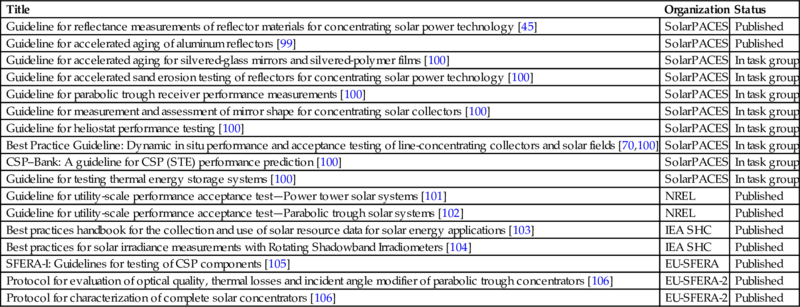
Currently, a best practice guideline [70] regarding performance and acceptance testing of line-concentrating collectors and solar fields is in the international discussion phase as part of the SolarPACES-Task I activities.
7.2.3 Airborne measurement of optical system performance
Due to the different optics, optical measurement techniques based on deflectometry or fringe reflection to qualify the performance of line-focusing technologies, such as parabolic troughs or Fresnel collectors, differ from techniques of heliostats of a central receiver system. In central receiver systems, a single, stationary mounted camera on the tower top can take images of all heliostats for deflectometric evaluation. For this reason, automated systems to measure the slope deviations of heliostats of central receiver systems are already offered commercially (see Chapter 5). For line-focusing collectors, the camera has to be manually positioned and moved from collector to collector, and often the distance between adjacent rows is not sufficient to have the necessary distance to the collector making necessary lifting platforms.
Therefore, image acquisition is time consuming and applicable to only small fractions of the solar field. Other measures like torsion characterization rely on inclinometers with their high effort for installation and data acquisition. The measurement volume is limited despite advanced optimization of all processes and the effort during evaluation is comparatively high.
Recently, the use of unmanned aerial vehicles (UAVs) for image acquisition tasks has gained much attention. Colomina [72] presents a comprehensive overview on civil remote sensing applications of UAVs. In the renewable energy area, UAVs are used to monitor wind turbines [73] and photovoltaic installations [74]. Jorgensen [75] was the first one to assess the potential of the airborne implementation of the distant observer method [76] and IR camera based receiver tube characterization to large parabolic trough collector fields. A first implementation of this approach has been described in Ref. [77,78].
The airborne measurement system of DLR, called QFly [77], is developed to obtain the optical performance for entire parabolic trough fields. Fig. 7.16 shows the workflow of QFly. The system consists of a commercially available quadcopter and software code for pre-flight route planning and postflight evaluation from raw images to spatially resolved slope deviation information and receiver position. It is coupled to raytracers, which enable the automatic output of intercept factors.

The system is based on the Trough Absorber Reflection Measurement System (TARMES, [79], see Chapter 5), which uses the edges of the reflection of absorber tube in the collector mirrors. This includes fully automated airborne determination of the absorber tube position relative to the focal line with a photogrammetric approach and subsequent calculation of the mirror slope in curvature direction from the reflection of the absorber in the mirror. A basis for accurate results is a postflight determination of the camera position relative to the solar field. This task is performed via close range photogrammetry [80] using artificial markers and collector features like mirror corners as point of interest; see Fig. 7.17. An iterative bundle-adjustment enables simultaneous calibration of the inner orientation of the camera and delivers 3D coordinates of the mirror corners and positions and camera orientation (3D location coordinates and angles) for each image. Overall accuracy for spatial coordinates has been estimated to approx. 5 mm via cross checking with a total station and back-projection of the features in the images [77]. Using this information, an orthoimage as shown in Fig. 7.18 is created, from which the absorber tube reflection can be derived.


The automatic flight route incorporates a rising and descending path to each collector module fly-over in order to obtain perspectives for absorber tube positioning, while during the horizontal part of the route images are taken to derive the slope information; see Fig. 7.19.

Measurement uncertainty has been cross-checked with independent close range photogrammetry measurements. It is in the range between ±0.6 and ±1.1 mrad for the local slope deviation and ±1.5 mm for the absorber tube position. Fig. 7.20 shows a typical slope deviation map of a collector module.

The QFly system is currently capable to perform the data acquisition for two 150 m long EuroTrough-type collectors within 60 min and automatic data post processing within 2 h. The approach presented here delivers high-resolution geometric information of a parabolic trough collector, but has limited measurement capacity due to actual flight time restrictions and maximum frame rates of the camera. With the current setup (Camera SonyNex7: frame rate below 2 fps, UAV Microdrones MD4-1000: flight time below 45 min), about two loops per day could be characterized under ideal conditions.
Although future camera and UAV developments will increase this measurement volume, a modified “survey” approach is currently under development to characterize an entire solar field for a plant with turbine output of 50 MWel and a 7.5 h thermal storage in less than 1 day. With altitudes in the range between 100 and 250 m, the entire field is scanned with a few east-west straight fly-overs while continuously acquiring images. One image is shown in Fig. 7.21. The absorber tube reflection is considerably larger compared to the low-altitude flights. Absorber tube positions can currently not be derived at these flight heights and angles of observations. As a consequence, only “effective” slope deviations and results in lower resolution can be derived. “Effective” slope deviation results are not corrected for any possible misalignment of the absorber tube and are a combination of physical mirror slope deviations and absorber tube misalignment. However, having various modules in one image, tracking deviations and any module misalignment or torsion information inside a collector can be obtained.

The survey mode can be applied when the collector evaluation is close to zenith ±10° and aims to deliver results for the tracking deviation even under full illumination of the absorber while the field is in tracking mode with high solar irradiance values. The main difference to low-altitude flights is the methodology to estimate the camera position. Solar field features are projected back into the photo and the residuals between projected and detected features are minimized by varying the camera exterior orientation.
Replacing the visual camera with a long-wavelength infrared camera (e.g., FLIR Tau 640) offers the possibility to measure the glass envelope tube temperature of the receiver. A high glass envelope temperature of a receiver in a fast airborne infrared screening indicates defective receivers which may be studied in details with the technique presented in section 7.1.2.
NREL has a long track record concerning UAV based qualification of solar fields [75]. Theoretical investigations have been made concerning qualitative and quantitative evaluation of mirror and receiver geometry, IR measurements of receivers, and airborne vehicles. The mirror and receiver geometry is derived with a photogrammetric method. Camera positions are determined using artificial markers which have to be deployed on the collectors. The mirror slope is derived from the photos by using the center line of the receiver tube reflection. Similar accuracies as reported above are reached [78].
It is planned to extend the capabilities of the presented airborne image acquisition technique and software modules as fast and comprehensive qualification methods to linear Fresnel collectors and determination of heliostat offsets in the future.
7.2.4 Rotating platforms for line-focusing collectors
One-axis tracking systems per definition are not able to follow the sun in a way that all sun rays hit the collector aperture perpendicularly. For east-west oriented parabolic troughs, perpendicular incidence only occurs once at noon. For north-south oriented collectors, it may never occur or only during the summer at a specific point in time. Linear Fresnel systems, as they have fixed receivers, have two incidence angle components: the transversal (which is zero for troughs) and the longitudinal. The IAM describes the optical behavior of a collector with oblique incidence angles compared to a situation with perpendicular incidence. With perpendicular incidence, the peak optical efficiency is reached, which is an important parameter for collector qualification.
To characterize real-size collectors in on-sun tests, it is convenient to be able to adjust any incidence angle at any time desired. For this reason, different rotating platforms for line-focusing collectors have been developed and constructed [3,81–84]; see Fig. 7.22. They offer perfect conditions for the thermal and optical qualification of real-size collector modules in outdoor conditions, including mirrors and receivers, for the development of standards, and to demonstrate on-sun the functionality of industrial components and systems.
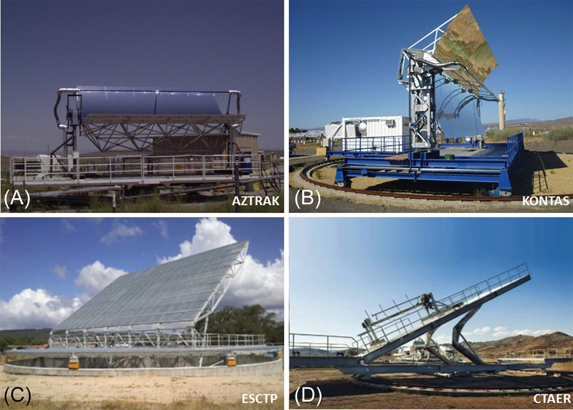
The AZTRAK and KONTAS are azimuth tracking platforms which are designed for parabolic trough modules with their own elevation tracking system. The ESCTP and CTAER platform are azimuth and elevation tracking platforms which can also bear other collectors, e.g., linear Fresnel collectors. More information is listed in Table 7.3. In addition to these platforms, NREL has a large-payload two-axis solar tracker which can support different collectors. Parabolic troughs up to 16 m can be mounted on the tracker. The system does not have its own balance of plant [85].
Table 7.3
Overview of existing rotating platforms
| AZTRAK [81,82] | KONTAS [3] | ESCTP [83] | CTAER [84] | |
| Institution | Sandia National Laboratories | DLR-CIEMAT (PSA) | University of Évora | CTAER |
| Description | Azimuth tracking platform for parabolic troughs | Azimuth tracking platform for parabolic troughs (actual: Skal-ET) | Azimuth and elevation tracking platform for parabolic trough and linear Fresnel | Azimuth and elevation tracking platform for parabolic trough and linear Fresnel |
| Tracking range | Azimuth: ±115° | Azimuth: ±170° | Azimuth: ±170° Elevation: 0–40° | Azimuth: ±120° Elevation: 0–37° |
| Length/width | <13 m length | <20 m length | <18 m length, <13 m width | <24 m length, <15 m width |
| Fluid | Syltherm 800 or water | Syltherm 800 | Syltherm 800 | Syltherm 800 |
| Temperature range | 50–400°C | Ambient to 400°C | 12–385°C | up to 400°C |
| Inlet temp. stability | ±0.2 K | ±1 K | n/s | ±1 K |
| Temperature measurement | 4-wire PT-100 at inlet and outlet | 3 simultaneously calibrated 4-wire PT-100 each at inlet and outlet, upstream mixer | 4-wire PT-100 at inlet and outlet | n/s |
| Balance of plant | Electric heater (40 kW), water cooling | Heating and cooling unit (100 kW) | Heating (53 kW) and cooling unit (156 kW) | Heating and cooling unit (with step change up to 100°C for aging) |
| Mass flow sensor | Two turbine flow meters | Coriolis sensor: DT 150H 0.53–6 kg/s | Coriolis sensor | n/s |
| Specific heat capacity | Data sheet | Measurable by a flow-through calorimetera | Flow-through calorimeter planned | Data sheet |
| Measurement uncertainty for total efficiency | ±2% to ±5% | ±2% to ±3% | n/s | n/s |

a The flow-through calorimeter [10] has an uncertainty of 1.0% [71].
The most important tests performed are as follows:
• Total peak efficiency of collector assembly (including receivers) at normal incidence and at different temperatures, derived with hot on-sun tests. In addition, the total efficiency under non-normal incidence can be derived.
• Optical peak efficiency of collector assembly (including receivers) at normal incidence, derived with cold on-sun tests. Additionally, the optical efficiency of a collector assembly (including receivers) at non-normal incidence can be measured with cold on-sun tests to determine the IAM. Caution has to be taken that the IAM of a collector differs from that of a collector module due to the end losses.
• Receiver thermal loss at several temperatures, derived with hot tests without sun at night (clear sky). Special care has to be taken not to “radiate” the receivers by clouds or warm surroundings or to apply corrective terms.
7.3 Durability assessment
7.3.1 Overheating and thermal cycling of parabolic trough receivers
Accelerated aging of parabolic trough receivers is an important means to assure the performance over the lifetime and time of warranty. Absorber coatings have to withstand operating temperatures around 400°C for thermal oil plants and above 550°C for direct steam or solar salt plants. An accelerated test to check whether a coating can withstand extended times at these temperatures is to overheat the coating, e.g. [86].
Carlsson [87] describes the method used for collectors for domestic hot water systems. It is assumed that the degradation of the coating can be described by the Arrhenius equation. The reaction rate k of the degradation processes, that can be chemical reactions or diffusion, depend exponentially on temperature T (in K) [88, p. 257] by
where R is the ideal gas constant. Characteristic for the degradation process are the constant A and the activation energy Ea. Assuming an equal number of reactions for the same aging result, a test performed at temperature Ttest for the time ttest simulates the aging of the receiver in the solar field that was exposed to temperature Tsim for the time tsim. The time for the test ttest can be calculated using Eq. (7.21):

It can be seen from Eq. (7.21), that the constant A present in Eq. (7.20) disappears in Eq. (7.21). The activation energy Ea, on the other hand, needs to be known before the test. It can be determined by performing accelerated aging tests at different temperatures and evaluating Eq. (7.20).
For aging tests of small absorber samples, the change in absorptance α and emittance ϵ determined with spectrophotometers is the main information of interest. Other analysis techniques can be useful in coating development. Cachafeiro et al. [86], for example, investigate the coating before and after accelerated aging by Glow Discharge Optical Emission Spectroscopy.
Manufacturer-independent qualification laboratories often prefer to test entire receivers instead of small absorber samples. Overheating of an entire receiver is achieved using heating cartridges or direct Joule heating similarly to heat loss testing described in Chapter 4. As temperatures are usually measured with thermocouples, the systematic temperature measurement errors and their correction need to be addressed. Accelerated aging of entire receivers is relatively expensive. Hence Pernpeintner et al. [89] proposed not to determine testing time according to Eq. (7.21), but to apply the same testing conditions to all receivers under consideration to simplify testing. As the activation energy Ea is not determined in this case, lifetime predictions cannot be achieved.
The proposed testing time is 1000 h [89]. The proposed testing temperature was to be determined from the maximum operating temperature in K Tmax,K using
This yields a testing temperature of Ttest,K of 478°C for receivers to be used with thermal oil having a maximum temperature of 400°C. First tests furthermore showed the usefulness of limiting the heat-up rate to 5 K/min. Additionally, at first heat-up of the receiver above 400°C, a three step heat-up procedure is followed. Below 400°C, heat-up is limited to 5 K/min, at 400°C the temperature is maintained constant for 24 h, and above 400°C the heat-up-rate is limited to 0.05 K/min.
With the availability of automated test benches for overheating, additional aging tests can be conceived. Hence, Pernpeintner et al. [89] propose performing thermal cycling tests on receivers from 200°C to the overheating temperature calculated according to Eq. (7.22). Cooling down is achieved by switching off the power. 100 cycles times are proposed in Ref. [89] that take about 3 weeks to complete in a setup with heating rods and without active cooling. The heat-up rate is again limited to 5 K/min.
7.3.2 Durability testing of glass-to-metal seal and bellow of parabolic trough receivers
The glass-to-metal seal and the bellows are important parts of the receiver which are at the risk of failure. The glass-to-metal seal connects the brittle glass material to a metal with typically rather different thermal expansion coefficients. Hence, temperature differences lead to thermal stresses in this component. The bellow, on the other hand, is compressed and expanded approximately 10,000 times within the projected lifetime of the receiver. Both the glass-to-metal seal and the bellow must maintain their airtightness over the lifetime of the receiver.
Chiarappa [90] presented a test bench for the accelerated aging of the glass-to-metal seal. The test bench does not test an entire receiver, but an assembly of glass tube, glass-to-metal seal, and bellow. In the test bench, a collar with infrared heating elements surrounds the glass-to-metal seal. In a test, the temperature at the glass-to-metal seal is varied from 20 to 250°C. Additionally, a mechanism applies axial forces on the assembly that lead to a length change in bellow of up to 22 mm. During the test, the helium leak rate is observed.
Pernpeintner [89] presented a test bench for the testing of entire receivers, which simulates the mechanical and thermal stresses on the bellow; see Fig.7.23.

Using a heating rod similar to those used in heat loss testing and receiver overheating, the absorber is heated to half the temperature between room temperature and operating temperature, typically 200°C in order to create half the absorber extension. The absorber tube is then fixed and the glass envelope is pushed back and forth using an envelope clamp and a system of motor, eccentric shaft, and a push-pull shaft. A counterweight compensates for the weight of the envelope clamp so that the bellows carry merely the weight of the glass envelope during the test. The movement is operated at 1 Hz. A typical test performs 20,000 cycles followed by a 24-h waiting period. A total of 20,000 cycles correspond to approximately 50 years of field operation, assuming one cycle per day. The waiting period of 24 h is used because small leakage rates require some build-up time to manifest in increased heat loss. During the whole test, the heating power is monitored as it indicates any possible leakage.
7.3.3 Durability testing of receiver materials for solar towers
Receiver materials used in solar thermal power tower plants are typically exposed to far higher temperatures than parabolic trough receivers. Volumetric receivers, for example, can heat gases to temperatures over 1000°C [91–93]. They are used to drive gas turbines, chemical processes, or to generate steam. Tubular metal receivers heat molten salt to produce steam for Rankine [94] or supercritical cycles, or preheat air for Brayton cycles [58,91], for example. High absorption coatings on these tubular metal receivers frequently have to withstand temperatures as high as 750°C and high UV radiation. The tube material has to be corrosion resistant to the heat transfer medium, while being subject to thermal cycling and mechanical stress.
The subject of durability testing of receiver materials for solar towers is broad and currently strongly developing. This section exemplarily presents two examples for durability testing. Testing is frequently conducted on a smaller scale, such as a dish concentrator or a solar furnace instead of a real-scale solar tower.
7.3.3.1 Durability testing of volumetric silicon carbide receivers of solar towers
The open volumetric receiver technology HiTRec (High Temperature Receiver) [93,95–97] aims at generating hot air which can be stored in a recuperative storage or directly used to generate steam and drive a turbine. The receiver consists of modular ceramic silicon carbide (SiC) absorber cups with numerous parallel channels. A blower behind the receiver is used to suck ambient air through the ceramic channels. The air is heated up to 800°C while flowing through the ceramic cups. Because the maximum temperature is reached inside the volumetric absorber structure, heat radiation losses on the front surface are reduced significantly. An average efficiency of 74% has been measured for a 3 MW-receiver at 700°C. Theoretically, higher efficiencies of more than 90% are possible.
The main failure mechanism observed in SiC honeycombs is cracking due to thermal stresses, after around 1500 h. When a cloud rapidly shadows the heliostat field of the solar tower while the absorber is at its working temperature, it cools down with up to 500 K/min. Similar to flux gradients on the receiver surface, these transients also produce high material stresses and provoke cracks or even breaking of the material.
Thermal cycling tests of volumetric receiver cups should be conducted with a solar concentrator that simulates the typical operation conditions. The test bench should measure and control the air temperature at the receiver outlet (200?–800°C), air mass flow (0.010?–0.020 kg/s) and return air temperature (100–200°C). It should allow an easy positioning of the receiver relative to the focal point, a remote control, and automatic data logging.
Dish concentrators have been used for this purpose before. Fig. 7.24 shows the test bench which is in use on the Plataforma Solar de Almería (PSA).

The concept of this test bench is illustrated in Fig. 7.25. The main air path consists of the open volumetric air receiver, a tube and a heat resistant air blower. The inbound ambient air is heated up in the receiver, flows through the inner tube, and exits through the main blower into the environment. The receiver cup outlet temperature (Trec,out) and mass flow (![]() ) are measured in the tube. The receiver outlet is controlled by the rotation speed of the blower.
) are measured in the tube. The receiver outlet is controlled by the rotation speed of the blower.

A second tube with bigger diameter covers the inner tube to simulate the return air of the volumetric receiver concept. The return air, which is cold ambient air conveyed by a second blower, flows through the gap between the tubes in the reverse direction and heats up to the desired temperature by heat exchange with the hot inner tube. At the same time the inner air flow is cooled and material stress reduced. The return temperature is measured just before it leaves through the gap between the absorber cup and the box, which encloses the cup. Here the air temperature also is controlled by the blower speed. If no return air is desired, the mechanical slide valve in the annular gap can be closed and the slide valve on the surface of the outer tube opened, so the return air keeps cooling the inner tube. Testing without return air provokes higher thermal gradients and material stress, and can be considered the worst case.
The following procedure is followed to test the cracking resistance:
• The mass flow of air flowing through the tested SiC honeycomb is 0.015±0.005 kg/s.
• The temperature of the air stream is directly measured behind the absorber cup. At least three thermocouples should be employed and the mean temperature should be considered.
• The air stream is heated up to 750±20°C. After reaching the maximum temperature, the air should be cooled down to 200±20°C.
• The sample should be heated and cooled down for 15 times, being the heating and cooling rate of the air (250±50)K/min.
• A secondary air stream of 150±50°C with no specified mass flow shall circulate around the absorber cup in opposite direction from the main air flow to simulate the recirculation in power towers.
• The flux gradient on the front surface of the tested specimen should be smaller than 40 kW/m2/cm. This value is approximately 10 times higher than flux gradients appearing in a 1-MW solar power tower.
Fig. 7.26 shows an example of the measured cup outlet temperature, temperature gradient, return air temperature, and DNI of part of a typical thermal cycling test.

Fig. 7.27 shows the measured cup outlet temperature, the temperature gradient, and a microphone signal of the test performed with the cup shown in Fig. 7.24. The microphone is located behind the front protection, close to the absorber cup. The cracking of the material usually emits a loud sound, which can be recorded with a microphone. In this way, the exact point in time of breakage can be determined. The particular sample under examination cracked at a thermal gradient of 300 K/min.
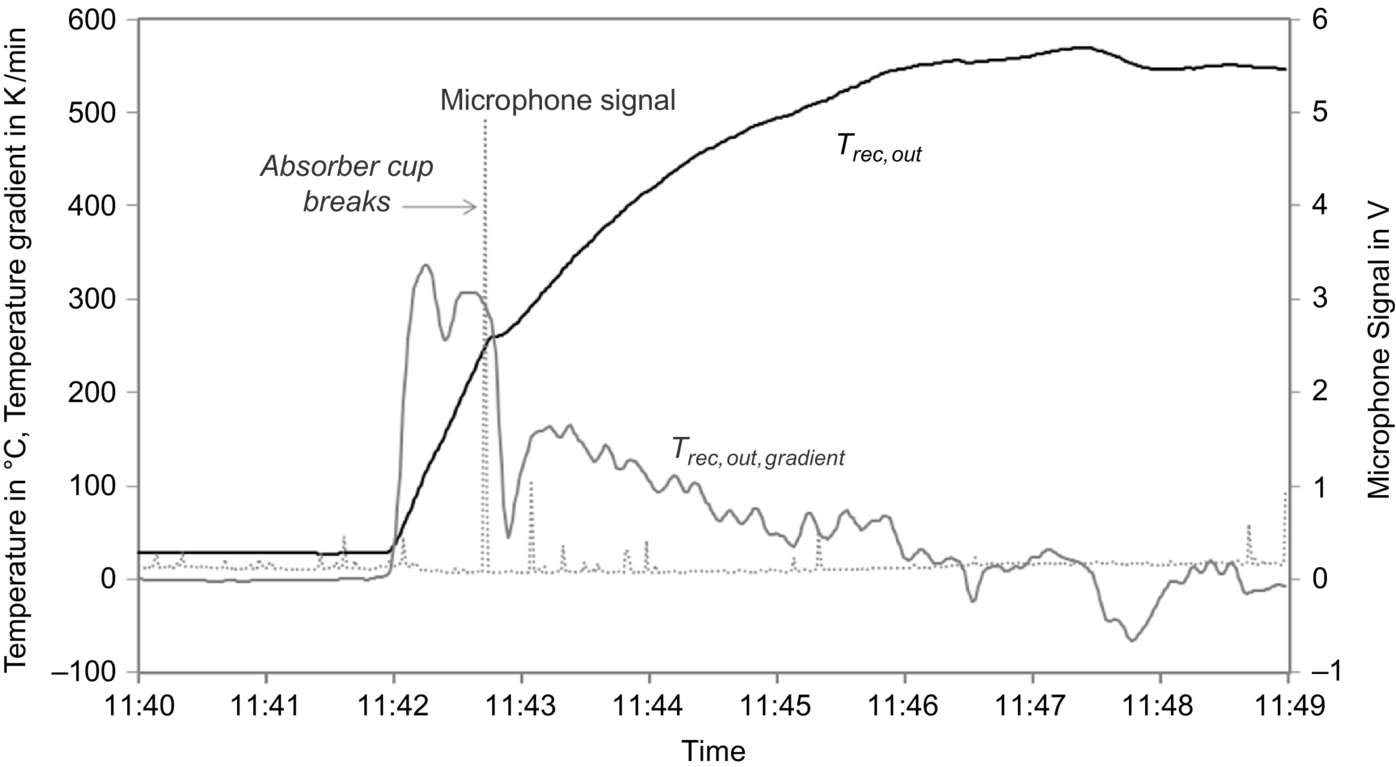
7.3.3.2 Durability testing of coatings for tubular receivers
Coatings with high solar absorptance and coatings with selective properties stable in air combined with a long service lifetime are being developed. A test bench has been erected on the Plataforma Solar de Almería on a dish concentrator to test the durability of uncoated and coated tube samples to be used in a tubular receiver [98]. Currently, the test bench is further optimized to maintain a desired level of solar flux, while controlling the temperature. Defined heating and cooling gradients should be applied to allow a controlled thermal cycling testing. An automated positioning table combined with an air convection cooling system is used to control temperature and solar radiation. The samples are examined for any changes in optical properties, or mechanical failure.
7.4 New guidelines and standards under development
Different activities targeting the establishment of standards are currently being followed. They have varying maturity and are pursued on different levels (national, bi-national, international). Usually, scientific platforms like SolarPACES or in the framework of national or European cooperation projects, first protocols or guidelines are developed and discussed. At the same time, standardization organizations work in their respective working groups on standards, ideally taking into consideration the protocols and guidelines of the scientific platforms. This section gives (without any claim to completeness) a list of activities of standardization organizations (Table 7.4) and scientific platforms (Table 7.5) regarding guidelines and standards under development.
Table 7.4
Activities of standardization organizations regarding guidelines and standards.
| Title | Organization | Status |
| International Electrotechnical Commission IEC TC-117 “Solar Thermal Electric Plants” | IEC | Unpublished |
| Spanish Association for Standardisation and Certification AEN/CTN 206/SC117 “Thermoelectric Solar Energy Systems” | AENOR | Unpublished |
| American Society of Mechanical Engineers ASME PTC-52 “Concentrating solar power plants”, ASME PTC-53 “Mechanical and thermal energy storage” | ASME | Unpublished |
Table 7.5
Activities of scientific platforms regarding guidelines and protocols.
| Title | Organization | Status |
| Guideline for reflectance measurements of reflector materials for concentrating solar power technology [45] | SolarPACES | Published |
| Guideline for accelerated aging of aluminum reflectors [99] | SolarPACES | Published |
| Guideline for accelerated aging for silvered-glass mirrors and silvered-polymer films [100] | SolarPACES | In task group |
| Guideline for accelerated sand erosion testing of reflectors for concentrating solar power technology [100] | SolarPACES | In task group |
| Guideline for parabolic trough receiver performance measurements [100] | SolarPACES | In task group |
| Guideline for measurement and assessment of mirror shape for concentrating solar collectors [100] | SolarPACES | In task group |
| Guideline for heliostat performance testing [100] | SolarPACES | In task group |
| Best Practice Guideline: Dynamic in situ performance and acceptance testing of line-concentrating collectors and solar fields [70,100] | SolarPACES | In task group |
| CSP–Bank: A guideline for CSP (STE) performance prediction [100] | SolarPACES | In task group |
| Guideline for testing thermal energy storage systems [100] | SolarPACES | In task group |
| Guideline for utility-scale performance acceptance test—Power tower solar systems [101] | NREL | Published |
| Guideline for utility-scale performance acceptance test—Parabolic trough solar systems [102] | NREL | Published |
| Best practices handbook for the collection and use of solar resource data for solar energy applications [103] | IEA SHC | Published |
| Best practices for solar irradiance measurements with Rotating Shadowband Irradiometers [104] | IEA SHC | Published |
| SFERA-I: Guidelines for testing of CSP components [105] | EU-SFERA | Published |
| Protocol for evaluation of optical quality, thermal losses and incident angle modifier of parabolic trough concentrators [106] | EU-SFERA-2 | Published |
| Protocol for characterization of complete solar concentrators [106] | EU-SFERA-2 | Published |