
Methods to provide meteorological forecasts for optimum CSP system operations
M. Schroedter-Homscheidt*; S. Wilbert† * German Aerospace Center (DLR), Oberpfaffenhofen, Germany
† German Aerospace Center (DLR), Almería, Spain
Abstract
Having seen that meteorological forecasts of DNI may help in performance assessment in CSP systems, this chapter provides an overview on DNI forecast options. Nowcasting for the upcoming few hours and forecasting for the upcoming days is treated separately. The chapter provides an introduction in meteorological basics and terminology being useful for the reader when ordering forecasts from operational meteorological centers or meteorological service providers. After that the technologies based on numerical weather prediction, statistical time series modeling, all-sky imagers, and satellites are described. Necessary postprocessing steps to be performed after obtaining the standard weather service products are discussed as well. After reading this chapter, an engineer should be capable of understanding what kinds of forecasts are routinely provided, what each forecast includes and how to use them properly.
Keywords
Nowcasting; Forecasting; Numerical weather prediction; Statistical time series models; All-sky imagers; Satellites; Meteorological basics; Routine meteorological forecasts
8.1 Introduction
The planning, engineering, and financing of concentrating solar power (CSP) plants requires solar resource information based on long-term historical databases. The operation of CSP plants requires knowledge on a wider range of the upcoming meteorological conditions. Obviously, there is the need for forecasting direct normal irradiation (DNI), but in addition to this, other meteorological parameters as air temperature, humidity, wind speed, and wind gust speed are needed.
After defining meteorological terminology in Chapter 8.1.1, we focus on forecast verification strategies in Chapter 8.1.2. Chapters 8.2 and 8.3 deal with the forecasting and nowcasting of irradiances, while Chapter 8.4 discusses developments to be expected in the future.
8.1.1 Meteorological definitions
The forecast horizon or forecast length is the number of minutes, hours, days, or months up to which a forecasting system delivers predictions. In meteorology, very short-term forecasts provide forecasts up to 12 hours; short-term forecast is defined from 12 to 48, 60, or 72 hours; medium-term forecasts are defined as up to 10–14 days (240–336 hours), and long-term forecasts cover monthly or seasonal predictions. Below the forecast horizon of very short-term forecasts, there is a shorter forecast horizon called nowcasting or sometimes also extremely short-term forecasting. Originally, the World Meteorological Organization [1] defined the forecast up to 2 hours as nowcasting, but nowadays, meteorologists typically define nowcasting as the forecast up to 6 hours.
In the energy sector, the nowcasting range is also called short-term forecasting while long-term forecasting is meant as a forecast for several days and very short-term forecasting is defined as up to 30 minutes. The origin of this wording is based on the typical forecast horizons used in electricity grid operations: intrahour for the second to minute range below 60 minutes, intraday for a few hours, and intraweek for a few days ahead forecasts. The energy sector tends to use the meteorological terminology very short term, short term, and long term as synonyms for intrahour, intraday, and intraweek, which causes continuous confusion and misunderstandings. Therefore, we suggest keeping the terminology intrahour, intraday, and intraweek as wordings in the energy sector and keeping nowcasting, very short-term, short-term, and medium-term forecast horizons as meteorological terms (Fig. 8.1).

Terminology as forecast lead time or temporal resolution are visualized in Fig. 8.2 and discussed in the following section. Forecast lead time is the time difference between the start of the forecast and the occurrence of a forecasted value. In the case of a forecast initialization at 13:00 UTC and a forecast value for 13:45, the forecast lead time is 45 minutes. It is a proper name for the x-axis if plotting a DNI forecast over time until, e.g., the forecast horizon.

For all applications discussed here, the required DNI values represent an accumulated value over a certain time interval. The forecast temporal resolution defines the length of these time intervals. A temporal resolution of 15 minutes means that forecasted values are provided for the lead time intervals 1–15, 16–30, 31–45 minutes, etc. It is important for the forecast system to represent the average over the time interval and not just an instantaneous value at a particular moment. Please note that in numerical weather prediction (NWP), the output is typically given as an accumulated value over a period of time in J/m2 and that the time stamp is given at the end of the time interval.
The refresh rate of the forecast is defined as the frequency the forecast system is started again and the prediction values are updated. It may be 6 hours as typical for global-scale NWP and down to a few minutes for statistical approaches in short-term forecasts.
Typically, a time lag between the start of a forecast run and the availability of the forecasted values exists. Mainly this is caused by the need to wait for observations being delivered to the NWP center in order to be assimilated. Often a symmetric time around the nominal start time of the forecast run is chosen as the acceptance window for ground observations. Only after the end of that time window, the forecast system can run. Additional reasons are significant processing times or spin-up times. Spin-up is a process in numerical parameterizations which ensures adjustment of the model to the actual boundary conditions. Finally, the forecast will start at the nominal start time of the run, even if actual wall clock time may be already 1 or 2 hours later. Only some time later the forecast run will have reached the actual wall clock time and starts providing any forecast.
Point forecasts provide a time series of forecasted DNI values being valid for a geographical point, most likely being defined by a geographical latitude and longitude. Gridded forecasts provide several time series being valid for a numerical grid point each, e.g., at regularly distributed locations, being defined by their geographical latitude and longitude. Grids may be regularly distributed in latitude and longitude, but most meteorological grids in NWP are not, in order to cope with the heterogeneous distance between latitudes and longitudes on the Earth sphere. Meteorological service providers may re-grid NWP model output to allow a regular gridded output being provided to users from the non-meteorological sector. Gridded forecasts allow visualization as a video of DNI values in a geographical map allowing an intuitive forecast assessment by a power plant operator. It should be noted that gridded forecasts represent a grid box average and therefore a spatial average.
Besides using a single DNI value or a single DNI spatial map per time step from a deterministic forecast, weather forecasting may also provide probabilistic information as the probability density function of an event occurring. Such an event may be the exceedance of a certain DNI value at a point in time and space.
With respect to the assessment of forecast accuracy, one can either evaluate the most recent forecasts or evaluate historical forecasts being made earlier and stored as they have been made. If evaluating most recent forecasts, near real-time observations need to be made available. If evaluating historical forecasts, historical observations can also be used. This allows a more lengthy collection and quality control of observations. However, it also requires the storing of already made forecasts without any changes. National meteorological services typically store their forecasts for long-term access also due to internal development requirements. For commercial meteorological service providers, this may not always be feasible or automatically foreseen.
This approach has to be separated from so-called reanalysis datasets. In a reanalysis project, a meteorological service re-runs historical forecasts, but based on a more recent model version. This provides a consistent set of forecasts with respect to model physics. It may be more appropriate to use such a reanalysis in order to assess longer time periods with their natural variability of the atmosphere, but with the same and more recent model physics representation. In the case of strongly varying model physics from version to version during time, this may be more appropriate to assess the forecast quality of the nowadays existing forecasting system.
There are some potential drawbacks. Often reanalysis projects are performed on a lower spatial resolution. This will change evaluation results as especially clouds are small-scale dependent phenomena. And depending on the priority of the reanalysis project, the duration of an observation data assimilation window may be different from the operational forecast configuration. In the case of a longer observation window, the situation is quite different from the operational use of the forecasting system. In such a model configuration, the model has much more insight in the atmospheric state than it does have in the operational configuration. Both cases may block the use of reanalysis data for the assessment of nowadays forecast capabilities. However, if this is not the case, any reanalysis program is of great use.
Finally, a short note about hindcasting: this is a method to run a forecasting system for past times, but without making use of extended observations as is done in, e.g., a reanalysis project.
8.1.2 Forecast verification
Comparing any numerical model based forecasts versus the measured “truth” or reference is called forecast verification in the meteorological sector. This is frequently called validation, but this is wrong in the strict sense. Validation generally requires knowledge of the “truth” based on independent measurements (also called observations) of the same physical quantity or phenomenon. Additionally, validation should be based on repeated observations. In the atmosphere such a repetition of the same observation is not available, as the atmospheric state is variable in time and space.
Additionally, each measurement system observes another volume of the air than the forecast is valid for. A forecast is always valid as a mean over a grid box volume or over a satellite pixel area. For satellite pixels, the column between the observed surface and the satellite optics is always measured as a whole. The same applies, e.g., for a DNI measurement which always has a nonzero sensor size and is probing the volume in its field of view. Also, any wind speed observation is probing an air volume of some spatial extension. Generally, it lacks the spatial representativeness for the pixel or NWP grid box being evaluated. Therefore, the term validation is avoided and replaced by words like comparison, evaluation, or verification. Please note, this is not consistent with a definition used, e.g., in informatics where verification asks whether a numerical software code reproduces any conceptual model like a physical equation sufficiently well and validation asks for the suitability of the numerical software output versus observations including all extreme cases in the application of the software.
Forecast verification is a process to assess the quality of a forecast. It may not represent the value of a forecast. A forecast has value if it helps the user to make a better decision compared to an easily accessible forecast, e.g., persistence, chance, or climatology. This decision may be based on, e.g., economical or security considerations. The user's cost-loss function is very specific and may represent the electricity market conditions. Costs in this case mean the costs of a forecast, while loss is the potential loss due to any wrong forecast. Alternatively, it may be defined by any power purchase agreement details, or by thresholds of minimum required DNI values for start-up procedures or maximum wind speed values for security reasons. Therefore, the relevance of specific forecast events may be much higher than other forecast situations. The assessment of the user specific cost-loss function can be done by using observations as an ideal forecast and comparing a real forecast to that (as e.g., in Ref. [2]). Questions to be answered are, e.g., the occurrence of any penalty payments, losses due to wrong forecasts, or any losses due to disadvantageous storage decisions. Such an assessment is very much user-dependent and not performed within any standard forecast verification. Nevertheless, it is very important to take this process into account on the user's side. Forecasts with the same quantitative verification measures may have a very different value for a specific user. Probabilistic forecasts are specifically indicated in this case as each user can use them in an optimized way. Therefore, their economic value is higher [3] and is especially useful in events with very high or very low cost/loss ratios.
Category forecasts can be dichotomous allowing either a “yes, the event will happen” or a “no, the event will not happen” value of the forecast. For CSP, the exceedance of wind speed security limits is the most prominent example. Alternatively, multicategory forecasts are separated in various bins in their assessment. This may be appropriate for low, medium, and high DNI situations. Category forecasts are typically assessed by contingency tables defining the correct fraction, frequency bias, hit rate, and false alarm ratio.
Statistical measures to evaluate continuous variables from a deterministic forecast are mean error [often called bias, systematic bias, or mean bias (MB)], mean absolute error, or root mean square error (RMSE). With respect to DNI observations and their restricted representativeness for a forecast grid box, it is recommended to talk about mean deviation (MD), mean absolute deviation (MAD), and root mean square deviation (RMSD), as the observation can be taken neither as being representative observation for a solar field in a CSP plant nor as being representative for any forecast grid box.
Large errors are more visible in the RMSD due to the squaring of individual errors. In the case of electricity grid management in the intrahour and intraday range, any large individual error in DNI forecasts requires a larger amount of reserve power and is therefore costly. Therefore, RMSD is a suitable verification measure for this purpose. Nevertheless, for longer forecast lead times the MAD gets more important as extreme error cases can be more easily balanced. This holds especially if the cost/penalty function is nearly linear (e.g., Ref. [2]), meaning that the costs caused by any error are proportional to the error itself. In such a use case, a small MAD of a forecast gains more interest. The same applies for a market agent being responsible for a distributed renewable energy power plant portfolio or for a trader in a utility. In such a case it is not the individual location's MAD, but the spatially averaged MAD that is of main interest. In long-term assessments, the MD (bias) is even more interesting, as it quantifies the general tendency of a forecast to over- or underpredict.
All mentioned use cases so far require spatially averaged forecast assessments for the grid control area a grid manager is responsible for, for the area in which a portfolio manager is combining several solar power systems, e.g., from the photovoltaic sector, or for a wholesale spot market area where a trader is actively involved. This may be represented by a classical area average of forecast accuracy or by an average assessment of the forecast accuracy at a number of power plant locations in a geographical area, e.g., the grid control area.
On the contrary, for the plant operator of large single power plants as being typical in the CSP sector, the RMSD and the MAD of the local DNI are of main interest. In the case of a power plant with storage, a low MAD is helpful as well, but over a number of hours the storage allows absolute errors to cancel out over a certain period. Therefore, the MD is also frequently used.
Some decisions are related to threshold values, e.g., the start-up phase of a CSP plant requiring a minimum DNI value. In such a case the frequency distribution of forecasts can be assessed by the Kolmogorov-Smirnov test integral (e.g., Ref. [4]).
Probabilistic forecasts are typically evaluated with the help of the Brier score, describing the magnitude of forecast errors, or the ranked probability score, describing how well the forecast predicts the category where the observation occured.
Weather forecasts are typically more accurate in certain weather conditions, as these are easier to forecast. Skill scores comparing to any reference forecast, e.g., climatology, persistence, 2-day persistence in the case of day-ahead forecast verification, or autoregressive (AR) models take this into account. Only forecasts with an added value compared to any easily available reference forecast have a positive skill score. The RMSD-based skill score normalizes the difference of RMSDs of forecast and reference forecast by the RMSD of the reference forecast and is frequently used for deterministic forecasts. The Brier skill score and ranked probability skill scores are typical examples used for probabilistic forecasts by making use of Brier or ranked probability scores in a similar normalized way. Skill scores can also be used as improvement scores to quantify the difference between various model versions or forecast providers.
Beyer et al. [5] recommend using relative measures as rMD and rRMSD values by normalizing with the mean of observations in the considered forecast period.
Generally, only day-time observations passing a quality control procedure should be used in all verification activities related to irradiances (e.g., Ref. [5]). Day-time observations can either be defined by the sun elevation angle or by a global irradiance observation being greater than zero. In the case of temporally averaged observations, any period where the sun elevation has exceeded zero during the period is taken as a day-time observation. Following the need for a non-zero DNI for CSP operations, the wind speed may also be assessed at day-time situations only.
Please note, that this is different to the practice in wind energy, where all-time wind speed is evaluated in forecast evaluation. Therefore, comparing solar and wind energy related forecast studies is only of restricted use, as the basic population of observations is systematically different. In the case of, e.g., energy system studies, the restriction of forecast verification to day-time observations may be abandoned also for the solar case. Additionally, error measures for wind power predictions are usually normalized with respect to the installed power of the plant. Obviously, both the restriction to day-time or all hours and the normalization to installed power strongly affect the error measures. Describing this properly is a prerequisite to allow comparisons of various verification studies.
Due to the strong deterministic component of the daily cycle in irradiances, the verification of the beam clear-sky index ![]() is recommended as second forecast and reference model option. The clear-sky model is defined as the DNI in cloud-free conditions, taking only atmospheric extinction of aerosols, water vapor, and absorbing trace gases into account. Any clear-sky model can be used to derive
is recommended as second forecast and reference model option. The clear-sky model is defined as the DNI in cloud-free conditions, taking only atmospheric extinction of aerosols, water vapor, and absorbing trace gases into account. Any clear-sky model can be used to derive ![]() , e.g., the McClear model [31] from the Copernicus Atmosphere Monitoring Service (CAMS) [6] or Dumortier [7].
, e.g., the McClear model [31] from the Copernicus Atmosphere Monitoring Service (CAMS) [6] or Dumortier [7].
Further insight in forecast performance can be gained by plotting statistical measures as a heat map with the cosine of solar zenith angle (representing the maximum DNI possible) and the clear-sky index (representing the cloud impact) as horizontal and vertical axes. This is mainly relevant for forecast developers, e.g., to provide a better bias correction as a function of the two parameters, but may also be used to generate weights for any merging of various forecast sources at the user's side.
In spatial verification of DNI, the available number of ground observations is small. Additionally, the spatial representativeness of ground observations is typically restricted to an area around the station of less than a few tens of kilometers in distance. The actual region of representativeness depends strongly on regional conditions. Therefore, for the sake of individual power plant operators, any spatial verification should not only report on spatially averaged verification results, but should also provide results from individual stations. Nevertheless, for grid management studies, the spatial averaging of both observations and forecasts is acceptable as the electrical grid performs the same in daily operations.
8.2 Forecasting irradiances
Only NWP as operated by meteorological centers is able to cover the temporal forecast horizon of up to several days. Therefore, this chapter provides basics of NWP modeling, their typical operation modes, and some insight about typical features of NWP-based DNI forecasts. Existing approaches for the CSP sector are mentioned with citations to the scientific literature, but in this book chapter we concentrate on meteorological basics being not easily and concisely available to CSP engineers.
8.2.1 NWP modeling
8.2.1.1 Principles
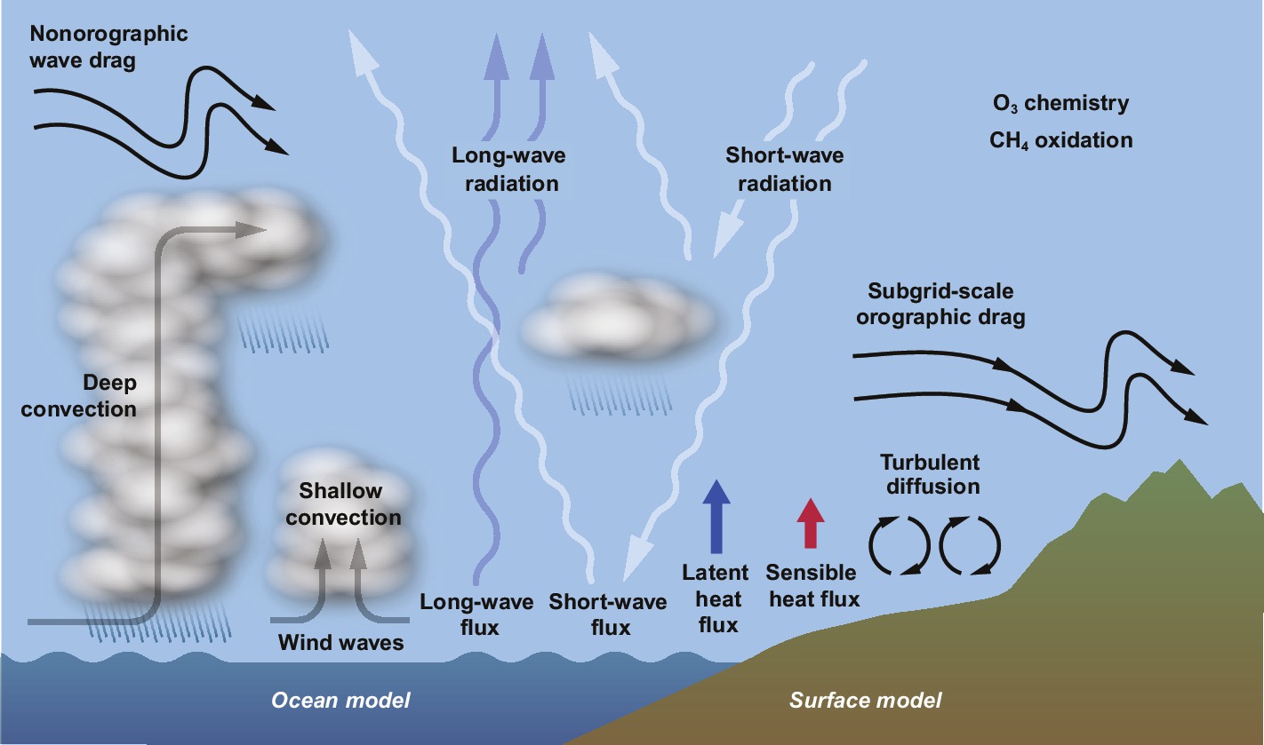
NWP describes the physical and dynamical processes in the atmosphere. It is a method to describe the current and future state of the atmosphere being forced by known physical laws as energy conservation, horizontal and vertical momentum conservation, hydrostatic continuity, and parameterization of subscale phenomena, e.g., cloud-droplet formation (Fig. 8.3). Those partial differential equations are solved on a mesh of grid points. As no analytical solutions are possible, the governing equations have to be solved numerically.
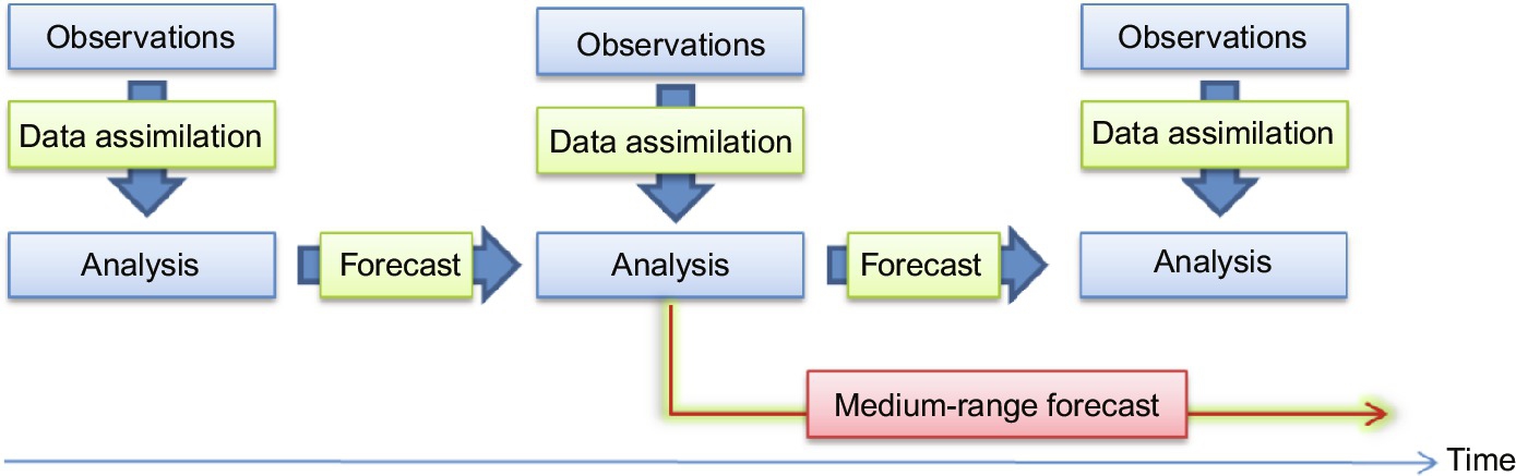
Initial conditions are derived from world-wide weather observations made by ground-based instruments, radiosondes, satellites, etc. They are combined with the analysis (Fig. 8.4), which is the previous NWP forecast state in the so-called data assimilation process. Both error covariance matrices of the observations and the background model state in order to provide an optimum best-of estimate of the atmospheric state. Given that the number of available observations is limited and that parts of the globe are characterized only poorly, the definition of initial conditions is always rather uncertain.
The future state of the atmosphere is calculated by solving numerically the basic partial differential equations forward in time. Processes on scales larger than a grid box are treated explicitly. Atmospheric flow, wind fields, temperature, moisture, and—if available—aerosols are among them. Processes being active on the subgrid scale either in the horizontal or the vertical direction have to be treated by parameterizations. These aim at providing an estimate of the average effect on the main model scale and summarizing the net effect of all small-scale processes inside a grid box. Typically, they deal with a single or a few specific aspects in a physical process only. Any changes in a parameterization may interact in an unforeseen manner with connected physical processes, being treated by another parameterization.
Additionally, some physical processes as turbulence or microphysics of clouds are not fully known on all scales occurring in nature. Other physical processes are highly nonlinear, resulting in difficulties to model them numerically with the required processing speed.
Typically, a global or large-scale model covers the whole Earth. It is used to derive initial conditions as well as boundary conditions for limited area models (LAMs) and to describe the “incoming and outgoing” weather at the LAM border. LAMs provide a finer grid and a higher resolved topography, but they only cover selected regions as e.g. the country of the meteorological service running the LAM and some surrounding area to model upstream weather phenomena. They are also called regional or mesoscale models.
8.2.1.2 Radiative transfer, clouds, and aerosols
Radiative transfer describes the behavior of radiation in the atmosphere. For DNI, the shortwave component directing from the Sun to Earth is the relevant part. The atmosphere is described as a combination of air with several trace gases, clouds, and aerosols by assuming optical properties as refractive indices and scattering phase functions for each part. Modeling radiative transfer is among the most computationally demanding parts of a NWP model. It requires the computation of scattering and absorption processes in a large wavelength domain from the shortwave to the infra-red wavelength range. Please note, that the radiation module in a NWP model does not primarily serve the needs for solar energy users, but is intended to provide the thermodynamic state and especially vertical heating rates in the atmosphere due to incoming and outgoing radiation. Typically the radiation is calculated only every nth time step and on a spatially reduced grid (e.g., Ref. [9]) and is interpolated on the full model grid resolution afterwards.
The circumsolar radiation is treated in several NWP models by the concept of using scaled optical depths (e.g., Joseph and Wiscombe [10], as used in the ECMWF Integrated Forecast System). The strong forward peak of cirrus cloud and aerosol particles is numerically solved by assuming a scattering phase function without forward scattering, but by correcting this assumption by a reduced optical depth. It may create DNI values which are systematically larger than DNI as measured by a pyrheliometer in thin cirrus or aerosol conditions as the effective field of view of this method is larger than the 2.5 degrees half-angle used by the pyrheliometer. Other radiative transfer codes may not treat the forward scattering in the direct irradiance at all (e.g., [11]) and therefore result in a systematic underestimation of the DNI as measured by pyrheliometers. This handling of optical depths has to be checked for each forecast data set in detail.
Talking about irradiance forecasts directly leads to the discussion of the treatment of clouds in NWP. Clouds in the atmosphere are extremely variable in space and time and their optical properties are hardly known. Additionally, their microphysical representation with the help of parameters like cloud droplet radius or effective particle radius or the distribution of liquid and ice water phase with its three-dimensional structure in a cloud is generally not known. On the other hand, all these properties have to be provided in a meaningful average and statistically valid manner on the coarse resolution of the NWP model grid. This requires a number of parameterizations, describing the physical processes in a way so that they are valid at least on average in a grid box.
LAMs are suitable to resolve smaller-scale atmospheric flow phenomena, e.g., land-sea breezes and topographically forced wind flows. Convection schemes typically assume that a grid box is larger than the convective cells and that there are several convective clouds in a grid box. This allows a statistical treatment of an ensemble of convective clouds.
This assumption is not fully valid if the NWP model resolution is only a few km. In high resolution LAMs with a grid box size below ~5 km, the deep convection needs to be explicitly modeled by dynamic and cloud microphysical schemes. Deep convective clouds are typical cloud structures in any precipitating event. Most NWP models treat the deep convection as rising plumes of moist air (so-called mass flux schemes, e.g., Ref. [12]). Common problems include a too early or late triggering of convection, or an inappropriate horizontal evolution of events. Just as an example, we discuss the inhomogeneity effect of clouds: realistic clouds are heterogeneous and therefore show a larger transmission than homogeneous clouds with the same average cloud optical thickness. For example, Tiedtke [13] suggested an inhomogeneity correction factor for COD of 0.7 as input in the radiative transfer scheme. Such kind of parameterizations cannot be applied anymore in a highly resolving model treating deep convection explicitly, as they are only valid on larger spatial scales.
The shallow cumulus convection remains small enough compared to the grid box in large-scale and mesoscale models. NWP models use, e.g., a mass-flux method as for deep convection, but this is valid for an average in the grid box only. Small-scale clouds are closely connected to the modeling of small-scale turbulence being responsible for the vertical heat and moisture transport and therefore for creating water vapor saturation and cloud formation. Various turbulent-transport parameterizations exist, resulting in less or more cloudy boundary layer situations than in reality in many cases. As soon as larger cloud elements are treated explicitly, the mass-flux assumptions do not remain valid for the remaining, unresolved turbulence scales. The treatment of this so-called gray zone of turbulence in the 1–10 km scale is scientifically not finally solved with turbulence modeling knowledge [14].
So, using a LAM does not mean that in shallow convection each cloud can be modeled individually. Such an approach can be made in large eddy simulation models, but they require large computational power. They can be used only for research to study individual clouds and their processes or small ensembles of clouds.
A coupling of micro- and mesoscale modeling is discussed. The micro-scale processes are treated in a large number of slightly varied model runs. Combining these various realizations allows building an ensemble in a grid box which provides the coupling and feedback from the micro- to the mesoscale processes in the model. However, this is very computationally demanding and not available in operational NWP models nowadays.
Subgrid-scale cloud fraction in each vertical layer is modeled in some NWP schemes, while others follow an all-or-nothing strategy assuming that a grid box is either cloudy or not. Cloud fraction may be diagnosed in each model time step or exist as a prognostic variable. A prognostic variable has a time-dependency, follows a conservation law, and can be transported from grid box to grid box like, e.g., moisture. Diagnosed cloud fraction, on the other hand, has no “memory” on previous model states as it is calculated in each time step again, e.g., from liquid-water content.
With respect to radiative transfer calculations, the cloud overlap of convective clouds modeled in various vertical layers needs to be addressed. Clouds in different vertical layers have less impact on irradiances at the ground if they are staggered vertically above each other than if they are distributed randomly in the horizontal [15]. Even if cloud fraction is modeled correctly in each layer, the assumptions on the geometrical position of clouds to each other may cause biases. This effect is smaller in the case of optically thick clouds as the transmission reaches a saturation level. Several parameterizations to define the overlap of cloud layers with different cloud fractions exist. It is discussed that the applied maximum random overlap of clouds is underestimating the column integrated cloud cover and therefore overestimates global horizontal irradiance (GHI) at the surface (e.g., Refs. [16,17]).
Another cloud type with often small horizontal extension of the individual clouds are orographic clouds. They are created by lifting when air is forced to move vertically over rising or inhomogeneous terrain. The air is cooled down adiabatically and condensation starts. Depending on the wind and humidity field structure, these clouds may exist only over mountains and stay at a fixed point. Or an atmospheric gravity wave is forced, resulting in a wave-like cloud structure with a number of repeated small clouds along the direction of movement of the air flow.
Up to now, we have discussed cumulus clouds created by convection processes. Nevertheless, there are also stratiform clouds which cover large geographical areas and are often caused by vertical lifting of large air masses. Additional processes cause fog, but this is of minor relevance in typical CSP regions. Therefore, fog is not discussed further even if it is known that for photovoltaics the restrictions in modeling fog is often critical. Stratiform cloud physical parameters are described by separate microphysical parameterizations. These generally provide the phase (ice or liquid water), the number concentration and the size distribution of hydrometeors such as cloud droplets, rain droplets, and ice crystals. These parameters are vital as input to the radiative transfer module. In particular, a detailed handling of the ice phase is vital for an improved radiative transfer in cirrus and mixed-phase clouds. Depending on the vertical resolution of a NWP model, the correct representation of thin cirrus layers is very difficult, which is critical for the calculation of direct irradiances, and therefore DNI forecasting.
Based on this complexity in the nature of clouds, it is obvious that the correct representation of a single cloud is not feasible in NWP. Therefore, high spatially and temporally resolving NWP models may be capable of resolving cloud processes better, but the individual decision of a cloud existing or not in a grid box average is often wrong. As a result, and with respect to solar irradiances, the so-called double penalty problem of high-resolution NWP models is strongly observed. Generally, it is expected that a higher temporal and spatial resolution of a NWP model results in a more accurate representation of physical processes, and therefore provides more accurate point forecasts. Actually, for irradiances and other local weather parameters this is often not true [18,19] because increasing the model resolution also creates new errors in the spatial location and the timing of individual cloud systems. Let's imagine a cloud system that is in principle correctly predicted, but placed in the wrong grid box. The solution is closer to reality than a large grid box average in a low resolution model, but this is not rewarded. On the contrary, it will be counted once as forecast failure in the box where it appears wrongly and twice as a forecast failure in the box where it should have appeared. So, any location or timing error is counted twice. This effect tends to erase the positive impact of larger spatial and temporal resolution. This often causes better verification scores for lower-resolution models compared to high-resolution NWP models. This occurs especially for the RMSD, as any gross error is emphasized by the square of the error. In meteorological science the traditional verification of geographically matching forecasts and observations may be replaced by a fuzzy verification allowing also neighboring grid boxes to be counted as “success” if a cloud is modeled there when the observation is cloudy. On the other hand the RMSD at a location of interest is the most relevant error measure for many users from the solar electricity grid integration sector and while the neighborhood verification approach is helpful for NWP model developers, it does not reflect the user needs properly.
Besides clouds, the second important parameter is aerosols and their extinction. This is especially valid if DNI is requested. Schroedter-Homscheidt et al. [20] discuss the need for dedicated aerosol forecasts in various regions of the world in a map. Aerosols certainly have to be taken into account close to desert dust sources or in strongly emitting industrial areas. Several NWP schemes apply climatological means (e.g., Ref. [21]) as aerosol representation. Only recently, ECMWF has incorporated an explicit modeling of aerosols within the CAMS in an operational NWP scheme [22,23]. In such an approach, the aerosols should be fully coupled with the meteorology part of the NWP model. Emissions of natural aerosols depend on model surface winds and surface characteristics. Anthropogenic emissions are specified by emission inventories and biomass burning is estimated from space-based fire detection. Such an approach derives both mass concentrations near the surface as also columnar aerosol optical depth (AOD).
Finally, a note about radiative transfer parameterizations. Typically, radiative transfer schemes in NWP models assume a horizontally plane-parallel atmosphere, which is horizontally homogenous. This implies that all three-dimensional effects from any neighboring clouds are neglected when calculating the downwelling irradiance to the surface in the individual grid column. Therefore, overshooting GHI due to three-dimensional effects does not exist in NWP forecasts. Additionally, this implies that cloud cover along the optical path through the atmosphere is not treated explicitly. Only the clouds existing in the grid column above the surface are taken into account in low sun conditions, because the parameterizations is only calculated in the vertical above the gridpoint.
8.2.1.3 Operational considerations on NWP
Operationally available NWP based forecasts can be divided into direct model output (DMO) of a meteorological service NWP model system and statistically adapted, postprocessed products after, e.g., applying a model output statistic (MOS) scheme or any other calibration. Sometimes, the term end products is used for the actual forecast data delivered to the user [24].
A typical LAM area in Europe may cover roughly half or one-third of the European continent. Therefore, any LAM needs initial and boundary conditions from a global model. Most LAMs provide nesting capabilities, allowing a very high spatially resolved “inner nest” in the region of interest which is incorporated in a less resolved model run of the “outer nest” within a single model run. Due to their restricted geographical coverage, LAMs typically do not provide any medium-term forecast, but they often provide a higher temporally resolved DMO of 1 hour or better. On the other hand, LAMs may be started more often than global models in rapid update cycles.
Depending on the scope of the forecast provider, typical refresh rates are between 1 and 6 hours. For global NWP models typical refresh rates are 3 or 6 hours. For regional models, a 3 or 6 hourly restart of the forecast system is used. Rapid update cycling models may start up to every hour. Therefore, several parallel runs of forecasts are valid at the same overlapping time period.
The refresh rate is chosen in relation to the temporal and spatial resolution of the model. Global models have typically coarser spatial resolutions and will miss short-term and small-scale variations in their grid. On the other hand, they run over longer forecast horizons as they focus on modeling the longer-term phenomena in the atmosphere, e.g., the large-scale dynamical flow. Regional models provide finer spatial resolutions and aim at short-term phenomena, e.g., convectional clouds. They are typically started more often, but provide shorter forecast horizons. The meteorological service has to decide for an optimum trade-off between computational times needed for a spatially higher resolved numerical model versus those needed for a longer model horizon.
Please note that the output temporal resolution is much less than the internal model time step, which ranges from seconds to several minutes depending on the numerical stability requirements and the physical process. However, due to storage costs and time limits, the output frequency is typically 1–3 hours, and has only recently been changed to 15 minutes at some meteorological services following the request of electricity markets.
Irradiance parameters are typically given as aggregated integral values since the last model output time step. Section 8.2.3 describes a method to derive higher resolved DNI forecasts with an appropriate temporal interpolation scheme.
GHI are often named shortwave irradiance or downwelling shortwave radiative flux in NWP model output. If available, direct irradiances are also provided and need to be converted to DNI (see Section 8.2.3).
8.2.2 Postprocessing
8.2.2.1 Splitting GHI in DNI if only GHI is forecasted
In many NWP schemes, neither direct horizontal nor direct normal irradiances are part of the prognostic variables in the DMO. Please note that for most NWP models, this is a matter of configuration only. Frequent user requests may change the output structure of the local meteorological service provider. This happened already, e.g., for the IFS at the ECMWF in July 2011 and a few years later at the HARMONIE model system at AEMET or the COSMO model system at Deutscher Wetterdienst.
Nevertheless, the need to convert GHI to DNI remains for many regions in the world and also is needed if any long-term forecast accuracy assessment is done in time periods where the direct irradiances is not provided as DMO.
A number of global-to-diffuse irradiance models exist, which can be also used as global-to-beam models to split GHI into DNI and diffuse components. Frequently used are the DirInt model [25], the Skartveit and Olseth model [26], and the Boland-Ridley-Lauret model [27]. Torres et al. [28] compared a number of global to diffuse conversion models, and Law et al. [29] report about individual validation results from various studies.
8.2.2.2 Converting direct horizontal irradiances into DNI
Generally, direct normal irradiance can be derived from direct horizontal irradiances through a division by the cosine of the sun zenith angle (SZA). The solar zenith angle can, e.g., be computed with the SG2 method [30]. It is recommended to do so in a 1-minute temporal resolution as the SZA is changing quickly.
Often only averaged irradiances or summed irradiation over a time period, e.g., 1 hour, are available and need to be converted into DNI. In this case it is not obvious which SZA shall be taken—the SZA at the beginning, at the end, or the average SZA during the period. And in the case of averaging SZA, should minutes inside the interval before sunrise or after sunset be taken into account or not.
Blanc and Wald [30] evaluated several approaches and recommend the effective solar zenith angle being calculated from an clear-sky model based irradiation in the time interval of interest. A “clear-sky” model describes the irradiation in cloud-free conditions, but taking aerosols, water vapor, and absorbing trace gases into account. This clear-sky model value should be generated by calculating 1-minute irradiation values being summed up or averaged on the time interval being requested. Using, e.g., CAMS McCLear [31] allows to derive the normal and the horizontal direct radiation under cloud-free conditions and by division of these two variables, we can obtain the effective SZA for the time interval of interest.
8.2.2.3 Temporal and spatial interpolation
DMO often provides a 3–6 hourly temporal resolution. Any linear interpolation is not recommended due to the strong diurnal cycle of DNI. Lorenz et al. [32] suggest an interpolation of GHI with the help of a clear-sky model which can also be used for DNI. The clear-sky index kc is defined as the ratio of the actual irradiance value divided by the clear-sky value and the beam clear-sky index is defined as ![]() . The diurnal cycle of irradiance is eliminated by this normalization. The clear-sky index is then interpolated linearly over time and multiplied by the respective clear-sky irradiance to provide the interpolated irradiance value at any point in time (Fig. 8.5).
. The diurnal cycle of irradiance is eliminated by this normalization. The clear-sky index is then interpolated linearly over time and multiplied by the respective clear-sky irradiance to provide the interpolated irradiance value at any point in time (Fig. 8.5).

Generally, in NWP forecast verification the number of grid boxes is larger than the available DNI observations. The closest grid point is usually chosen to perform any verification unless the terrain is very variable or coastlines occur within the grid box. Taking a bi-linear interpolation as being recommended for spatially smooth variables, e.g., temperatures, is not recommended for clouds and irradiances. It should be noted that any verification always has to be treated as a point versus area average verification. Therefore, high scatter and therefore RMSD are to be expected in DNI verification studies. Performing any spatial averaging of DMO DNI values may reduce the RMSD of DNI forecasts by dampening the double penalty problem.
8.2.2.4 Postprocessing based on ground observations
Besides using global-scale NWP as a starting point for a high-resolution regional processing, it is also widely used in postprocessing techniques, e.g., MOS to perform localization. This downscales coarse resolution NWP output to any local features at the location of interest, e.g., due to topography, orography, any local aerosol loads not included in the NWP, e.g., in industrial regions, local cloud features as fog, or higher reflection due to snow.
A MOS approach uses historical forecasts and measurements to derive empirical, site-specific connections between different weather parameters (e.g., Refs. [33,34]). Predictor variables are identified and weighted with regional and seasonal dependencies in order to modify each new forecast value. While large-scale atmospheric features are taken from the input models, the local features are included in a statistical learning process. Applying a MOS requires near-real-time observations to be provided to the meteorological service provider as input. In the commercial sector, GHI forecasting for grid integration of photovoltaic electricity generation often makes use of MOS schemes. Additionally, a MOS will help to provide any bias correction—if needed, in a local area model as well as in a global DMO.
Nevertheless, for DNI forecasts the MOS approach is not widely in use. It is restricted by the need to provide a parameter which is typically driven by small-scale clouds on the subgrid scale while the NWP output is available only with hourly or 3-hourly output frequencies. Only a few meteorological services provide direct irradiances which can be used as predictor. If not available, MOS systems have to derive DNI from predictors as cloud cover and global irradiances only. Knowing additionally that aerosols are not treated in most NWP nowadays, the value of any MOS system in our field is restricted. There is a trend to provide direct irradiances in the NWP DMO and increasing the temporal resolution of the NWP output, and the value of the MOS technique may increase in forthcoming years also in forecasting the DNI.
Other authors apply other machine learning techniques (as discussed in Section 8.3.1) to perform the same tasks of bias correction and localization of DNI. This effort is also sometimes called site adaptation or based on the measure-correlate-predict approach. Typically, and as a rule of thumb, any machine learning is capable of reducing RMSD by 10%–20% at a local point of interest.
8.2.3 NWP-based DNI forecast accuracies
This section provides a short overview on existing NWP-based DNI forecasts and the knowledge about their accuracy. Generally, irradiance evaluations are very much dominated by the selection of stations. Due to the scarcity of good DNI observations, the knowledge cannot easily be transferred to the location of interest. Nevertheless, this section aims at summarizing the existing knowledge.
Generally, there are only a few existing and published studies on DNI forecast accuracy. Therefore, we first summarize the existing knowledge on GHI forecast accuracy. Perez et al. [35] recommend using NWP models if the forecast horizon exceeds 5 hours and to use satellite-based nowcasting for forecast horizons below. Perez et al. [36] compared several global and regional NWP models for the United States, Canada, and Europe. The nRMSE as normalized by mean GHI RMSE ranges between 20% and 69% for US sites, 29% and 44% for Canadian sites, and 40% and 64% in Central European sites for the 1-day ahead hourly resolved forecasts.
Generally, NWP models underestimate clouds and show positive biases of GHI (e.g., Refs. [37,38]). Schroedter-Homscheidt et al. [39] find small negative GHI biases for cloud-free situations and large positive biases for water and mixed phase clouds. For thin ice clouds, biases for some stations are close to zero and for other stations close to or in Northern Africa large positive biases are reported.
Nevertheless, these are numbers for GHI. For DNI generally the error measures show at least twice the values. This is due to the much higher influence of the atmosphere on DNI than on GHI. In particular, thin ice clouds and aerosol loads affect DNI strongly, while for GHI these are small effects. Therefore, any forecast verification results from GHI can only be transferred qualitatively to the DNI forecast in thick cloud conditions.
For DNI, a number of forecast verification studies are described in a review paper by Law et al. [29]. Lara-Fanego et al. [40] showed results for WRF (Weather and Research Forecasting) in Southern Spain for clear-sky conditions with day ahead biases of −6% and 11% at stations Andasol and Cordoba and rRMSD of 22%–24%. These values increase in broken cloud conditions up to 105% and a considerable positive bias between 60% and 72% is observed.
Schroedter-Homscheidt et al. [39] report low biases for cloud-free situations, but large positive biases for thin ice and water/mixed phase clouds for the ECMWF IFS model in hourly resolved day ahead forecasts. Fig. 8.6 (taken from this paper) shows the evolution of rMB and rRMSD over the years 2003–12 in the ECMWF/IFS model at BSRN (Baseline Surface Radiation Network, http://bsrn.awi.de/) stations in Cabauw (NL), Camborne (United Kingdom), Carpentras (F), CENER (E), Izana (E), Lerwick (UK), Lindenberg (D), Palaiseau (F), Payerne (CH), Sede Boker (IL), Tamanrasset (DZ), Toravere (EE), at EnerMENA stations Maan (JO) and Tataouine (DZ), and at the DLR station Plataforma Solar de Almeria (PSA, E). Forecast verification is compared to the 2-day persistence forecast based on ground observations (dotted lines).

Breitkreuz et al. [41] found a reduction of rRMSD for direct irradiances from 31% to 19% for Europe and Northern Africa in clear cases if explicit aerosol modeling was included in a WRF-based scheme.
Having discussed the double penalty problem in cloud and irradiance forecasts, it is not surprising that Lara-Fanego et al. [19] found that higher resolution modeling in WRF did not improve DNI forecast accuracy in cloudy conditions. Also, Mathiesen et al. [37] discuss that spatial averaging reduces the double penalty effect for WRF 2-day ahead DNI forecasts.
8.3 Nowcasting irradiances
8.3.1 Statistical models
For the forecast horizon from minutes up to 1–2 hours, on-site real-time measured DNI and methods like Kalman filtering, moving average, autoregressive moving average, and autoregressive integrated moving average models are used (e.g., Ref. [42]). Based on statistical assessment of a longer time series, relations between predictors (input variables) and predictands (output variables) are defined. Typically, those relations are defined as linear or with a characteristic, deterministic seasonal or daily cycle component plus some random component to describe the variability. Additionally, artificial neural-networks or support vector machines are frequently applied (e.g., Refs. [43–46] comparing GHI forecasts; [47]). They aim at addressing the complex and nonlinear structure of time series.
All statistical methods make use of the high autocorrelation of irradiances for very short time periods due to the solar daily cycle. A word of caution is necessary, as most of these models are used originally for GHI. For GHI, the autocorrelation mostly breaks down in scattered cloud cases only, while DNI is much more sensitive than GHI to the heterogeneous extinction especially in thin cirrus cloud situations. Those are typically very frequent in CSP locations. Therefore, the forecast horizon is very restricted, but the temporal and spatial representativeness can be high if real-time local high quality measurements are available.
8.3.2 All-sky imagers
Tracking the atmospheric flow and therefore the horizontal movement of clouds is the next step to increase the forecast horizon. Such approaches often assume that the cloud shape is kept constant while the cloud is passively advected by the horizontal wind. However, clouds are not passively transported in the air flow. Actually the air flows through the cloudy areas and in areas with suitable humidity and a vertical flow component, clouds are continuously created. Especially in the case of strong thermal processes like, e.g., convection this constant-shape assumption is valid only over short times. Only a few approaches, e.g., Huang et al. [48], start considering cloud deformation.
All sky imagers (ASI) are one technology to monitor horizontal cloud movement. A review of the state of the art is provided by Urquhart et al. [49]. Most ASI systems monitor the sky using a camera with a fish-eye lens looking upwards to the sky. Other designs use a camera that looks downwards on a spherical mirror. Some ASIs use shadowbands in order to avoid reflections of the direct sunlight and partly saturation of the image, but this is a disadvantage because important information on clouds close to the sun is lost. Many ASIs capture red-green-blue images, but some also work with infrared radiation. Current models take images with a resolution of several megapixels, but some older models and infrared cameras with 640×480 pixels are also in use. The bit depth varies from 8 to 16 bit and multiple exposure times may be used by some groups to increase the dynamic range. One image or exposure time series of images is typically collected every 30 seconds or even more often. They are capable to detect short-term ramps due to changes in cloud cover and can resolve cloud and subsequent DNI features in a map within the solar field with a forecast horizon of typically 10 minutes.
In a first step, clouds need to be detected as individual objects. A smoothing is applied to filter very small-scale features which are not predictable in any case. In order to define their position relative to the ground, the cloud height needs to be allocated. Using consecutive images, each cloud object is tracked, e.g., by a maximum cross-correlation technique. Other algorithmic approaches for the pattern matching are summarized in Law et al. [29]. This results in cloud movement vectors which are then applied to the most recent image and provide a prediction of the future cloud mask (Fig. 8.7). The average of several consecutive vectors may be used. Finally, a three-dimensional calculation of DNI at the ground (e.g., Refs. [50,51]) is needed to derive DNI as a function of solar geometry and any assumption on the cloud physical parameters of the individual, already nowcasted cloud and its irradiance extinction coefficient (Fig. 8.8).


This approach has a number of difficulties:
• Clouds are no simple shape objects with clear borders (Fig. 8.9) and therefore, not easy to detect. They may grow, shrink, or turn.

• Most sky cameras lack detailed spectrally resolved observation which would facilitate cloud identification. Cloud index algorithms are frequently used to derive DNI.
• Clouds close to the sun tend to be invisible due to the very bright peak of solar irradiance around the sun disk in the circumsolar area. Depending on the clouds, the area of the circumsolar peak is changing—especially cirrus clouds widen the circumsolar peak and do not allow any a-priori knowledge of the circumsolar peak. On the other hand, these closest to the sun disk positioned clouds are most relevant for the very short-term forecast of the upcoming few minutes.
• Clouds in the outer circle of the fish-eye field of view are located in much larger distance than those close to the camera zenith. Therefore, clouds in the outer circle are seen from the side, while clouds in the zenith are seen from below. Tracking them even if they remain ideally constant in shape and structure is hampered by this effect.
• Cloud base height is generally not known if only one camera is used. Often, clouds in different heights are in the camera field of view at the same time. At least the use of two or more cameras or additional instruments is required. Even rather expensive cloud lidars only measure the cloud height in the zenith above the instrument. Taking any cloud lidar from the nearest airport is valid only in regions with a shallow cumulus cloud situation which has the same cloud base height over large areas of many square kilometers. Such meteorological situations often exist close to oceans and generally in well-mixed boundary layers, but become less likely over the mainland in the case of convective clouds. Satellite-based cloud top heights are much less spatially resolved than the sky camera pixels and can only provide a rough estimate. In addition, the use of multiple ASIs is restricted by the detection of the same cloud if each ASI system is seeing the cloud as an object from a different direction which may be misleading. Another option is to measure the cloud shadow speed and to combine this information with the cloud pixel speed from the camera to derive the cloud base height—but again, this approach is valid for single clouds, yet quickly gets blurred in the case of complex three-dimensional cloud structures. Therefore, the geolocation of the cloud has generally a large error.
Besides all image processing difficulties in sky cameras, the remaining physical restriction for this approach is that low clouds move faster across the field of view than high level clouds. Depending on cloud height, the duration of clouds being visible in the camera's field of view is typically 5–50 minutes.
Overall, the temporal horizon of any cloud tracking based GHI and DNI irradiance forecast is restricted to the interval from a few minutes as lower limit up to an upper limit between 10 and 20 minutes (e.g., Refs. [52,53]). Known DNI accuracies from ground-based cloud motion vector tracking are discussed in Law et al. [29]. It should be noted that these studies typically use a restricted number of days only and are hardly comparable as covering different regions. They may serve as a first overview, but may not be generalized.
8.3.3 Satellites
For the forecast horizon between 1 and 6 hours, the movement of clouds is the dominating parameter, while the temporal correlation length of aerosols is typically longer. Schepanski et al. [54] have shown this explicitly for the dust aerosol component.
The movement of clouds can be tracked in satellite imagery from geostationary satellites. Meteosat Second Generation (MSG) with its Spinning Enhanced Visible and Infrared Imager (SEVIRI) instrument provides observations in 12 spectral channels in a 15-minute interval over Europe, Africa, the Middle East, and parts of Brasilia. Depending on the location and the spectral channel used, the spatial resolution is between 1 and 5 km. This allows the retrieval of cloud physical properties instead of using semiempirical cloud index methods. Similar capabilities exist in Asia with the Himawari satellite and are expected for the Americas with the GOES-R satellite series to be launched.
Satellite-based cloud motion tracking is a long-existing technology and has been used in meteorology for a long time (e.g., Schmetz et al. [55]; or the review provided by Menzel [56]). For the solar sector and based on cloud index methods, Hammer et al. [57] and Taniguchi et al. [58] applied a similar strategy.
Their principles are the same as discussed for sky cameras (Fig. 8.7), with some satellite specifics:
• For MSG or similar instrumentation, cloud detection can be performed more accurately on the basis of more spectral channels in the visible and the infrared range, but with less spatial and temporal resolution.
• Secondly, cloud physical properties as optical depth or effective particle radius are available as additional information. This allows a full physical treatment of radiative transfer as well as the cloud-index approach (e.g., Ref. [59]) used for the broadband satellite instruments, e.g., of the Meteosat First Generation.
• Cloud height is of less importance, as the satellite aperture angle is much larger, and therefore the projection to a parallel plane to the Earth surface is less sensitive to the cloud height. Additionally, thin ice clouds as cirrus in higher altitudes can be separated from low-level clouds spectrally and tracked separately.
• Cloud motion cannot be tracked by a single cloud movement vector per image anymore, but has to be done on a regular grid or on the basis of each cloud system separately. This particularly contributes to the restrictions of this approach, as any change in the shape of clouds is neglected in the cloud motion vector method.
Such approaches are restricted by the fast evolution of cloud systems. Besides lateral movements, cloud systems turn, grow, shrink, change their structure, and even disappear between consecutive images. Additionally, the definition of the exact outer border of a cloud cannot be easily made—neither in high resolution if looking at a cloud with its fluffy edges, nor in a satellite image with a pixel size of typically several square kilometers. Therefore, accuracy of cloud tracking is restricted compared to the tracking of any fixed objects, e.g., in image processing in industrial automatization. But in principle the same optical flow algorithms can be applied as discussed in, e.g., Lucas and Kanade [60].
Once the cloud field is forecasted, any cloud-to-irradiance algorithm can be used as discussed in Chapter 2. Frequently used methods derive the cloud index first and generate a cloud index nowcast as a second step, before a cloud index to irradiance algorithm is applied (e.g., Refs. [59,61,62]). Alternatively, one can use a physical cloud property retrieval scheme (e.g., Ref. [63]) and afterwards a fast parameterization of radiative transfer modeling (e.g., Ref. [64]). As for most NWP-based studies, existing satellite-based studies also typically evaluate GHI nowcasting. Perez et al. [35] showed that cloud motion vector-based GHI nowcasting performs better than NWP up to 4–6 hours.
8.4 Future developments
8.4.1 Rapid update NWP
Within rapid-update model cycles (RUC), the initialization of the NWP model is performed more often, e.g., hourly or 3-hourly compared to a 3- or 6-hourly standard mode. This allows the incorporation of more recent observations and provides more frequent updates of the forecast to the users. However, on the other hand, it also requests observations to be available within shorter assimilation windows. The time being allowed for any observation to reach the meteorological center is smaller and the observations need to be provided more frequently. It is a trade-off being performed by the meteorological services. RUC is being implemented at several NWP centers and was found to reduce the standard deviation of forecast errors for global irradiances. The value of this approach for DNI forecasting is under evaluation currently, e.g., at the Spanish AEMET center.
8.4.2 Assimilating cloud information
Having discussed the difficulties in modeling clouds in NWP, the use of cloud observations in a data assimilation scheme is a more recently investigated option. It is hoped that introducing additional observations increases the model information content in the actual meteorological situation. This may fill the gap in knowledge and capacity to resolve cloud processes properly in NWP. However, assimilating cloud observations requires knowledge to describe the impact of clouds on the model state and vice versa. Suitable parameterizations and simplifications describing the role of clouds are needed in the data assimilation procedure. Several meteorological centers worked on the assimilation of cloud properties (e.g., Refs. [65,66]) and evaluated the impact on low clouds and fog, and on surface irradiances.
Mathiesen et al. [37] assimilated cloud cover in a direct cloud assimilating version of WRF by altering the water vapor mixing ratio and investigated the GHI forecast accuracy. The scheme was successful in cloudy situations, but failed in clear-sky conditions, as cloud dissipation was not modeled accurately.
Typically, a positive impact in the nowcasting range up to 3 or 6 hours is found with the currently used assimilation schemes (e.g., Refs. [66,67]). A longer positive impact would require not only changing humidity and cloud fields in the model, but also changing dynamics and thermodynamics consistently, which complicates the approach. These results support using such approaches preferably in rapid update cycling NWP models.
8.4.3 Including explicit modeling of aerosols
Breitkreuz et al. [41] used explicitly modeled AOD values and showed improvements over climatological aerosol databases in the cloud-free case. Ruiz-Arias et al. [68] showed that using the WRF model with additional aerosol input increased clear-sky DNI forecast accuracy. Coupling air quality modeling with NWP and aerosol observations is therefore recommended for a good DNI forecast in cloud-free conditions.
In particular, for the CSP sector this is critical as cloud-free situations are dominant in typical CSP locations. Nevertheless, the typical mass mixing ratio modeling approach in the air quality field needs to be extended to columnar AOD as model output to make is usable in DNI calculations. Schroedter-Homscheidt et al. [69] investigated the need for daily updated aerosol information by using ground-based aerosol observations both as ground truth and as ideal forecast. Recently, aerosol forecasts have been introduced in the ECMWF's NWP model by the CAMS. It was shown that these new forecasts are more accurate or equal to a 2-day persistence method in Europa and America, but not in eastern Asia and western Africa.
8.4.4 Soiling
Soiling of plant components has a large effect on the plant efficiency as discussed already in previous chapters. After developing a method for real-time measurement of the mirror cleanliness [70], researchers are now investigating options to model the soiling rate based on meteorological variables that are available from simple measurements, NWPs, or chemical transport models. Such models might also provide forecasts of the soiling rate in the future. Extreme soiling events connected to sand and dust storms can already be predicted (e.g., WMO's SDSWAS [71]), although no quantitative prediction of the reduction of the cleanliness is possible so far.