
Pivot magic
This chapter draws together the technical discussion in the previous chapters to arrive at the point where readers will be able to create robust user-friendly spreadsheets that they will be proud of distributing. More importantly readers that follow these instructions will be able to very quickly and accurately interrogate their operational data. This chapter explains step-by-step how to create pivot tables, and explains how to create a template that can be used to manage all your spreadsheets. On completion of this chapter, readers will be able to produce robust spreadsheets that have a consistent look and feel, and from a user’s point of view, look more like a word document than a spreadsheet.
Keywords
Pivot tables; user friendly spreadsheets; spreadsheet distribution; data interrogation; operational data analysis; spreadsheet template
This is the chapter where the threads of everything discussed so far finally start to come together. When I was thinking about the structure of the book I faced a dilemma. On one hand the importance of things such as raw data structure and data validation only make sense when you understand how pivots work. On the other hand, you cannot build functioning pivots unless you know how to structure your raw data properly, and you use data validation. My approach, in the end, was to start from the foundations, and work my way up, and in doing so hoping that the readers would stick with it, understanding that it would be worth it in the end. Once you have started using pivots properly, you will wonder how you ever managed without them.
So, after having made such a fuss about pivots, what is the big deal? Pivots allow you to slice and dice data VERY quickly. They also allow you to present that data in a multitude of ways, and do that very quickly too.
How to create a pivot table
There are only a few steps involved in creating a pivot table:
1. Go to the insert pivot table menu. In Excel 2010, you click on the “Insert” menu, then select the “PivotTable” icon on the far left. This will result in the following dialogue box opening:

2. Define the Table/Range the pivot table should cover. You can do this by selecting a range, or using a dynamic named range. Selecting a range is a bad idea. As you add data you want the pivot table to automatically grow to capture this new data. If you select a range, then it will stay fixed to that range, even if you add new data. You can manually extend the range, but firstly it is very easy to forget doing this, and secondly, if you have a lot of pivots, in a lot of spreadsheets, then it will become too time consuming. Hard wiring in the range is lazy and costly. The best option is to use a dynamic named range. This is discussed in the previous chapter, but in case you forgot here is an example of the formula, with each of the bolded parts explained in turn, where the dynamic named range refers to the below raw data for visits:

• =OFFSET(RawData!$B$10,0,0,COUNTA(RawData!$B$10:$B$60000),11). RawData! is the name of the worksheet on which your pivot table is based. As a matter of good practice, all your raw data should be stored in the one range, and all raw data sheets should be called the same name. A sensible name, therefore, is RawData!
• =OFFSET(RawData!$B$10,0,0,COUNTA(RawData!$B$10:$B$60000),11). $B$10 is the top left hand cell in your raw data range. In other words, it is your first header, which in this example is “Date.”
• =OFFSET(RawData!$B$10,0,0,COUNTA(RawData!$B$10:$B$60000),11). $B$10:$B$60000 is the range of data that the formula will perform a COUNTA on. This formula counts the number of non-blank cells in the range between cells B10 and B60000. The number of non-blank cells counted by the formula will determine how many rows will be captured by the pivot table. For this formula to work there cannot be any blank cells in column B. As a rule there should not be any blank cells anyway, but if there is even a small risk that someone will enter a row of data, and leave column B blank, then you will need to do a count on a different column. Also, if you are expecting to enter more than 60,000 rows of data, you will need to change the 60,000 part of the formula to a larger number.
• =OFFSET(RawData!$B$10,0,0,COUNTA(RawData!$B$10:$B$60000),11). 11 is the number of columns of data you want the pivot table to cover. You could make this dynamic too, but it’s honestly not worth the effort. Just remember, if you have 11 columns of data, and you add a new column, and you want that column to be captured by the pivot table, you will have to change the “11” in this formula to “12.”
All of the above might sound like a lot of work, maybe you think its too much effort. Take my word for it, after you have used this formula once, it will be easy to amend when you create a new pivot table. If you keep your raw data structure consistent, and you should, then the only thing you will most likely need to change after you have used the formula once, is the number of columns (i.e., the number 11 at the end of the above formula). Once you have used a dynamic named range, you have set and can forget your pivot data source.
3. The last step is to choose where you want the pivot table to be placed. This should not be on the raw data sheet. The raw data sheet should be reserved entirely for data entry, for reasons that have already been discussed. The section called “Bringing it altogether” discusses where to place the pivots for maximum impact. For the moment, given you are only practicing, it does not matter where you place the pivot.
Anatomy of a pivot table
After you click OK on the Create PivotTable dialogue box, Excel will create a blank pivot table that will look something like the following:

Don’t worry about the appearance of the term “fields,” they are just your headers. You can drag any of these fields to one of four boxes, Report Filter, Column Labels, Row Labels, and Values. Each of these boxes has a unique function.
• Values – this is what you will be counting, it is the measure. For example, if you wanted to know the size of your collection you could do it several ways. You might count the number of unique titles or you might count the number of items. The values section of the pivot table determines what you are counting, and how you are counting it (e.g., as a count, sum, average, minimum, maximum).
• Column and row labels – this is how you are aggregating your data. For example you might want to know the number of library visits by Month and by library Location. If so, you would drag Month into the Column Labels box, and Location into the Row Labels Box, or vice versa.
• Report filter – this is used to limit the information displayed in the pivot to a subset of data. For example, if you wanted to see library visits by Month and Location, you are probably only going to want to see the data for a specific year. If you drag the Year field into the “Report Filter” box, then you will have the option of filtering down to a specific year.
The pivot table will automatically update as you drag fields into the Report Filter, Column Labels, Row Labels, and Values boxes. The thing you will not see as you build the pivot, is the “Slicer”, the box that contains days of the week. Slicers work just like the report filter, except that they are easier to read and change. If you only wanted to see data for visits on Mondays, then you could just click on Monday on the slicer. If you wanted to see data for just Mondays and Thursdays, then you would hold down the control key (Ctrl), and click on Thursday. So slicers allow you to filter data quickly, and you can see what the data is filtered to at a glance. The only cost is that they take up a lot more real estate on your spreadsheet.

Slicers may not be available in all versions of Excel. To add slicers in Excel 2010 you will need to click on the pivot table to activate the “PivotTable Tools” menu, then under “Options” select the Insert Slicer icon.
You can also filter on multiple items in a Report Filter. For example, click on the inverted triangle next to the Year filter on the pivot table, check the multiple items box, and then select the years you wish to include in the report. You can also use these controls on the Row and Columns fields to filter out items, and to sort the lists.
Bringing it all together
The objective off all of the processes I have encouraged you to follow so far is to create spreadsheets that are robust and easy to use. By robust, I mean that you can depend upon the data. The data will be accurate, up-to-date, and complete. The spreadsheets will be robust for the following reasons:
• They will be easy to use, and therefore they will be used more often, and more likely to be used correctly. They will be easy to use because all your spreadsheets will have a consistent look and feel. If a user is familiar with one sheet, it will not be a big learning curve for them to become familiar with another. I am yet to encounter a type of data that can be managed in a standard spreadsheet that could not be managed using a standardized format. Your spreadsheets will also be easy to use because you will only show users the information they need to see. All the formulas they don’t need to see will be hidden. All the sheets they don’t need to see will be hidden. Users should only really ever need to see four sheets at most: “RawData” sheet, “Contents” sheet, “Pivot” sheet, and in some cases the “Validation” sheet.
• You will have policies in place supported by lockdown periods to ensure that data is updated by specific dates, such as every quarter.
• You will have strong data validation rules in place to ensure that users can only enter allowable data types.
• You will take the headache out of reporting, giving managers an incentive to support your standardization drive.
• You will make data more accessible, enabling, at the very least, the possibility of turning data into actionable intelligence. If you can achieve this, then you will provide the executive and the managers’ further incentive to support standardization.
There are a few last things you need to do before you can say you have created a robust spreadsheet, including setting up the Contents, Pivot, Validation, and RawData sheets.
Set up the Contents sheet
The Contents sheet will allow users to quickly navigate to any “precanned” view you have created. The best way to do this is to create a table number that is completely unique; for example, by combining the acronynm for the spreadsheet with a sequential number. That way when anyone talks about table LV1, you will know that they are refering to Table1 in the Library Visits spreadsheet.
To turn the table number into a hyperlink, right click over the table number cell (e.g., LV1), then click “Hyperlink.” There are several things you can link to. Click on “Place in this Document,” then click on the “Pivot” sheet, and then add a cell reference. For the first sheet I am linking to cells A1:A51. I will hide column A in the “Pivot” sheet, so as that the user will not see the cells being selected. The purpose of using the range A1:A51 is to ensure that no matter which cell the user had previously activated in the “Pivot” sheet, the user will always be centered on the relevant pivot table when they click on any hyperlink in the “Contents” sheet.

I place all the Pivots on the same sheet, to reduce complexity. However, to do this successfully, you have to make sure that no matter how many rows the Pivot Table occupies, that it will not overwrite another Pivot Table. One Pivot Table cannot overwrite another, so if you have them overlapping, or a refresh causes them to overlap, then an error will occur, and the pivots will not refresh. The simple solution is to take advantage of the large number of rows at your disposal. So I separate all my pivots by a 1000 rows. This means the link for LV2 will be A1000:A1051, and for table LV3, it will be A2000:A2051. It is highly unlikely that you will create a spreadsheet where a user needs 1000 rows in a Pivot Table, so this is a safe approach.
Obviously, you will need to add a table description, and hide things that the user does not need to see in the “Contents” sheet, such as the headers, and the gridlines (via the View menu in Excel 2010). When you have done this you will end up with a nice clean “Contents” page that looks more like a Word document, and should be reasonably self explainatory to all users.
Obviously you can have more tables if you want, and you can always present them in groups of related tables, by, for example, placing related tables underneth each other, and applying the same color shading to those set of tables. Whatever you do, just make it consistent for all your spreadsheets.
Set up the Pivot sheet
Once you have created the “Contents” sheet, and you are sure you have the views you expect most users will want to see, then you can start creating the Pivots for each link on your Contents sheet. First, hide column A in the Pivots sheet. I added the title for the LV1 pivot to cell C2. The purpose of this is so as that when I turn off the headers and gridlines, there is a bit of white space above and to the left of the table heading (i.e., row 1 and column B is the white space). This makes it a lot easier for users to read your pivots.

You will also notice that I use a formula to define the pivot title in the above screenshot. That way, if I change a table title on the Contents sheet, it will be automatically updated on the Pivot sheet.
The next step is to insert a pivot table. Remember that you are using a dynamic named range as the Pivot Table data source. Add the pivot at least ten rows down from the title, that way you will have plenty of space to insert your report filters. After you are certain you have included all the report filters you are likely to need, then drag the Pivot Table so as that it starts two rows below the heading, or whatever gap you want, so long as it is consistent.
After you have dragged the relevant fields into the relevant parts of the Pivot Table, you will notice that all the column widths readjust. Personally, I don’t like this behavior, and it is problematic when you have all your Pivots starting in the same column. So I prefer to switch this behavior off, by right clicking the Pivot Table, and selecting “PivotTable Options,” clicking on the layout and format tab, then deselecting “Autofit column widths on update.”
You might also wish to add a chart next to your pivot. To create a PivotChart, click on the Pivot Table to activate it, click on insert, then select a chart. This way, each time a user clicks on a link in your contents page, they will be taken through to a clean and easy to read screen.
Another option I highly recommend you change while you have the PivotTable Options dialogue box open is to show blanks for error values, and on the “Data” tab disable “Enable show details,” and enable “Refresh data when opening the file.” The latter is self explainatory. You might find it useful to use the “Enable show details” function, but it will only cause confusion for users if they accidently create a drill through report.
Once you have all your pivot table options set, and you are definitely happy with them, I highly recommend that you simply copy the pivot table, then paste it wherever you need another pivot. This will save you having to set the options for each and every pivot.
To insert the other two pivots just follow the same procedure. For example, the heading for LV2 would be entered into cell B1001 (using a formula!), etc. When a user clicks on a link in your contents page it should take them to the relevant pivot.
Set up the RawData sheet
Your RawData sheet should look something like that shown here, with all the information that the users do not need to see hidden:

If you use borders for all the rows that have a formula, then it will be obvious when data is being entered in rows without formulas. Once again, the aim is to have a clean and consistent format. You need to have data validation on every single visible column, i.e., data validation for Date, Time, SensorID, and Number. This dramatically reduces the risk that users will enter incorrect data.
These sheets can be a bit tricky for data entry when there is more than one person entering the data. In practice it will be difficult for users to find the last row of data they entered, without scrolling through a long list, and perhaps getting it wrong. The solution to this is to include this data in the spreadsheet.

This why it is handy to not have your raw data header start until row 10, as you can squeeze in this sort of information where necessary. If you always keep your header in the same row, that means you can use a script later on to automate much of the work involved in your spreadsheets. It also means you can set up a template.
The formula in the above screenshot has to be entered as an array to work. The way to enter an array formula is to type in the formula, e.g., =MAX(IF(D:D=D6,B:B,“”)), then press Ctrl and Shift and Enter. This last action will convert the formula into an array formula. You can’t do this simply by typing in the {} characters.
Set up the Validation sheet
In most instances you should be able to hide the Validation sheet from users. However, on the chance that you will need users to be able to change validation lists, then you should set these up consistently too. Here is a screenshot of the Validation sheet for the Library Visits sheet.
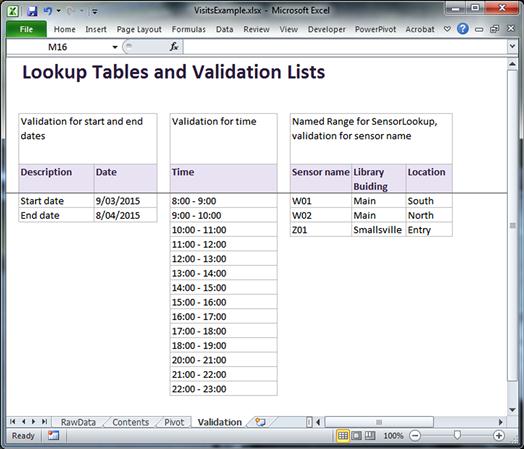
Notice the clean layout, and that information is included above each validation or lookup reference to explain what function the data below it perform. Even if your users do not see this sheet, you should still keep it consistent to make your life easier. If your users do need to update the validation lists, then in might be easier to use tables (see earlier discussion).
Done!
So now you should have a very simple spreadsheet, with only three to four visible sheets. Data entry staff will always know that they can enter data by going to the RawData sheet. Managers will always know they can access their reports via the Contents sheet. And the spreadsheet administrator will always be able to adjust the data validation by accessing the Validation sheet.
If you had your thinking cap on while reading this, you might have realized that you can create a template, save it somewhere safe, and then use that to create any future spreadsheets. Doing this will also ensure that the worksheets are consistent. So do it!