Switching
In the early years of telephones, the telephone operator helped knit together the social fabric of a community. If John wanted to talk to Martha, John would call the operator and ask for Martha; the operator would then manually plug a wire into a patch panel that connected John’s telephone to Martha’s. The switchboard, of course, allowed parallel connections between disjoint pairs. James could talk to Mary at the same time that John and Martha conversed. However, each new call could be delayed for a small period while the operator finished putting through the previous call.
When transistors were invented at Bell Labs, the fact that each transistor was basically a voltage-controlled switch was immediately exploited to manufacture all-electronic telephone switches using an array of transistors. The telephone operator was then relegated to functions that required human intervention, such as making collect calls. The use of electronics greatly increased the speed and reliability of telephone switches.
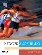
A router is basically an automated post office for packets. Recall that we are using the word router in a generic sense to refer to a general interconnection device, such as a gateway or a SAN switch. Returning to the familiar model of a router in Figure 13.1, recall that in essence a router is a box that switches packets from input links to output links. The lookup process (B1 in Figure 13.1), which determines which output link a packet will be switched to, was described in Chapter 11. The packet scheduling done at the outbound link (B3 in Figure 13.1) is described in Chapter 14. However, the guts of a router remain its internal switching system (B2 in Figure 13.1), which is discussed in this chapter.
This chapter is organized as follows. Section 13.1 compares router switches to telephone switches. Section 13.2 details the simplicity and limitations of a shared memory switch. Section 13.3 describes router evolution, from shared buses to crossbars. Section 13.4 presents a simple matching algorithm for a crossbar scheduler that was used in DEC’s first Gigaswitch product. Section 13.5 describes a fundamental problem with DEC’s first Gigaswitch and other input-queued switches, called head-of-line (HOL) blocking, which occurs when packets waiting for a busy output delay packets waiting for idle outputs. Section 13.6 covers the knockout switch, which avoids HOL blocking, at the cost of some complexity, by queuing packets at the output.
Section 13.7 presents a randomized matching scheme called PIM, which avoids HOL blocking while retaining the simplicity of input queuing; this scheme was deployed in DEC’s second Gigaswitch product. Section 13.8 describes iSLIP, a scheme that appears to emulate PIM, but without the use of randomization. iSLIP is found in a number of router products, including the Cisco GSR. Since iSLIP works well only for small switches of at most 64 ports, Section 13.9 moves on to cover the use of more scalable switch fabrics. It first describes the Clos fabric, used by Juniper Networks T-series routers to build a 256-port router.
Section 13.9 also introduces the Benes fabric, which can scale to even larger numbers of ports and handles multicast well. A Benes fabric is used in the Washington University WUGS switch. Section 13.10 shows how to scale switches to faster link speeds by using bit-slice parallelism and by using shorter fabric links as implemented in the Avici TSR.
The literature on switching is vast, and this chapter can hardly claim to be representative. I have chosen to focus on switch designs that have been built, analyzed in the literature, and actually used in the networking industry. While these choices clearly reflect the biases and experience of the author, I believe the switches described in this chapter (DEC’s Gigaswitch, Cisco’s GSR, Juniper’s T-series, and Avici’s TSR) provide a good first introduction to both the practical and the theoretical issues involved in switch fabrics for high-speed routers. A good review of other, older work in switching can be found in Ahmadi and Denzel [AD89], A more modem review of architectural choices can be found in Turner and Yamanaka [TY98],
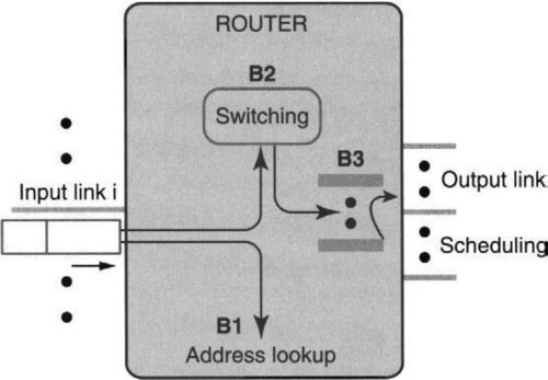
The switching techniques described in this chapter (and the corresponding principles invoked) are summarized in Figure 13.2.
13.1 ROUTER VERSUS TELEPHONE SWITCHES
Given our initial analogy to telephone switches, it is worthwhile outlining the major similarities and differences between telephone and router switches. Early routers used a simple bus to connect input and output links. A bus (Chapter 2) is a wire that allows only one input to send to one output at a time. Today, however, almost every core router uses an internal crossbar that allows disjoint link pairs to communicate in parallel, to increase effective throughput. Once again, the electronics plays the role of the operator, activating transistor switches that connect input links to output links.
In telephony, a phone connection typically lasts for seconds if not for minutes. However, in Internet switches each connection lasts for the duration of a single packet. This is 8 nsec for a 40-byte packet at 40 Gbps. Recall that caches cannot be relied upon to finesse lookups because of the rarity of large trains of packets to the same destination. Similarly, it is unlikely that two consecutive packets at a switch input port are destined to the same output port. This makes it hard to amortize the switching overhead over multiple packets.
Thus to operate at wire speed, the switching system must decide which input and output links should be matched in a minimum packet arrival time. This makes the control portion of an Internet switch (which sets up connections) much harder to build than a telephone switch. A second important difference between telephone switches and packet switches is the need for packet switches to support multicast connections. Multicast complicates the scheduling problem even further because some inputs require sending to multiple outputs.
To simplify the problem, most routers internally segment variable-size packets into fixed-size cells before sending to the switch fabric. Mathematically, the switching component of a router reduces to solving a bipartite matching problem: The router must match as many input links as possible (to as many output links as possible) in a fixed cell arrival time. While optimal algorithms for bipartite matching are well known to run in milliseconds, solving the same problem every 8 nsec at 40 Gbps requires some systems thinking. For example, the solutions described in this chapter will trade accuracy for time (P3b), use hardware parallelism (P5) and randomization (P3a), and exploit the fact that typical switches have 32–64 ports to build fast priority queue operations using bitmaps (P14).
13.2 SHARED-MEMORY SWITCHES
Before describing bus- and crossbar-based switches, it is helpful to consider one of the simplest switch implementations, based on shared memory. Packets are read into a memory from the input links and read out of memory to the appropriate output links. Such designs have been used as part of time slot interchange switches in telephony for years. They also work well for networking for small switches.
The main problem is memory bandwidth. If the chip takes in eight input links and has eight output links, the chip must read and write each packet or cell once. Thus the memory has to run at 16 times the speed of each link. Up to a point, this can be solved by using a wide memory access width. The idea is that the bits come in serially on an input link and are accumulated into an input shift register. When a whole cell has been accumulated, the cell can be loaded into the cell-wide memory. Later they can be read out into the output shift register of the corresponding link and be shifted out onto the output link.
The Datapath switch design [Kan99, Kes97] uses a central memory of 4K cells, which clearly does not provide adequate buffering. However, this memory can easily be implemented on-chip and augmented using flow control and off-chip packet buffers. Unfortunately, shared-memory designs such as this do not scale beyond cell-wide memories because minimum-size packets can be at most one cell in size. A switch that gets several minimum-size packets to different destinations can pack several such packets in a single word, but it cannot rely on reading them out at the same time.
Despite this, shared-memory switches can be quite simple for small numbers of ports. A great advantage of shared-memory switches is that they can be memory and power optimal because data is moved in and out of memory only once. Fabric- or crossbar-based switches, which are described in the remainder of this chapter, almost invariably require buffering packets twice, potentially doubling memory costs and power costs. It may even be possible to extend the shared-memory idea to larger switches via the randomized DRAM interleaving ideas described in Section 13.10.3.
13.3 ROUTER HISTORY: FROM BUSES TO CROSSBARS
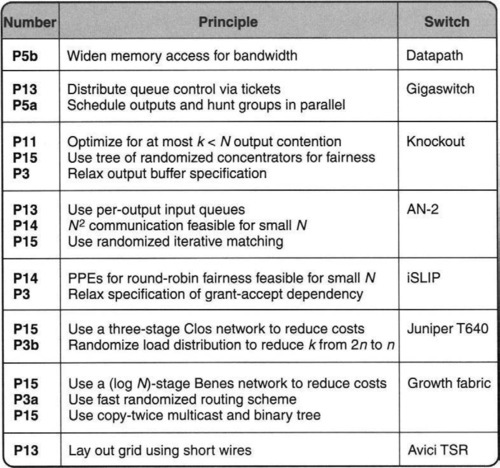
Router switches have evolved from the simplest shared-medium (bus or memory) switches, shown in part A of Figure 13.3, to the more modern crossbar switches, shown in part D of Figure 13.3. A line card in a router or switch contains the interface logic for a data link, such as a fiber-optic line or an Ethernet. The earliest switches connected all the line cards internally via a high-speed bus (analogous to an internal local area network) on which only one pair of line cards can communicate at a time. Thus if Line Card 1 is sending a packet to Line Card 2, no other pair of line cards can communicate.
Worse, in more ancient routers and switches, the forwarding decision was relegated to a shared, general-purpose CPU. General-purpose CPUs allow for simpler and easily changeable forwarding software. However, general-purpose CPUs were often slow because of extra levels of interpretation of general-purpose instructions. They also lacked the ability to control realtime constraints on packet processing because of nondeterminism due to mechanisms such as caches. Note also that each packet traverses the bus twice, once to go to the CPU and once to go from the CPU to the destination. This is because the CPU is on a separate card reachable only via the bus.
Because the CPU was a bottleneck, a natural extension was the addition of a group of shared CPUs for forwarding, any of which can forward a packet. For example, one CPU can forward packets from Line Cards 1 through 3, the second from Line Cards 4 through 6, and so on. This increases the overall throughput or reduces the performance requirement on each individual CPU, potentially leading to a lower-cost design. However, without care it can lead to packet misordering, which is undesirable.
Despite this, the bus remains a bottleneck. A single shared bus has speed limitations because of the number of different sources and destinations that a single shared bus has to handle. These sources and destinations add extra electrical loading that slows down signal rise times and ultimately the speed of sending bits on the bus. Other electrical effects include that of multiple connectors (from each line card) and reflections on the line [McK97].
The classical way to get around this bottleneck is to use a crossbar switch, as shown in Figure 13.3, part d. A crossbar switch essentially has a set of 2N parallel buses, one bus per source line card and one bus per destination line card. If one thinks of the source buses as being horizontal and the destination buses as being vertical, the matrix of buses forms what is called a crossbar.
Potentially, this provides an N-fold speedup over a single bus, because in the best case all N buses will be used in parallel at the same time to transfer data, instead of a single bus. Of course, to get this speedup requires finding N disjoint source–destination pairs at each time slot. Trying to get close to this bound is the major scheduling problem studied in this chapter.
Although they do not necessarily go together, another design change that accompanied crossbar switches designed between 1995 and 2002 is the use of special-purpose integrated circuits (ASICs) as forwarding engines instead of general-purpose CPUs. These forwarding engines are typically faster (because they are designed specifically to process Internet packets) and cheaper than general-purpose CPUs. Two disadvantages of such forwarding engines include design costs for each such ASIC and the lack of programmability (which makes changes in the field difficult or impossible). These problems have again led to proposals for faster but yet programmable network processors (see Chapter 2).
13.4 THE TAKE-A-TICKET CROSSBAR SCHEDULER
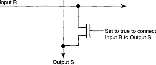
The simplest crossbar is an array of N input buses and N output buses, as shown in Figure 13.4. Thus if line card R wishes to send data to line card S, input bus R must be connected to output bus S. The simplest way to make this connection is via a “pass” transistor, as shown in Figure 13.5. For every pair of input and output buses, such as R and S, there is a transistor that when turned on connects the two buses. Such a connection is known as a crosspoint. Notice that a crossbar with N inputs and N outputs has N2 crosspoints, each of which needs a control line from the scheduler to turn it on or off.
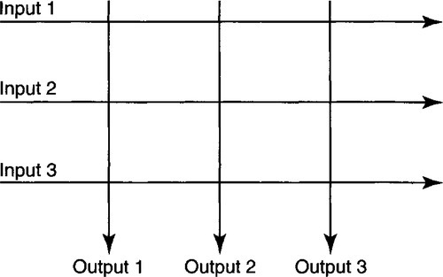
While N2 crosspoints seems large, easy VLSI implementation via transistors makes pin counts, card connector technologies, etc., more limiting factors in building large switches. Thus most routers and switches built before 2002 use simple crossbar-switch backplanes to support 16–32 ports. Notice that multicast is trivially achieved by connecting input bus R to all the output buses that wish to receive from R. However, scheduling multicast is tricky.
In practice, only older crossbar designs use pass transistors. This is because the overall capacitance (Chapter 2) grows very large as the number of ports increases. This in turn increases the delay to send a signal, which becomes an issue at higher speeds. Modem implementations often use large multiplexer trees per output or tristate buffers [All02, Tur02]. Higher-performance systems even pipeline the data flowing through the crossbar using some memory (i.e., a gate) at the crosspoints.
Thus the design of a modern crossbar switch is actually quite tricky and requires careful attention to physical layer considerations. However, crossbar-design issues will be ignored in this chapter in order to concentrate on the algorithmic issues related to switch scheduling. But what should scheduling guarantee?
For correctness, the control logic must ensure that every output bus is connected to at most one input bus (to prevent inputs from mixing). However, for performance, the logic must also maximize the number of line-card pairs that communicate in parallel. While the ideal parallelism is achieved if all N output buses are busy at the same time, in practice parallelism is limited by two factors. First, there may be no data for certain output line cards. Second, two or more input line cards may wish to send data to the same output line card. Since only one input can win at a time, this limits data throughput if the other “losing” input cannot send data.
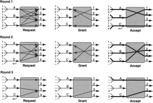
Thus despite extensive parallelism, the major contention occurs at the output port. How can contention for output ports be resolved while maximizing parallelism? A simple and elegant scheduling scheme for this purpose was first invented and used in DEC’s Gigaswitch. An example of the operation of the so-called “take-a-ticket” algorithm [SKO+94] used there is given in Figure 13.6.
The basic idea is that each output line card S essentially maintains a distributed queue for all input line cards R waiting to send to S. The queue for S is actually stored at the input line card itself (instead of being at S) using a simple ticket number mechanism like that at some deli counters. If line card R wants to send a packet to line card S, it first makes a request over a separate control bus to S; S then provides a queue number back to R over the control bus. The queue number is the number of R’s position in the output queue for S.
R then monitors the control bus; whenever S finishes accepting a new packet, S sends the current queue number it is serving on the control bus. When R notices that its number is being “served,” R places its packet on the input data bus for R. At the same time, S ensures that the R–S crosspoint is turned on.
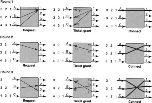
To see this algorithm in action, consider Figure 13.6, where in the top frame, input line card A has three packets destined to outputs 1, 2, and 3, respectively. B has three similar packets destined to the same outputs, while C has packets destined to outputs 1, 3, and 4. Assume the packets have the same size in this example (though this is not needed for the take-a-ticket algorithm to work).
Each input port works only on the packet at the head of its queue. Thus the algorithm begins with each input sending a request, via a control bus, to the output port to which the packet at the head of its input queue is destined. Thus in the example each input sends a request to output port 1 for permission to send a packet.
In general, a ticket number is a small integer that wraps around and is given out in order of arrival, as in a deli. In this case, assume that A’s request arrived first on the serial control bus, followed by B, followed by C, though the top left picture makes it appear that the requests are sent concurrently. Since output port 1 can service only one packet at a time, it serializes the requests, returning T1 to A, T2 to B, and T3 to C.
Thus in the middle picture of the top row, output port 1 also broadcasts the current ticket number it is serving (T1) on another control bus. When A sees it has a matching number for input 1, in the picture on the top right, A then connects its input bus to the output bus of 1 and sends its packet on its input bus. Thus by the end of the topmost row of pictures, A has sent the packet at the head of its input queue to output port 1. Unfortunately, all the other input ports, B and C, are stuck waiting to get a matching ticket number from output port 1.
The second row in Figure 13.6 starts with A sending a request for the packet that is now at the head of its queue to output port 2; A is returned a ticket number, T1, for port 2.1 In the middle picture of the second row, port 1 announces that it is ready for T2, and port 2 announces it is ready for ticket T1. This results in the rightmost picture of the second row, where A is connected to port 2 and B is connected to port 1 and the corresponding packets are transferred.
The third row of pictures in Figure 13.6 starts similarly with A and B sending a request for ports 3 and 2, respectively. Note that poor C is still stuck waiting for its ticket number, T3, which it obtained two iterations ago, to be announced by output port 1. Thus C makes no more requests until the packet at the head of its queue is served. A is returned T1 for port 3, and B is returned T2 for port 2. Then port 1 broadcasts T3 (finally!), port 2 broadcasts T2, and port 3 broadcasts T1. This results in the final picture of the third row, where the crossbar connects A and 3, B and 2, and C and 1.
The take-a-ticket scheme scales well in control state, requiring only two (log2 N)-bit counters at each output port to store the current ticket number being served and the highest ticket number dispensed. This allowed the implementation in DEC’s Gigaswitch to scale easily to 36 ports [SKO+94], even in the early 1990s, when on-chip memory was limited. The scheme used a distributed scheduler, with each output port’s arbitration done by a so-called GPI chip per line card; the GPI chips communicate via a control bus.
The GPI chips have to arbitrate for the (serial) control bus in order to present a request to an output line card and to obtain a queue number. Because the control bus is a broadcast bus, an input port can figure out when its turn comes by observing the service of those who were before it, and it can then instruct the crossbar to make a connection.
Besides small control state, the take-a-ticket scheme has the advantage of being able to handle variable-size packets directly. Output ports can asynchronously broadcast the next ticket number when they finish receiving the current packet; different output ports can broadcast their current ticket numbers at arbitrary times. Thus, unlike all the other schemes described later, there is no header and control overhead to break up packets into “cells” and then do later reassembly. On the other hand, take-a-ticket has limited parallelism because of head-of-line blocking, a phenomenon we look at in the next section.
The take-a-ticket scheme also allows a nice feature called hunt groups. Any set of line cards (not just physically contiguous line cards) can be aggregated to form an effectively higher-bandwidth link called a hunt group. Thus three 100-Mbps links can be aggregated to look like a 300-Mbps link.
The hunt group idea requires only small modifications to the original scheduling algorithm because each of the GPI chips in the group can observe each other’s messages on the control bus and thus keep local copies of the (common) ticket number consistent. The next packet destined to the group is served by the first free output port in the hunt group, much as in a delicatessen with multiple servers. While basic hunt groups can cause reordering of packets sent to different links, a small modification allows packets from one input to be sent to only one output port in a hunt group via a simple deterministic hash. This modification avoids reordering, at the cost of reduced parallelism.
Since the Gigaswitch was a bridge, it had to handle LAN multicast. Because the take-a-ticket scheduling mechanism uses distributed scheduling via separate GPI chips per output, it is hard to coordinate all schedulers to ensure that every output port is free. Further, waiting for all ports to have a free ticket for a multicast packet would result in blocking some ports that were ready to service the packet early, wasting throughput. Hence multicast was handled by a central processor in software and was thus accorded “second-class” status.
13.5 HEAD-OF-LINE BLOCKING
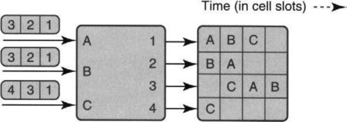
Forgetting about the internal mechanics of Figure 13.6, observe that there were nine potential transmission opportunities in three iterations (three input ports and three iterations); but after the end of the picture in the bottom right, there is one packet in B’s queue and two in C’s queue. Thus only six of potentially nine packets have been sent, thereby taking limited advantage of parallelism.
This focus on only input–output behavior is sketched in Figure 13.7. The figure shows the packets sent in each packet time at each output port. Each output port has an associated time line labeled with the input port that sent a packet during the corresponding time period, with a blank if there is none. Note also that this picture continues the example started in Figure 13.6 for three more iterations, until all input queues are empty.
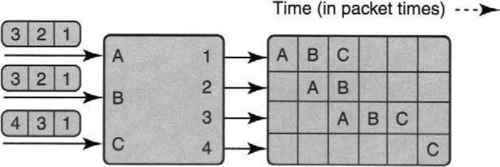
It is easy to see visually from the right of Figure 13.7 that only roughly half of the transmission opportunities (more precisely, 9 out of 24) are used. Now, of course, no algorithm can do better for certain scenarios. However, other algorithms, such as iSLIP (see Figure 13.11 in Section 13.8) can extract more parallel opportunities and finish the same nine packets in four iterations instead of six.
In the first iteration of Figure 13.7, all inputs have packets waiting for output 1. Since only one (i.e., A) can send a packet to output 1 at a time, the entire queue at B (and C) is stuck waiting for A to complete. Since the entire queue is held hostage by the progress of the head of the queue, or line, this is called head-of-line (HOL) blocking. iSLIP and PIM get around this limitation by allowing packets behind a blocked packet to make progress (for example, the packet destined for output port 2 in the input queue at B can be sent to output port 2 in iteration 1 of Figure 13.7) at the cost of a more complex scheduling algorithm.
The loss of throughput caused by HOL blocking can be analytically captured using a simple uniform-traffic model. Assume that the head of each input queue has a packet destined for each of N outputs with probability 1/N. Thus if two or more input ports send to the same output port, all but one input are blocked. The entire throughput of the other inputs is “lost” due to head-of-line blocking.
More precisely, assume equal-size packets and one initial trial where a random process draws a destination port at each input port uniformly from 1 to N. Instead of focusing on input ports, let us focus on the probability that an output port O is idle. This is simply the probability that none of the N input ports chooses O. Since each input port does not choose O with probability 1 – 1/N, the probability that all N of them will not choose O is (1 – 1/N)N. This expression rapidly converges to 1/e. Thus the probability that O is busy is 1 – 1/e, which is 0.63. Thus the throughput of the switch is not N * B, which is what it could be ideally if all N output links are busy operating at B bits per second. Instead, it is 63% of this maximum value, because 37% of the links are idle.
This analysis is simplistic and (incorrectly) assumes that each iteration is independent. In reality, packets picked in one iteration that are not sent must be attempted in the next iteration (without another random coin toss to select the destination). A classic analysis [KHM87] that removes the independent-trials assumption shows that the actual utilization is slightly worse and is closer to 58%.
But are uniform-traffic distributions realistic? Clearly, the analysis is very dependent on the traffic distribution because no switch can do well if all traffic is destined to one server port. Simple analyses show that the effect of head-of-line blocking can be reduced by using hunt groups, by using speedup in the crossbar fabric compared to the links, and by assuming more realistic distributions in which a number of clients send traffic to a few servers.
However, it should be clear that there do exist distributions where head-of-line blocking can cause great damage to throughput. Imagine that every input link has B packets to port 1, followed by B packets to port 2, and so on, and finally B packets to port N. The same distribution of input packets is present in all input ports. Thus clearly, when scheduling the group of initial packets to port 1, essentially head-of-line blocking will limit the switch to sending only one packet per input each time. Thus the switch reduces to 1/N of its possible throughput if B is large enough. On the other hand, we will see that switches that use virtual output queues (VOQs) (defined later in this chapter) can, in the same situations, achieve nearly 100% throughput. This is because in such schemes each block of B packets stays in separate queues at each input.
13.6 AVOIDING HEAD-OF-LINE BLOCKING VIA OUTPUT QUEUING
When HOL blocking was discovered, there was a slew of papers that proposed output queuing in place of input queuing to avoid HOL blocking. Suppose that packets can somehow be sent to an output port without any queuing at the input. Then it is impossible for packet P destined for a busy output port to block another packet behind it. This is because packet P is sent off to the queue at the output port, where it can only block packets sent to the same output port.
The simplest way to do this would be to run the fabric N times faster than the input links. Then even if all N inputs send to the same output in a given cell time, all N cells can be sent through the fabric to be queued at the output. Thus pure output queuing requires an N-fold speedup within the fabric. This can be expensive or infeasible.
A practical implementation of output queuing was provided by the knockout [YHA87] switch design. Suppose that receiving N cells to the same destination in any cell time is rare and that the expected number is k, which is much smaller than N. Then the expected case can be optimized (P11) by designing the fabric links to run k times as fast as an input link, instead of N. This is a big savings within the fabric. It can be realized with hardware parallelism (P5) by using k parallel buses.
Unlike the take-a-ticket scheme, all the remaining schemes in this chapter, including the knockout scheme, rely on breaking up packets into fixed-size cells. For the rest of the chapter, cells will be used in place of packets, always understanding that there must be an initial stage where packets are broken into cells and then reassembled at the output port.
Besides a faster switch, the knockout scheme needs an output queue that accepts cells k times faster than the speed of the output link. A naive design that uses this simple specification can be built using a fast FIFO but would be expensive. Also, the faster FIFO is overkill, because clearly the buffer cannot sustain a long-term imbalance between its input and output speeds. Thus the buffer specification can be relaxed (P3) to allow it to handle only short periods, in which cells arrive k times as fast as they are being taken out. This can be handled by memory interleaving and k parallel memories. A distributor (that does run k times as fast) sprays arriving cells into k memories in round-robin order, and departing cells are read out in the same order.
Finally, the design has to fairly handle the case where the expected case is violated and N > k cells get sent to the same output at the same time. The easiest way to understand the general solution is first to understand three simpler cases.
Two contenders, one winner: In the simplest case of k = 1 and N = 2, the arbiter must choose one cell fairly from two choices. This can be done by building a primitive 2-by-2 switching element, called a concentrator, that randomly picks a winner and a loser. The winner output is the cell that is chosen. The loser output is useful for the general case, in which several primitive 2-by-2 concentrators are combined.
Many contenders, one winner: Now consider when k = 1 (only one cell can be accepted) and N > 2 (there are more than two cells that the arbiter must choose fairly from). A simple strategy uses divide-and-conquer (P15, efficient data structures) to create a knockout tree of 2-by-2 concentrators. As in the first round of a tennis tournament, the cells are paired up using N/2 copies of the basic 2-by-2 concentrator, each representing a tennis match. This forms the bottom level of the tree. The winners of the first round are sent to a second round of N/4 concentrators, and so on. The “tournament” ends with a final, in which the root concentrator chooses a winner. Notice that the loser outputs of each concentrator are still ignored.
Many contenders, more than one winner: Finally, consider the general case where k cells must be chosen from N possible cells, for arbitrary values of k and N. A simple idea is to create k separate knockout trees to calculate the first k winners. However, to be fair, the losers of knockout trees for earlier trees have to be sent to the knockout trees for the subsequent places. This is why the basic 2-by-2 knockout concentrator has two outputs, one for the winner and one for the loser, and not just one for the winner. Loser outputs are routed to the trees for later positions.
Notice that if one had to choose four cells among eight choices, the simplest design would assign the eight choices (in pairs) to four 2-by-2 knockout concentrators. This logic will pick four winners, the desired quantity. While this logic is certainly much simpler than using four separate knockout trees, it can be very unfair. For example, suppose two very heavy traffic sources, S1 and S2, happen to be paired up, while another heavy source, S3, is paired up with a light source. In this case S1 and S2 would get roughly half the traffic that S3 obtains. It is to avoid these devious examples of unfairness that the knockout logic uses k separate trees, one for each position.
The naive way to implement the trees is to begin running the logic for the Position j tree strictly after all the logic for the Position j – 1 tree has completed. This ensures that all eligible losers have been collected. A faster implementation trick is explored in the exercises. Hopefully, this design should convince you that fairness is hard to implement correctly. This is a theme that will be explored again in the discussion of iSLIP.
While the knockout switch is important to understand because of the techniques it introduced, it is complex to implement and makes assumptions about traffic distributions. These assumptions are untrue for real topologies in which more than k clients frequently gang up to concurrently send to a popular server. More importantly, researchers devised relatively simple ways to combat HOL blocking without going to output queuing.
13.7 AVOIDING HEAD-OF-LINE BLOCKING BY USING PARALLEL ITERATIVE MATCHING
The main idea behind parallel iterative matching (PIM) [AOST93] is to reconsider input queuing but to retrofit it to avoid head-of-line blocking. It does so by allowing an input port to schedule not just the head of its input queue, but also other cells, which can make progress when the head is blocked. At first glance, this looks very hard. There could be a hundred thousand cells in each queue; attempting to maintain even 1 bit of scheduling state for each cell will take too much memory to store and process.
However, the first significant observation is that cells in each input port queue can be destined for only N possible output ports. Suppose cell P1 is before cell P2 in input queue X and that both P1 and P2 are destined for the same output queue Y. Then to preserve FIFO behavior, P1 must be scheduled before P2 anyway. Thus there is no point in attempting to schedule P2 before P1 is done. Thus obvious waste can be avoided (P1) by not scheduling any cells other than the first cell sent to every distinct output port.
Thus the first step is to exploit a degree of freedom (P13) and to decompose the single input queue of Figure 13.6 into a separate input queue per output at each input port in Figure 13.8. These are called virtual output queues (VOQs). Notice that the top left picture of Figure 13.8 contains the same input cells as in Figure 13.7, except now they are placed in separate queues.
The second significant observation is that communicating the scheduling needs of any input port takes a bitmap of only N bits, where N is the size of the switch. In the bitmap, a 1 in position i implies that there is at least one cell destined to output port i. Thus if each of N input ports communicates an N-bit vector describing its scheduling needs, the scheduler needs to process only N2 bits. For small N ≤ 32, this is not many bits to communicate via control buses or to store in control memories.
The communicating of requests is indicated in the top left picture of Figure 13.8 by showing a line sent from each input port to each output port for which it has a nonempty VOQ. Notice A does not have a line to port 4 because it has no cell for port 4. Notice also that input port C sends a request for the cell destined for output port 4 in input port C, while the same cell is the last cell in input queue C in the single-input-queue scenario of Figure 13.6.
What is still required is a scheduling algorithm that matches resources to needs. Although the scheduling algorithm is clever, in the author’s opinion the real breakthrough was observing that, using VOQs, input queue scheduling without HOL blocking is feasible to think about. To keep the example in Figure 13.8 corresponding to Figure 13.6, assume that every packet in the scenario of Figure 13.6 is converted into a single cell in Figure 13.8.
To motivate the scheduling algorithm used in PIM, observe that in the top left of Figure 13.8, output port 1 gets three requests from A, B, and C but can service only one in the next slot. A simple way to choose between requests is to choose randomly (P3a). Thus in the Grant phase (top middle of Figure 13.8), output port 1 chooses B randomly. Similarly, assume that port 2 randomly chooses A (from A and B), and port 3 randomly chooses A (from A, B, and C). Finally, port 4 chooses its only requester, C.
However, resolving output-port contention is insufficient because there is also input-port contention. Two output ports can randomly grant to the same input port, which must choose exactly one to send a cell to. For example, in the top middle of Figure 13.8, A has an embarrassment of riches by getting grants from outputs 2 and 3. Thus a third, Accept, phase is necessary, in which each input port chooses an output port randomly (since randomization was used in the Grant phase, why not use it again?).
Thus in the top right picture of Figure 13.8, A randomly chooses port 2. B and C have no choice and choose ports 1 and 4, respectively. Crossbar connections are made, and the packets from A to port 2, B to port 1, and C to to Port 4 are transferred. While in this case, the corresponding match found was a maximal match (i.e., cannot be improved), in some cases the random choices may result in a match that can be improved further. For example, in the unlikely event that ports 1, 2, and 3 all choose A, the match size will only be of size 2.
In such cases, although not shown it in the figure, it may be worthwhile for the algorithm to mask out all matched inputs and outputs and iterate more times (for the same forthcoming time slot). If the match on the current iteration is not maximal, a further iteration will improve the size of the match by at least 1. Note that subsequent iterations cannot worsen the match because existing matches are preserved across iterations. While the worst-case time to reach a maximal match for N inputs is N iterations, a simple argument shows that the expected number of matches is closer to log N. The DEC AN-2 implementation [AOST93] used three iterations for a 30-port switch.
Our example in Figure 13.8, however, uses only one iteration for each match. The middle row shows the second match for the second cell time, in which, for example, A and C both ask for port 1 (but not B, because the B-to-1 cell was sent in the last cell time). Port 1 randomly chooses C, and the final match is A, 3, B, 2, and C, 1. The third row shows the third match, this time of size 2. At the end of the third match, only the cell destined to port 3 in input queue B is not sent. Thus in four cell times (of which the fourth cell time is sparsely used and could have been used to send more traffic) all the traffic is sent. This is clearly more efficient than the take-a-ticket example of Figure 13.6.
13.8 AVOIDING RANDOMIZATION WITH iSLIP
Parallel iterative matching was a seminal scheme because it introduced the idea that HOL could be avoided at reasonable hardware cost. Once that was done, just as was the case when Roger Bannister first ran the mile in under 4 minutes, others could make further improvements. But PIM has two potential problems. First, it uses randomization, and it may be hard to produce a reasonable source of random numbers at very high speeds.2 Second, it requires a logarithmic number of iterations to attain maximal matches. Given that each of a logarithmic number of iterations takes three phases and that the entire matching decision must be made within a minimum packet arrival time, it would be better to have a matching scheme that comes close to maximal matches in just one or two iterations.
iSLIP is a very popular and influential scheme that essentially “derandomizes” PIM and also achieves very close to maximal matches after just one or two iterations. The basic idea is extremely simple. When an input port or an output port in PIM experiences multiple requests, it chooses a “winning” request uniformly at random, for the sake of fairness. Whereas Ethernet provides fairness with randomness, token rings do so using a round-robin pointer implemented by a rotating token.
Similarly, iSLIP provides fairness by choosing the next winner among multiple contenders in round-robin fashion using a rotating pointer. While the round-robin pointers can be initially synchronized and cause something akin to head-of-line blocking, they tend to break free and result in maximal matches over the long run, at least as measured in simulation. Thus the subtlety in iSLIP is not the use of round-robin pointers but the apparent lack of long-term synchronization among N such pointers running concurrently.
More precisely, each output (respectively input) maintains a pointer g initially set to the first input (respectively output) port. When an output has to choose between multiple input requests, it chooses the lowest input number that is equal to or greater than g. Similarly, when an input port has to choose between multiple output-port requests, it chooses the lowest output-port number that is equal to or greater than a, where a is the pointer of the input port. If an output port is matched to an input port X, then the output-port pointer is incremented to the first port number greater than X in circular order (i.e., g becomes X + 1, unless X was the last port, in which case g wraps around to the first port number).
This simple device of a “rotating priority” allows each resource (output port, input port) to be shared reasonably fairly across all contenders at the cost of 2N extra log2 N pointers in addition to the N2 scheduling state needed on every iteration.
Figures 13.9 and 13.10 show the same scenario as in Figure 13.8 (and Figure 13.6), but using a two-iteration iSLIP. Since each row is an iteration of a match, each match is shown using two rows. Thus the three rows of Figure 13.9 show the first 1.5 matches of the scenario. Similarly, Figure 13.10 shows the remaining 1.5 matches.
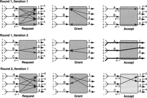
The upper left picture of Figure 13.9 is identical to Figure 13.8, in that each input port sends requests to each output port for which it has a cell destined. However, one difference is that each output port has a so-called grant pointer g, which is initialized for all outputs to be A. Similarly, each input has a so-called accept pointer called a, which is initialized for all inputs to 1.
The determinism of iSLIP causes a divergence right away in the Grant phase. Compare the upper middle of Figure 13.9 with the upper middle of Figure 13.8. For example, when output 1 receives requests from all three input ports, it grants to A because A is the smallest input greater than or equal to g1 = A. By contrast, in Figure 13.8, port 1 randomly chose input port B. At this stage the determinism of iSLIP seems a real disadvantage because A has sent requests to output ports 3 and 4 as well. Because 3 and 4 also have grant pointers g3 = g4 = A, ports 3 and 4 grant to A as well, ignoring the claims of B and C. As before, since C is the lone requester for port 4, C gets the grant from 4.
When the popular A gets three grants back from ports 1, 2, and 3, A accepts 1. This is because port 1 is the first output equal to greater than A’s accept pointer, aA, which was equal to 1. Similarly C chooses 4. Having done so, A increments aA to 2 and C increments aC to 1 (1 greater than 4 in circular order is 1). Only at this stage does output 1 increment its grant pointer, g1, to B (1 greater than the last successful grant) and port 4 similarly increments to A (1 greater than C in circular order).
Note that although ports 2 and 3 gave grants to A, they do not increment their grant pointers because A spurned their grants. If they did, it would be possible to construct a scenario where output ports keep incrementing their grant pointer beyond some input port I after unsuccessful grants, thereby continually starving input port I. Note also that the match is only of size 2; thus, unlike Figure 13.8, this iSLIP scenario can be improved by a second iteration, shown in the second row of Figure 13.9. Notice that at the end of the first iteration the matched inputs and outputs are not connected by solid lines (denoting data transfer), as shown at the top right of Figure 13.8. This data transfer will await the end of the final (in this case second) iteration.
The second iteration (middle row of Figure 13.9) starts with only inputs unmatched on previous iterations (i.e, B) requesting and only to hitherto unmatched outputs. Thus B requests to 2 and 3 (and not to 1, though B has a cell destined for 1 as well). Both 2 and 3 grant B, and B chooses 2 (the lowest one that is greater than or equal to its accept pointer of 1). One might think that B should increment its accept pointer to 3 (1 plus the last accepted, which was 2). However, to avoid starvation iSLIP does not increment pointers on iterations other than the first, for reasons that will be explained.
Thus even after B is connected to 2, 2’s grant pointer remains at A and 2’s accept pointer remains at 1. Since this is the final iteration, all matched pairs, including pairs, such as A, 1, matched in prior iterations, are all connected and data transfer (solid lines) occurs.
The third row provides some insight into how the initial synchronization of grant and accept pointers gets broken. Because only one output port has granted to A, that port (i.e., 1) gets to move on and this time to provide priority to ports beyond A. Thus even if A had a second packet destined for 1 (which it does not in this example), 1 would still grant to B.
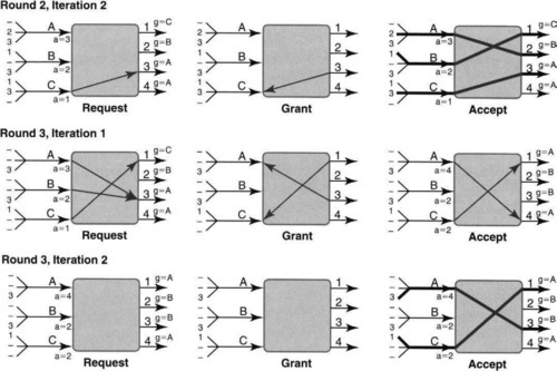
The remaining rows in Figure 13.9 and Figure 13.10 should be examined carefully by the reader to check for the updating rules for the grant and accept pointers and to check which packets are switched at each round. The bottom line is that by the end of the third row of Figure 13.10 the only cell that remains to be switched is the cell from B to 3. This can clearly be done in a fourth cell time.
Figure 13.11 shows a summary of the final scheduling (abstracting away from internal mechanics) of the iSLIP scenario and should be compared in terms of scheduling density with Figure 13.7. While these are just isolated examples, they do suggest that iSLIP (and similarly PIM) tends to waste fewer slots by avoiding head-of-line blocking. Note that both iSLIP and PIM finish the same input backlog in four cell times, as opposed to six.
Note also that when we compare Figure 13.9 with Figure 13.8, iSLIP looks worse than PIM, because it required two iterations per match for iSLIP to achieve the same match sizes as PIM does using one iteration per match. However, this is more illustrative of the startup penalty that iSLIP pays rather than a long-term penalty. In practice, as soon as the iSLIP pointers desynchronize, iSLIP does very well with just one iteration, and some commercial implementations use just one iteration: iSLIP is extremely popular.
One might summarize iSLIP as PIM with the randomization replaced by round-robin scheduling of input and output pointers. However, this characterization misses two subtle aspects of iSLIP.
• Grant pointers are incremented only in the third phase, after a grant is accepted: Intuitively, if O grants to an input port I, there is no guarantee that I will accept. Thus if O were to increment its grant pointer beyond O, it can cause traffic from I to O to be persistently starved. Even worse, McKeown et al. [Mea97] show that this simplistic round-robin scheme reduces the throughput to just 63% (for Bernoulli arrivals) because the pointers tend to synchronize and move in lockstep.
• All pointers are incremented only after the first iteration accept is granted: Once again, this rule prevents starvation, but the scenario is more subtle, which the Exercises will ask you to figure out.
Thus matches on iterations other than the first in iSLIP are considered a “bonus” that boosts throughput without being counted against a port’s quota.
13.8.1 Extending iSLIP to Multicast and Priority
iSLIP can be extended to handle priorities and multicast traffic.
PRIORITIES
Priorities are useful to send mission-critical or real-time traffic more quickly through the fabric. For example, the Cisco GSR allows voice-over-IP traffic, to be scheduled at a higher priority than other traffic, because it is rate limited and hence cannot starve other traffic.
The Tiny Tera implementation handles four levels of priorities; thus each input port has 128 VOQs (one for each combination of 32 outputs and four priority levels). Thus each input port supplies to the scheduler 128 bits of control input.
The iSLIP algorithm is modified very simply to handle priorities. First, each output port keeps a separate grant pointer gk for priority level k, and each input port keeps a separate accept pointer ak for each priority level k. In essence, the iSLIP algorithm is performed, with each entity (input port, output port) performing the iSLIP algorithm on the highest-priority level among inputs it sees.3
More precisely, each output port grants for only the highest-priority requests it receives; similarly, each input port accepts only the highest-priority grant it receives. Notice that an input port I may make a request at priority level 1 for output 5 and a request at priority level 2 for output 6 because these are the highest-priority requests the port had for outputs 5 and 6. If both outputs 5 and 6 grant to I, I does not choose between them based on accept pointers because they are at different priorities; instead I chooses the highest-priority grant. On an accept in the first iteration for priority k between input I and output port O, the priority-k accept pointer at I and the priority-k grant pointer at O are incremented.
MULTICAST
Because of applications such as video conferencing and protocols such as IP multicast, in which routers replicate packets to more than one output port, supporting multicast in switches as a first-class entity is becoming important. Recall that the take-a-ticket scheme described earlier handled multicast as a second-class entity by sending all multicast traffic to a central entity (or entities) that then sent the multicast traffic on a packet-by-packet basis to the corresponding outputs. The take-a-ticket mechanism wastes switch resources (control bandwidth, ports) and provides lower performance (larger latency, less throughput) for multicast.
On the other hand, Figure 13.4 shows that the data path of a simple crossbar switch easily supports multicasting. For example, if Input 1 in Figure 13.4 sends a message on its input bus and the crosspoints are connected so that Input 1’s bus is connected to the vertical output buses of Outputs 2 and 3, then Outputs 2 and 3 receive a copy of the packet (cell) at the same time. However, with variable-size packets, the take-a-ticket distributed-control mechanism must choose between waiting for all ports to free up at the same time and sending packets one by one.
The iSLIP extension for multicast, called ESLIP, accords multicast almost the same status as unicast. Ignoring priorities for the moment, there is one additional multicast queue per input. While to avoid HOL blocking one would ideally like a separate queue for each possible subset of output ports, that would require an impractical number of queues (216 for 16 ports). Thus multicast uses only one queue and, as such, is subject to some HOL blocking because a multicast packet cannot begin to be processed unless the multicast packets ahead of it are sent.
Suppose input I has packets for outputs O1, O2, and O3 at the head of I’s multicast queue. I is said to have a fanout of 3. Unlike in the unicast case, ESLIP maintains only a shared multicast grant pointer and no multicast accept pointer at all, as opposed to separate grant and accept pointers per port. Note that the use of a shared pointer implies a centralized implementation, unlike the take-a-ticket scheduler. As shown later, the shared pointer allows the entire switch to favor a particular input so that it can complete its fanout completely rather than have several input ports send small portions of their multicast fanout at the same time.
Thus in the example I will send a multicast request to O1, O2, and O3. But output ports like O2 may also receive unicast requests from other input ports, such as J. How should an output port balance between multicast and unicast packets? ESLIP does so by giving multicast and unicast traffic higher priority in alternate cell slots. For example, in odd slots O2 may choose unicast over multicast, and vice versa in even slots.
To continue our example, assume an odd time slot and assume that O2 has unicast traffic requests while O1 and O3 have no unicast requests. Then O2 will send a unicast grant, while O1 and O3 will send multicast grants. O1 and O3 choose the input to grant to as the first port greater than or equal to the current shared multicast grant pointer, G. Assume that I is chosen, and so O2 and O3 send multicast grants to I. Unlike unicast, I can accept all its multicast grants.
However, unlike unicast scheduling, the grant pointer for multicast is not incremented to 1 past I until I completes its fanout. Thus on the next cell slot, when the priority is given to multicast, I will be able to transmit to O2. At that point, the fanout is completed, the multicast grant pointer increments to I + 1, and the scheduler sends back a bit to I saying that the head of its multicast queue has finished transmission so the next multicast packet can be worked on. Notice that a single multicast is not necessarily completed in a single cell slot (which would require all concerned outputs to be free), but by using fanout splitting across several slots.
Clearly, iSLIP can incur HOL blocking for multicast. Specifically, if the head of the multicast queue P1 is destined for outputs O1 and O2 and both outputs are busy, but the next packet P2 is destined for O3 and O4 and both are idle, P2 must wait for P1. It would be much more difficult to implement fanout splitting for packets other than the head of the queue. Once again, this is because one cannot afford to keep a separate VOQ for each possible combination of output-port destinations.
The final ESLIP algorithm, which combines four levels of priority as well as multicasting, is described somewhat tersely in McKeown [McK97]. It is implemented in Cisco’s GSR router.
13.8.2 iSLIP Implementation Notes
The heart of the hardware implementation of iSLIP is an arbiter that chooses between N requests (encoded as a bitmap) to find the first one greater than or equal to a fixed pointer. This is what in Chapter 2 is called a programmable priority encoder; that chapter also described an efficient implementation that is nearly as fast as a priority encoder. Switch scheduling can be done by one such grant arbiter for every output port (to arbitrate requests) and one accept arbiter for every input port (to arbitrate between grants). Priorities and multicast are retrofitted into the basic structure by adding a filter on the inputs before it reaches the arbiter; for example, a priority filter zeroes out all requests except those at the highest-priority level.
Although in principle the unicast schedulers can be designed using a separate chip per port, the state is sufficiently small to be handled by a single scheduler chip with control wires coming in from and going to each of the ports. Also, the multicast algorithm requires a shared multicast pointer per priority level, which also implies a centralized scheduler. Centralization, however, implies a delay, or latency, to send requests and decisions from the port line cards to and from the central scheduler.
To tolerate this latency, the scheduler [GM99a] works on a pipeline of m cells (8 in Tiny Tera) from each VOQ and n cells (5 in Tiny Tera) from each multicast queue. This in turn implies that each line card in the Tiny Tera must communicate 3 bits per unicast VOQ denoting the size of the VOQ, up to a maximum of 8. With 32 outputs and four priority levels, each input port has to send 384 bits of unicast information. Each line card also communicates the fanout (32 bits per fanout) for each of five multicast packets in each of four priority levels, leading to 640 bits. The 32 * 1024 total bits of input information is stored in on-chip SRAM. However, for speed the information about the heads of each queue (smaller state, for example, only 1 bit per unicast VOQ) is stored in faster but less dense flip-flops.
Now consider handling multiple iterations. Note that the request phase occurs only on the first iteration and needs to be modified only on each iteration by masking off matched inputs. Thus K iterations appear to take at least 2K time steps, because the grant and accept steps of each iteration take one time step. At first glance, the architecture appears to specify that the grant phase of iteration k + 1 be started after the accept phase of iteration k. This is because one needs to know whether an input port I has been accepted in iteration k so as to avoid doing a grant for such an input in iteration k + 1.
What makes partial pipelining possible is a simple observation [GM99a]: If input I receives any grant in iteration k, then I must accept exactly one and so be unavailable in iteration k + 1. Thus the implementation specification can be relaxed (P3) to allow the grant phase of iteration k + 1 to start immediately after the grant phase of iteration k, thus overlapping with the accept phase of iteration k. To do so, we simply use the OR of all the grants to input I (at the end of iteration k) to mask out all of I’s requests (in iteration k + 1).
This reduces the overall completion time by nearly a factor of 2 time steps for k iterations—from 2k to k + 1. For example, the Tiny Tera iSLIP implementation [GM99a] does three iterations of iSLIP in 51 nsec (roughly OC-192 speeds) using a clock speed of 175 MHz; given that each clock cycle is roughly 5.7 nsec, iSLIP has nine clock cycles to complete. Since each grant and accept step takes two clock cycles, the pipelining is crucial in being able to handle three iterations in nine cycles; the naive iteration technique would have taken at least 12 clock cycles.
13.9 SCALING TO LARGER SWITCHES
So far this chapter has concentrated on fairly small switches that suffice to build up to a 32-port router. Most Internet routers deployed up to the point of writing have been in this category, sometimes for good reasons. For instance, building wiring codes tend to limit the number of offices that can be served from a wiring closet. Thus switches for local area networks [SP94] located in wiring closets tend to be well served with small port sizes.
However, the telephone network has generally employed a few very large switches that can switch 1000–10,000 lines. Employing larger switches tends to eliminate switch-to-switch links, reducing overall latency and increasing the number of switch ports available for users (as opposed to being used to connect to other switches). Thus, while a number of researchers (e.g., Refs. Tur97 and CFFT97) have argued for such large switches, there was little large-scale industrial support for such large switches until recently.
There are three recent trends that favor the design of large switches.
1. DWDM: The use of dense wavelength-division multiplexing (DWDM) to effectively bundle multiple wavelengths on optical links in the core will effectively increase the number of logical links that must be switched by core routers.
2. Fiber to the home: There is a good chance that in the near future even homes and offices will be wired directly with fiber that goes to a large central office-type switch.
3. Modular, multichassis routers: There is increasing interest in deploying router clusters, which consist of a set of routers interconnected by a high-speed network. For example, many network access points connect up routers via an FDDI link or by a Gigaswitch (see Section 13.4). Router clusters, or multichassis routers as they are sometimes called, are becoming increasingly interesting because they allow incremental growth, as explained later.
The typical lifetime of a core router is estimated [Sem02] to be 18–24 months, after which traffic increases often cause ISPs to throw away older-generation routers and wheel in new ones. Multichassis routers can extend the lifetime of a core router to 5 years or more, by allowing ISPs to start small and then to add routers to the cluster according to traffic needs.
Thus at the time of writing, Juniper Networks led the pack by announcing its T-series routers, which allow up to 16 single-chassis routers (each of which has up to 16 ports) to be assembled via a fabric into what is effectively a 256-port router. At the heart of the multichassis system is a scalable 256-by-256 switching system. Cisco Networks has recently announced its own version, the CRS-1 Router.
13.9.1 Measuring Switch Cost
Before studying switch scaling, it helps to understand the most important cost metrics of a switch. In the early days of telephone switching, crosspoints were electromagnetic switches, and thus the N2 crosspoints of a crossbar were a major cost. Even today this is a major cost for very large switches of size 1000. But because crosspoints can be thought of as just transistors, they take up very little space on a VLSI die.4
The real limits for electronic switches are pin limits on ICs. For example, given current pin limits of around 1000, of which a large number of pins must be devoted to other factors, such as power and ground, even a single bit slice of a 500-by-500 switch is impossible to package in a single chip. Of course one could multiplex several crossbar inputs on a single pin, but that would slow down the speed of each input to half the I/O speed possible on a pin.
Thus while the crossbar does indeed require N2 crosspoints (and this indeed does matter for large enough N), for values of N up to 200, much of the crosspoint complexity is contained within chips. Thus one places the largest crossbar one can implement within a chip and then one interconnects these chips to form a larger switch. Thus the dominant cost of the composite switch is the cost of the pins and the number of links between chips. Since these last two are related (most of the pins are for input and output links), the total number of pins is a reasonable cost measure. More refined cost measures take into account the type of pins (backplane, chip, board, etc.) because they have different costs.
Other factors that limit the building of large monolithic crossbar switches are the capacitive loading on the buses, scheduler complexity, and issues of rack space and power. First, if one tries to build a 256-by-256 switch using the crossbar approach of 256 input and output buses, the loading will probably result in not meeting the speed requirements for the buses. Second, note that centralized algorithms, such as iSLIP, that require N2 bits of scheduling state will not scale well to large N.
Third, many routers are limited by availability requirements to placing only a few (often one) ports in a line card. Similarly, for power and other reasons, there are often strict requirements on the number of line cards that can be placed in a rack. Thus a router with a large port count is likely to be limited by packaging requirements to use a multirack, multichassis solution consisting of several smaller fabrics connected together to form a larger, composite router. The following subsections describe strategies for doing just this.
13.9.2 Clos Networks for Medium-Size Routers
Despite the lack of current focus on crosspoints in VLSI technology, our survey of scalable fabrics for routers begins by looking at the historically earliest proposal for a scalable switch fabric. Charles Clos first proposed his idea in 1955 to reduce the expense of electromechanical switching in telephone switches. Fortunately, the design also reduces the number of components and links required to connect up a number of smaller switches. It is thus useful in a present-day context. Specifically, a Clos network appears to be used in the Juniper Networks T-series multichassis router product, introduced 47 years later, in 2002.
The basic Clos network uses a simple divide-and-conquer (P15) approach to reducing crosspoints by switching in three stages, as shown in Figure 13.12. The first stage divides the N total inputs into groups of n inputs each, and each group of n inputs is switched to the second stage by a small (n-by-k) switch. Thus there are N/n “small” switches in the first stage.
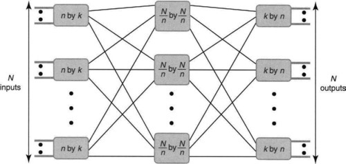
The second stage consists of k switches, each of which is an N/n-by-N/n switch. Each of the k outputs of each first-stage switch is connected in order to all the k second-stage switches. More precisely, output j of switch i in the first stage is connected to input i of switch j in the second stage. The third stage is a mirror reversal of the first stage, and the interconnections between the second and third stages are also the mirror reversal of those between the first and second stages. The view from outputs leftward to the middle stage is the same as the view from inputs to the middle stage. More precisely, each of the N/n outputs of the first stage is connected in order to the inputs of the third stage.
A switch is said to be nonblocking if whenever the input and output are free, a connection can be made through the switch using free resources. Thus a crossbar is always nonblocking by selecting the crosspoint corresponding to the input–output pair, which is never used for any other pair. On the other hand, in Figure 13.12, every input switch has only k connections to the middle stage, and every middle stage has only one path to any particular switch in the third stage. Thus, for small k it is easily possible to block a new connection because there is no path from an input / to a middle-stage switch that has a free line to an output O.
CLOS NETWORKS IN TELEPHONY
Clos’s insight was to see that if k ≥ 2n − 1, then the resulting Clos network could indeed simulate a crossbar (i.e., is nonblocking) while still reducing the number of crosspoints to be ![]() instead of N2. This can be a big savings for large N. Of course, to achieve this crosspoint reduction, the Clos network has increased latency by two extra stages of switching delay, but that is often acceptable.
instead of N2. This can be a big savings for large N. Of course, to achieve this crosspoint reduction, the Clos network has increased latency by two extra stages of switching delay, but that is often acceptable.
The proof of Clos’s theorem is easy to see from Figure 13.13. If a hitherto-idle input i wishes to be connected to an idle output o, then consider the first-stage switch S that I is busy new connected to. There can be at most n – 1 other inputs in S that are busy (S is an n-by-k switch). These n – 1 busy input links of S can be connected to at most n – 1 middle-stage switches.
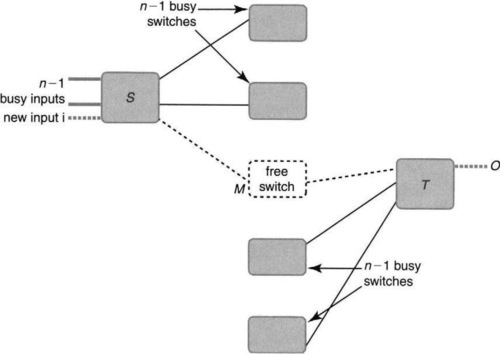
Similarly, focusing on output o, consider the last-stage switch T that o is connected to. Then T can have at most n – 1 other outputs that are busy, and each of these outputs can be connected via at most n – 1 middle-stage switches. Since both S and T are connected to k middle-stage switches, if k ≥ 2n – 1, then it is always possible to find a middle-stage switch M that has a free input link to connect to S and a free output link to connect to T. Since S and T are assumed to be crossbars or otherwise nonblocking switches, it is always possible to connect i to the corresponding input link to M and to connect the corresponding output link of M to o.
If k = 2n – 1 and n is set to its optimal value of ![]() , then the number of crosspoints (summed across all smaller switches in Figure 13.12) becomes
, then the number of crosspoints (summed across all smaller switches in Figure 13.12) becomes ![]() . For example, for N = 512, this reduces the number of crosspoints from 4.2 million for a crossbar to 516,096 for a three-stage Clos switch. Larger telephone switches, such as the No. 1. ESS, which can handle 65,000 inputs, use an eight-stage switch for further reductions in crosspoint size.
. For example, for N = 512, this reduces the number of crosspoints from 4.2 million for a crossbar to 516,096 for a three-stage Clos switch. Larger telephone switches, such as the No. 1. ESS, which can handle 65,000 inputs, use an eight-stage switch for further reductions in crosspoint size.
CLOS NETWORKS AND MULTICHASSIS ROUTERS
On the other hand, for networking using VLSI switches, what is important is the total number of switches and the number of links interconnecting switches. Recall that the largest possible switches are fabricated in VLSI and that their cost is a constant, regardless of their crosspoint size. Juniper Networks, for example, uses a Clos network to form effectively a 256-by-256 multichassis router by connecting sixteen 16-x-16 T-series routers in the first stage.
Using a standard Clos network for a fully populated multichassis router would require 16 routers in the first stage, 16 in the third stage, and k = 2 * 16 – 1 = 31 switches in the middle stage. Clearly, Juniper can (and does) reduce the cost of this configuration by setting k = n. Thus the Juniper multichassis router requires only 16 switches in the middle stage.
What happens to a Clos network when k reduces from 2n – 1 to n? If k = n, the Clos network is no longer nonblocking. Instead, the Clos network becomes what is called rearrangeably nonblocking. In other words, the new input i can be connected to o as long as it’s possible to rearrange some of the existing connections between inputs and outputs to use different middle-stage switches. A proof and possible switching algorithm is described in the Appendix. It can be safely skipped by readers uninterested in the theory.
The bottom line behind all the math in Section A.3.1 in the Appendix is as follows. First, k = n is clearly much more economical than k = 2n – 1 because it reduces the number of middle-layer switches by a factor of 2. However, while the Clos network is rearrangably nonblocking, deterministic edge-coloring algorithms for switch scheduling appear at this time to be quite complex. Second, the matching proof for telephone calls assumes that all calls appear at the inputs at the same time; when a new call arrives, existing calls have to be potentially rearranged to fit the new routes. So what does Juniper Networks do when faced with this potential choice between economy (k = n) and complexity (for edge coloring and rearrangement)?
While it’s not possible to be sure about what Juniper actually does, because their documentation is (probably intentionally) vague, one can hazard some reasonable guesses. First, it is clear they finesse the whole issue of rearrangement by replacing calls with packets and packets by fixed-size cells within the fabric. Thus in each cell time, cells appear at each input destined to every output; each new cell time requires a fresh application of the matching algorithm, unfettered by the past. Second, their documentation indicates that in place of doing a slow, perfect job using edge coloring, they do a reasonable, but perhaps imperfect, job by distributing the traffic of each input across the middle switches using some form of load balancing.
The Juniper documentation claims that “dividing packets into cells and then distributing them across the Clos fabric achieves the same effect as moving connections in a circuit-switched network because all the paths are used simultaneously.” While this is roughly right in a long-term sense, simple deterministic algorithms (in which each input chooses the middle switch to send its next cell in round-robin order; see Exercises) can lead to hot spots in terms of congested middle switches.
Thus it may be that the actual algorithm is deterministic and has possible cases of long-term congestion (which can then be brushed aside by marketing as being pathological). However, it may also be that the actual algorithm is randomized. In the simplest version, each input switch picks a random middle switch (P3a) for each cell it wishes to transmit.
In a formal probabilistic sense, the expected number of cells each middle switch will receive will be N/n, which is exactly the number of output links each middle switch has. Thus if there is a stream of cells going to distinct outputs,5 the switch fabric can be expected to achieve 100% throughput in the expected case.
However, randomization is trickier to implement than it may sound. First, just as with hash functions, there is a reasonable probability of “collisions,” where too many input switches choose the same output switch. This can reduce throughput and may require buffering within the switch (or a two-phase process in which inputs make requests to middle switches before sending cells).
The reduced throughput can, of course, be compensated for by using a standard industry trick: speeding up internal switch links slightly. Although not given adequate attention in this chapter, speedup is a very important technique in real switches to allow simple designs while retaining efficiency.
Second, one has to find a good way to implement the randomization. Fortunately, while there are many poor implementations in existing products, there are, in fact, some excellent hardware random number generators. One good choice [All02] is the Tausworth [L’E96] random number generator. It can be implemented easily using three linear feedback shift registers (LFSRs; see Chapter 9) that are XOR’ed together. Despite its compact implementation, Tausworth passes many sophisticated tests for randomness, such as the diehard test [Mar02].
Third, the algorithms to reassemble cells into packets may be more complex when using randomized load balancing than with deterministic load balancing; in the latter case, the reassembly logic knows where to expect the next packet from.
13.9.3 Benes Networks for Larger Routers
Just as the No. 1. ESS telephone switch switches 65,000 input links, Turner [Tur97, CFFT97] has made an eloquent case that the Internet should (at least eventually) be built of a few large routers instead of several smaller routers. Such topologies can reduce the wasted links for router-to-router connections between smaller routers and thus reduce cost; they can also reduce the worst-case end-to-path length, reducing latency and improving user response times.
Essentially, a Clos network has roughly ![]() scaling, in terms of crosspoint complexity using just three stages. This trade-off and general algorithmic experience (P15) suggest that one should be able to get N log N crosspoint complexity while increasing the switch depth to log N. Such switching networks are indeed possible and have been known for years in theory, in telephony, and in the parallel computing industry. Alternatives, such as Butterfly, Delta, Banyan, and Hypercube networks, are well-known contenders.
scaling, in terms of crosspoint complexity using just three stages. This trade-off and general algorithmic experience (P15) suggest that one should be able to get N log N crosspoint complexity while increasing the switch depth to log N. Such switching networks are indeed possible and have been known for years in theory, in telephony, and in the parallel computing industry. Alternatives, such as Butterfly, Delta, Banyan, and Hypercube networks, are well-known contenders.
While the subject is vast, this chapter concentrates only on the Delta and Benes networks. Similar networks are used in many implementations. For example, the Washington University Gigabit switch [CFFT97] uses a Benes network, which can be thought of as two copies of a Delta network. Section A.4 in the Appendix outlines the (often small) differences between Delta networks and others of the same ilk.
The easiest way to understand a Delta network is recursively. Imagine that there are N inputs on the left and that this problem is to be reduced to the problem of building two smaller (N/2)-size Delta networks. To help in this reduction, assume a first stage of 2-by-2 switches. A simple scheme (Figure 13.14) is to inspect the output that every input wishes to speak to. If the output is in the upper half (MSB of output is 0), then the input is routed to the upper N/2 Delta Network; if the output is in the lower half (i.e., MSB = 1), the input is routed to the lower N/2 Delta network.
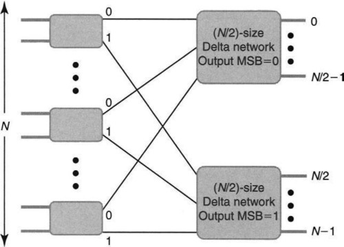
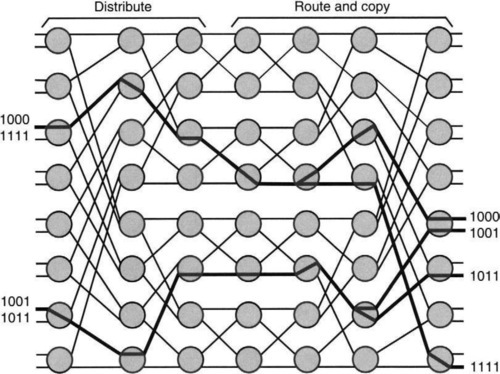
To economize on the first stage of two-input switches, group the inputs into consecutive pairs, each of which shares a two-input switch, as in Figure 13.14. Thus if the two input cells in a pair are going to different output halves, they can be switched in parallel; otherwise, one will be switched and the other is either dropped or buffered. Of course, the same process can be repeated recursively for both of the smaller (N/2)-size Delta networks, breaking them up into a layer of 2-by-2 switches followed by four N/4 switches, and so on. The complete expansion of a Delta network is shown in the first half of Figure 13.15. Notice how the recursive construction in Figure 13.14 can be seen in the connections between the first and second stages in Figure 13.15.
Thus to reduce the problem to 2 × 2 switches takes log N stages; since each stage has N/2 crosspoints, the binary Delta network has N log N crosspoint and link complexity. Clearly, we can also construct a Delta network by using d-by-d switches in the first stage and breaking up the initial network into d Delta networks of size N/d each. This reduces the number of stages to logdN and link complexity to n logd N. Given VLSI costs, it is cheaper to construct a switching chip with as large a value of d as possible to reduce link costs.
The Delta network, as do many of its close relatives (see Section A.4) such as the Banyan and the Butterfly, has a nice property called the self-routing property. For a binary Delta network, one can find the unique path from a given input to a given output o = o1, o2,… os expressed in binary by following the link corresponding to the value of oi in stage i. This should be clear from Figure 13.14, where we use the MSB at the first stage, the second bit at the second stage, and so on. For d ≥ 2, write the output address as a radix-d number, and follow successive digits in a similar fashion.
An interesting property that one can intuitively see in Figure 13.14 is that the Delta network is reversible. It is possible to trace a path from an output to an input by following bits of the input in the same way. Thus in Figure 13.14 notice that in going from outputs to inputs, the next-to-last bit of the input selects between two consecutive first-stage switches, and the last bit selects the input. This reversibility property is important because it allows the use of a mirror-reversed version of the Delta (see second half of Figure 13.15) with similar properties as the original Delta.
One problem with the Delta network is congestion. Since there is a unique path from each input to each output, the Delta network is emphatically not a permutation network. For example, if each successive pair of inputs wishes to send a cell to the same output half, only half of the cells can proceed to second stage; if this repeats, only a quarter can proceed to the third stage; and so on. Thus there are combinations of output requests for which the Delta network throughput can reduce to that of one link, as opposed to N links.
Clearly, one way to make the Delta network less susceptible to congestion for arbitrary permutations of input requests is to add more paths between an input and an output. Generalizing the ideas in a Clos network (Figure 13.12), one can construct a Benes network (Figure 13.15), which consists of two (log N)-depth networks: The left half is a standard Delta network, and the right half is a mirror-reversed Delta network. Look at the right half backwards, going left from the outputs: Notice that the connections from the last stage to the next-to-last stage are identical to those between the first and second stages.
One can also visualize a Benes network recursively (P15) by extending Figure 13.14 by adding a third stage of 2-by-2 switches and by connecting these third stages to the two (N/2)-sized networks in the middle in the same way as the first-stage switches are connected to the two middle (N/2)-sized networks (Figure 13.16). Observe that this recursion can be used to directly create Figure 13.15 without creating two separate Delta networks.
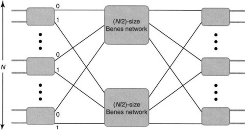
Observe the similarity between the recursive version of the Benes network in Figure 13.16 and the Clos network of Figure 13.12. This similarity can be exploited to prove that the Benes can route any permutation of output requests in a manner similar to our proof (see earlier box) of the rearrangably nonblocking property of a Clos network.
In each of two iterations, start by doing a perfect matching between the first and last stages of Figure 13.16, as before, and pick one of the two middle switches. However, rather than stopping here as in the Clos proof, the algorithm must recursively follow the same routing procedure in the (N/2)-sized Benes network. Alternatively, the whole process can be formulated using edge coloring. The final message is that it is possible to perfectly route arbitrary permutations in a Benes network; however, doing so is fairly complex and is unlikely to be accomplished cheaply in a minimum packet arrival time.
However, recall the earlier argument that a randomized strategy works well, in an expected sense, for Clos networks instead of a more complex and deterministic edge-coloring scheme. Analagous to picking a random middle switch in the Clos network, returning to Figure 13.15 one can pick a random destination for each cell in the first half. One can then route from the random intermediate destination to the actual cell destination (using reverse Delta routing) in the second half. The roots of this idea of using random intermediate destinations go back to Valiant [Val90], who first used it to route in a (single-copy) hypercube.
As in the case of a Clos network using a random choice of middle switches, it can be shown that (in an expected sense) no internal link gets congested as long as no input or output link is congested. Intuitively, the load-splitting half takes all the traffic destined for any output link from any input and spreads it evenly over all the N output links of the first half of Figure 13.15. In the second half, because of the mirror-image structure, all the traffic of the link fans in back to the destined output links.
For example, consider the upper link coming into the first switch in the last stage of Figure 13.15. An important claim is that this upper link will carry half of the traffic to output link 1. This is because this upper link carries all the traffic destined for output link 1 from the top half of the input nodes in the route-and-copy network (mirror-reversed Delta). And by the load-splitting property of the distribute network (the first half of the Delta network), this is half of the traffic destined for output link 1. Similarly, it is possible to argue that the upper link carries half the traffic going to output link 2. Thus if output links 1 and 2 are not saturated, neither will the upper link to switch 1 in the last stage be. One can make a similar argument for any internal link in the second half.
While some of these properties of a Benes network were known before, Turner [Tur97] extended these ideas to include multicast. Notice that our previous example of a scalable switch fabric, the Juniper Clos-based multichassis router, is silent about how multicast is handled. Multicast is handled in a potentially second-class fashion using a server-based approach, as in the take-a-ticket scheme. However, in the Washington University and Growth Network switches [Tur97, CFFT97], Turner showed how to handle multicast traffic in first-class fashion. Thus his vision is for large, scalable, multimedia switches that will need to handle multicast traffic (for, say, video conferencing) as the rule rather than the exception.
To extend the Benes routing ideas to multicast, Turner starts by devising a simpler form of multicast, called copy-twice multicast. In this simpler problem, each input may specify two outputs. It is the job of the network to send two copies of the input cell to the two specified output ports. If this can be done and output links can be recycled back to inputs, then the two copies created in the first pass can be extended to four in the second pass and to 2i copies in i passes through the Benes network.
In Figure 13.15 for example, the fifth input link has a cell destined to 1000 (i.e., output 8) and to 1111 (i.e., to output 15). In the first half, the cell is randomly routed to input 7 of the second half. In the second half, follow the bits of the real outputs, MSB first, until the first point that the two output addresses differ. As usual, a 0 in the current bit is switched upward and a 1 is switched downward. Thus in the first stage of the copy network, the cell is routed to the downlink because both output addresses start with 1.
Life gets more exciting at the second stage because in the second bit from the right, the addresses differ. Thus the second-stage switch in the copy network (more precisely the fourth switch from the top) now replicates the cell in two directions. The two output paths have separated at the first differing bit. From now each of the two cells (the single cell recall is now two cells) follows the address of its corresponding output. Check that following the last two bits of 1000 and 1111 will cause the two cells to reach outputs 8 and 15 in Figure 13.15.
Because of a very similar intuition, it can be shown that doing the copy at the first differing bit does not cause any internal link to be overloaded if the output and input links are not overloaded [Tur97]. In fact, the same result would hold if a copy-3 network (i.e., a network capable of producing three copies in one pass) was used. So why stop at two?
It turns out that when a cell comes into a switch it carries a multicast output-link specifier that has to be translated into two (or more) unicast specifiers for each pass. Similarly, each cell must carry two (or more) addresses during its travels. Thus using a small number like 2 limits the complexity of the port-mapping operation and the header overhead. Using larger numbers would only decrease the number of passes to replicate a multicast cell.
One of the nice features of Turner’s multicast design is that larger multicast fanouts can be handled by multiple iterations. This can be logically pictured as a multicast binary tree (P15) across several Benes networks connected in series. Of course, in reality the same Benes network is reused, reducing the cost. However, this mental picture indicates why adding a new multicast connection is very efficient. It simply involves adding a new leaf to the tree, with a minimum of disturbance to existing multicast tree nodes or other connections [Tur97].
Thus the Turner switch tends to use resources optimally because of recycling. The design allows resources (crosspoints, mapping tables, etc.) to scale as N log N, can handle any configuration of unicast and multicast traffic, and can add or remove an endpoint from a multicast tree in constant time. Competing switch architectures fail to satisfy all these conditions, sometimes spectacularly. This means that in practice, they can handle only a very limited amount of multicast traffic. Of course, one can argue about the current importance of multicast, which is certainly limited at the time of writing. However, with the rise of videoconferencing over the Internet, one can clearly envision a future where large multimedia switches are key.
Before ending this section, it is worth noting that just as with the Clos switch, the conceptual simplicity of a randomized load-balancing strategy for a Benes network comes with some attendant implementation complexity. First, since randomized load balancing is not perfect, the Turner switch needs buffers and flow control. Second, it is important to get the randomization done right. The first prototype Washington University switch [CFFT97] used simple load balancing based on a counter. However, when this switch was redesigned as part of a company called Growth Networks [Tur02], the switch used a much more sophisticated randomizer to deal with pathological input patterns. Finally, efficient resequencing of cells takes special effort in this architecture [Tur97].
13.10 SCALING TO FASTER SWITCHES
The preceding section focused on how switches can scale in size. This section studies how switches can scale in speed. Now, it may be that the speeds of individual fiber channels level off at some point. Many pundits say that fundamental SRAM and optical limits will limit individual fiber channels to OC-768 speeds. The capacity of fiber may then be used for producing more individual channels (e.g., using multiple wavelengths) rather than higher-speed individual channels. The use of more channels then affects switching only in terms of increasing port count and can be handled using the techniques of the previous section.
While this is one viewpoint, the lessons of history should teach us that it is certainly possible for individual applications to increase their speed needs and for technology surprisingly to keep pace by producing faster link speeds that increase from 40 Gbps today to 10 terabits in, say, 5 years. Thus it is worthwhile to look for techniques to scale switches in speed. There are three common techniques: bit slicing, the use of short links, and the use of randomized memory sharing.
13.10.1 Using Bit Slicing for Higher-Speed Fabrics
The simplest way to cope with link speed increases is to use a faster clock rate to run the switching electronics. Unfortunately, optical speeds increase exponentially, while ASIC clock rates increase only at around 10% per year. However, by Moore’s law, the number of transistors placed on a chip doubles every 18–24 months without a cost increase. Thus the simplest way to cope with link speed increases is to use parallelism.
Suppose it were possible to build a crossbar where every link has speed S. Then to handle links of speed kS for some constant k, a design could use k crossbar “slices.” For every group of k bits coming from a link, one bit each is sent to each crossbar slice. Thus each slice sees a reduced link speed of kS/k = S and thus can be feasibly implemented. Of course, this implies that the reassembly logic can scale in speed.
If the bits are distributed to slices in deterministic fashion (i.e., bit 1 of the first cell goes to slice 1, bit 2 to slice 2, etc.), the reassembly logic can be simplified because it knows on which slice to expect the next bit. However, care must be taken to avoid synchronization errors. The scheduler can make the same decision for all slices, making the scheduler easy to build.
The Juniper T-series [Sem02] uses four active switch fabric planes (i.e., slices). It also uses a fifth plane as a hot-standby for redundancy. Since each plane uses a request-grant mechanism, if a grant does not return within a timeout, a plane failure can be detected. At this point, only the cells in transit within the failed plane are lost, the failed plane is swapped out for maintenance, and the standby plane is swapped in.
While little discussed so far, redundancy and fault tolerance are crucial for large switch designs because more is at stake. If a small, 8-port router fails, only a few users are affected. But a large, 256-port-by-256-port router must work nearly always, with internal redundancy, masking out faults. This is because external redundancy, in terms of a second such router, is too expensive. Most ISPs require core routers to be NEBS (Network Equipment Building System) [NEB02] compliant. Typically, large routers are expected to have at most 5 minutes of downtime in a year.
13.10.2 Using Short Links for Higher-Speed Fabrics
One feature of interconnection networks ignored so far is the physical length of the links used between stages. Links come in various forms, from serial links between chips, to backplane traces, to cable connections between different line cards. Intuitively, the length matters because long wires increase delay and decrease bit rate, unless compensated for using more expensive signaling technology, such as optical signaling.
A look at the Delta and Clos networks shows that these networks use at least a few long wires between stages, whose length scales as O(N). There are, however, interconnect networks that can be packaged with uniformly short wires. These are the so-called low-dimensional mesh networks. Such mesh networks have a checkered history in parallel computing, being used by Cray and Intel supercomputers.
The simplest low-dimensional mesh is the 1D torus, which is basically a line of nodes in which the last node is also connected to the first node to form a logical ring (Figure 13.17). A 2D torus is basically a two-dimensional grid of nodes where the last node in each row or column is also connected to the first node in the same row or column. A 3D torus is the same idea extended to a three-dimensional grid.
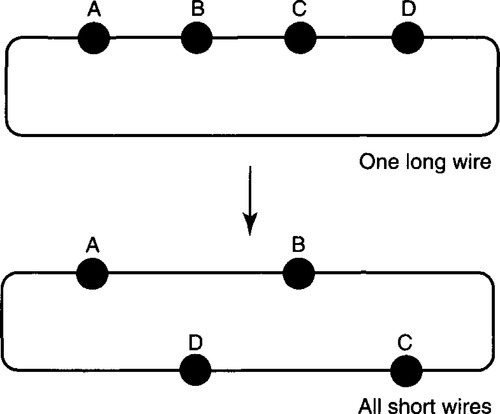
Even a 1D torus, which is logically a ring, appears to have one long wire that connects the first and last nodes (Figure 13.17). However, a clever way to amortize this long line length across all nodes is to use a simple degree of freedom (P13) and to lay out the first half of the nodes on the forward path of the ring (Figure 13.17) and the second half on the reverse path. While the length of the A-to-B wire may have doubled, there are no long wires. The same idea can be extended for 2D and 3D toruses by repeating this idea across rows and columns.
Like a Butterfly or Delta network, the problem with a 1D torus, however, is that it suffers from congestion, because there are only two paths between two inputs. It also suffers from high latency because some pairs of nodes have to travel O(N/2) hops. The congestion and latency problems are relieved by using a 3D torus. For example, in a 3D torus that is 8 by 8 by 8, an average message can choose [Dal02] between 90 paths of six hops each.
The Avici TSR Router [Dal02] is an example of a router built using a 3D torus. It can handle up to 560 line cards, and the use of short wires allows it to be packaged very neatly. A 260-line-card configuration can be packaged without any cables by connecting only adjacent backplanes using jumpers. The 560-line-card version uses one set of short cables between two rows of racks [Dal02].
Besides the use of short links, the 3D mesh offers a large number of alternate paths for fault tolerance and the ability to be incrementally upgraded with minimal extra cost. By contrast, some interconnection networks tend to require scaling in powers of 2. The Avici TSR router also handles the equivalent of head-of-line blocking by using separate virtual networks. Each virtual network uses separate buffers essentially to create the illusion of several physical switches, one of which can be used when another is blocked.
It appears that HOL blocking is handled by iSLIP, PIM, and the Avici TSR but not by the Gigaswitch, the Turner Benes network, or the Clos network. However, switches with buffered switch elements such as the Turner Benes network are not as susceptible to HOL blocking when compared to switches (such as the Gigaswitch) that do not. Given that modem switches can support thousands of cell buffers per crosspoint, HOL blocking may be a red herring for fabrics with internal buffering.
13.10.3 Memory Scaling Using Randomization
In all the switches seen so far, packets have to be stored in buffers during periods of congestion. The standard rule of thumb is for routers to have one RTT (Roundtrip Time) worth of buffering to allow congestion-control algorithms to slow down without causing packet loss. While it may be possible to get around this limit using better higher-level congestion-control algorithms, it appears that the combination of TCP and RED today requires this amount of buffering. Using 200 msec as a conservative estimate for round-trip delay, a 2-terabit router must have 0.4 terabit’s worth of packet buffers. Thus as link speeds increase, and assuming no congestion-control innovations, the memory needs will also increase.
Consider an input-buffered switch and packets coming in at OC-768 speeds. Thus a minimum-size packet arrives every 8 nsec and will require at least two accesses to memory: the first to store the packet and the second to read it out for transmission through the fabric. Given that the fastest DRAM available at the time of writing has a cycle time of 50 nsec, it is clear that the only way to meet the memory bandwidth needs using DRAM would be to use a wider memory word.
Unfortunately, one cannot use a wider memory word size than that of a minimum-size packet because it is not possible to guarantee that the next packet will be read out at the same time. One could use SRAMs (at 4-nsec cycle times at the time of writing, this should be just adequate), but then one would have to pay a cost premium of anywhere from a factor of 4 to a factor of 10.6
One way out of this dilemma is to use parallel banks of DRAMs. It is possible to keep up with link speeds using 12 DRAM banks working in parallel, each with a 40-byte access width. Intuitively, this seems plausible. For any input stream of packets, send the first packet to DRAM 1, the second to DRAM 2, etc. Unfortunately, because of QoS and scheduling algorithms, it is not clear in which order packets will be read out. Thus it may be that during some period of time all the packets are read out from a few DRAMs only, causing memory bandwidth contention and eventual packet loss.
Such memory contention problems are familiar to computer architects when using interleaved memory. For example, if an array is laid out sequentially across memory banks, it is possible that accesses that are spaced a certain stride apart (e.g., column accesses) may all hit the same bank. One potentially clever way out of the contention problem is to steal a leaf from the designers of the CYDRA-2 stride-insensitive memory [Rau91]. Their idea was to pseudo-randomly interleave storage requests to memory such that with high probability any access pattern (other than to the same word) would not cause hot spots.
In the router context, instead of sending packet 1 to DRAM 1 and so on, one would send each packet to a randomly selected DRAM. Of course, as with all randomized interleaving schemes (see the earlier Clos and Benes sections), reassembly gets more complicated, with state having to be kept (in SRAM?) to resequence these packets.
An interesting variation on this theme and that of randomized routing a la Valiant [Val90] is a technique that appears to be used by Juniper Networks in their M40 and Ml60 routers. From what is possible to glean from their patents [SAFL99], when a packet enters a line card in such a Juniper router it is (without any lookup) sent to a randomly selected other line card, where it is looked up, stored, and finally switched to its correct destination line card.
Why in the world would a leading router company go through one level of randomized indirection and take two passes though the fabric for every packet? One explanation may be that this randomization reduces the amount of required DRAM at every input line card from a “worst-case size” to a more “average size.” However, it would be nice to have some analysis or simulations to support this thesis.
13.11 CONCLUSIONS
This chapter has surveyed techniques for building switches, from small shared-memory switches to input-queued switches used in the Cisco GSR, to larger, more scalable switch fabrics used in the Juniper T130 and Avici TSR Routers.
Since this is a book about algorithmics, it is important to focus on the techniques and not get lost in the mass of product names. These are summarized in Figure 13.2. Fundamentally, the major idea in PIM and iSLIP is to realize that by using VOQs one can feasibly (with O(N2) bits) communicate all the desired communication patterns to avoid head-of-line blocking. These schemes go further and show that maximal matching can be done in N log N time using randomization (PIM) or approximately (iSLIP) using round-robin pointers per port for fairness.
While N log N is a large number, by showing that this can be done in parallel by each of N ports, the time reduces to log N (in PIM) and to a small constant (in iSLIP). Given that log N is small, even this delay can be pipelined away to run in a minimum packet time. The fundamental lesson is that even algorithms that appear complex, such as matching, can, with randomization and hardware parallelism, be made to run in a minimum packet time. Further scaling in speed can be done using bit slices.
Larger port counts are handled by algorithmic techniques based on divide-and-conquer. An understanding of the actual costs of switching shows that even a simple three-stage Clos switch works well for port sizes up to 256. However, for larger switch sizes, the Benes network, with its combination of (2log N) depth Delta networks, is better suited for the job. The main issue in both these scalable fabrics is scheduling. And in both cases, as in PIM, a complex deterministic algorithm is finessed using simple randomization. In both the Clos and Benes networks, the essential similarity of structure allows the use of an initial randomized load-balancing step followed by deterministic path selection from the randomized intermediate destination.
Similar ideas are also used to reduce memory needs by either picking a random intermediate line card or a random choice of DRAM bank to send a given packet (cell) to. The knockout switch uses trees of randomized 2-by-2 concentrators to provide k-out-of-N fairness. Thus randomization is a surprisingly important idea in switch implementations.
It is interesting to note that almost every new switch idea described in this chapter has led to a company. For example, Kanakia worked on shared-memory switches at Bell Labs and then left to found Torrent. Juniper seems to have been started with Sindhu’s idea for a new fabric based, perhaps, on the use of staging via a random intermediate line card. McKeown founded Abrizio after the success of iSLIP. Growth Networks was started by Turner, Parulkar, and Cox to commercialize Turner’s Benes switch idea, and was later sold to Cisco. Dally took his ideas for deadlock-free routing on low-dimensional meshes and moved them successfully from Cray Computers to Avici’s TSR.
Thus if you, dear reader, have an idea for a new folded Banyan or an inverted Clos, you, too, may be the founder of the next great thing in networking. Perhaps some venture capitalist will soon be meeting you in a coffee shop in Silicon Valley to make you an offer you cannot refuse.
In conclusion, for a router designer it’s better to switch than to fight—with the difficulties of designing a high-speed bus.
13.12 EXERCISES
1. Take-a-Ticket State Machine: Draw a state machine for take-a-ticket. Describe the state machine using pseudocode, with a state machine for each sender and each receiver. Extend the state machine to handle hunt groups.
2. Knockout Implementation: There are dependencies between the knockout trees. The simplest implementation passes all the losers from the Position j – 1 tree to the Position j tree. This would take k log N gate delays, because each tree takes log N gate delays. Find a way to pipeline this process such that Tree j begins to work on each batch of losers as they are determined by Tree j – 1, as opposed to waiting for all losers to be determined. Draw your implementation using 2-by-2 concentrators as your building block and estimate the worst-case delay in concentrator delays.
3. PIM unfairness: In the knockout example, using just one tree can lead to unfairness; a collection of locally fair decisions can lead to global unfairness. Surprisingly, PIM can lead to the some form of unfairness as well (but not to persistent starvation). Consider a 2-by-2 switch, where input 1 has unlimited traffic to outputs 1 and 2, and input 2 has unlimited traffic to output 1.
• Show that, on average, input 1 will get two grants from outputs 2 and 1 for half the cell slots and one grant (for output 2 only) for the remaining cell slots. What fraction of output 2’s link should input 1 receive?
• Infer, based on the preceding fraction of output 1’s bandwidth, what input 1 receives on average versus input 2. Is this fair?
4. Motivating the iSLIP Pointer Increment Rule: The following is one unfairness scenario if pointers in iSLIP are incremented incorrectly. For example, suppose in Figure 13.11 that input port A always has traffic to output ports 1, 2, and 3, whose grant pointers are initialized to A. Suppose also that input ports B and C also always have traffic to 2. Thus initially A, B, and C all grant to 1, who chooses A. In the second iteration, since input port 2 has traffic to B, 2 and B are matched.
• Suppose B increments its grant pointer to 3 based on this second iteration match. Between which port pairs can traffic be continually starved if this scenario persists?
• How does iSLIP prevent this scenario?
5. ESLIP: Answer the following questions about ESLIP.
• Describe a scenario where a multicast cell does not finish its fanout in one cycle despite the use of a shared grant pointer and the fact that multicast has priority over unicast in alternate time slots.
• Why is there no need for a shared multicast accept pointer?
6. Clos Proof Revisited: The Clos proof is based on a reduction that looks and is simple. However, until you try a few twists that do not work, you may not appreciate its simplicity. In our reduction, each iteration routed n pairs, one per input stage, using just one middle switch. Suppose instead that any set of middle switches is used that had free input and output links. Show, by counterexample, why the reduction does not work.
7. Benes Switch Load-Balancing Proof: In the Benes switch, the chapter argued that any link one hop from the output cannot be overloaded, assuming perfect load balancing at the first stage. It is helpful to work out with some simple cases to provide intuition before turning, if needed, to the proof provided in Turner [Tur97].
• Repeat the same proof for links one hop away from the network but this time for a two-copy network. Does the proof change for a three-copy network?
• Repeat all the proofs for links two hops away. Do you see a pattern that can now be stated algebraically [Tur97]?
8. Avici TSR and 3D Grid Layout: It seems a good bet that layout and packaging will be increasingly important as switches scale up in speeds. Extend the layout drawing in Figure 13.17 for a ID torus to a 2D and a 3D torus. Then read Dally [Dal02] to learn how the Avici TSR packages its 3D mesh in a box.