
Chapter 4. Fast Molecular Electrostatics Algorithms on GPUs
David J. Hardy, John E. Stone, Kirby L. Vandivort, David Gohara, Christopher Rodrigues and Klaus Schulten
In this chapter, we present GPU kernels for calculating electrostatic potential maps, which are of practical importance to modeling biomolecules. Calculations on a structured grid containing a large amount of fine-grained data parallelism make this problem especially well suited to GPU computing and a worthwhile case study. We discuss in detail the effective use of the hardware memory subsystems, kernel loop optimizations, and approaches to regularize the computational work performed by the GPU, all of which are important techniques for achieving high performance.
1
4.1. Introduction, Problem Statement, and Context
The GPU kernels discussed here form the basis for the high-performance electrostatics algorithms used in the popular software packages VMD
[1]
and APBS
[2]
.
VMD (visual molecular dynamics) is a popular software system designed for displaying, animating, and analyzing large biomolecular systems. More than 33,000 users have registered and downloaded the most recent VMD version 1.8.7. Due to its versatility and user-extensibility, VMD is also capable of displaying other large datasets, such as sequencing data, quantum chemistry data, and volumetric data. While VMD is designed to run on a diverse range of hardware — laptops, desktops, clusters, and supercomputers — it is primarily used as a scientific workstation application for interactive 3D visualization and analysis. For computations that run too long for interactive use, VMD can also be used in a batch mode to render movies for later use. A motivation for using GPU acceleration in VMD is to make slow batch-mode jobs fast enough for interactive use, which can drastically improve the productivity of scientific investigations. With CUDA-enabled GPUs widely available in desktop PCs, such acceleration can have a broad impact on the VMD user community. To date, multiple aspects of VMD have been accelerated with CUDA, including electrostatic potential calculation, ion placement, molecular orbital calculation and display, and imaging of gas migration pathways in proteins.
APBS (Adaptive Poisson-Boltzmann Solver) is a software package for evaluating the electrostatic properties of nanoscale biomolecular systems. The Poisson-Boltzmann Equation (PBE) provides a popular continuum model for describing electrostatic interactions between molecular solutes. The numerical solution of the PBE is important for molecular simulations modeled with implicit solvent (that is, the atoms of the water molecules are not explicitly represented) and permits the use of solvent having different ionic strengths. APBS can be used with molecular dynamics simulation software and also has an interface to allow execution from VMD.
The calculation of electrostatic potential maps is important for the study of the structure and function of biomolecules. Electrostatics algorithms play an important role in the model building, visualization, and analysis of biomolecular simulations; they also are an important component in solving the PBE. One often used application of electrostatic potential maps, illustrated in
Figure 4.1
, is the placement of ions in preparation for molecular dynamics simulation
[3]
.
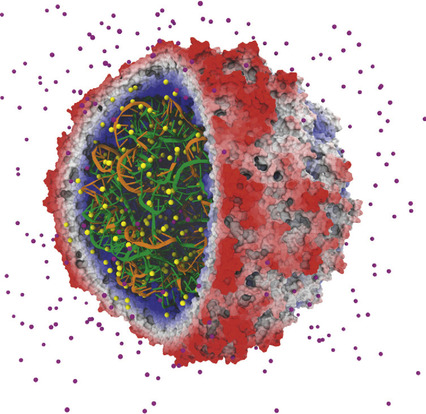 |
| Figure 4.1
An early success in applying GPUs to biomolecular modeling involved rapid calculation of electrostatic fields used to place ions in simulated structures. The satellite tobacco mosaic virus model contains hundreds of ions (sodium and chloride ions shown in light grey and dark grey, respectively) that must be correctly placed so that subsequent simulations yield correct results
[3]
. © 2009 Association for Computing Machinery, Inc. Reprinted by permission
[4]
.
|
Summing the electrostatic contributions from a collection of charged particles onto a grid of points is inherently data parallel when decomposed over the grid points. Optimized kernels have demonstrated single GPU speeds ranging from 20 to 100 times faster than a conventional CPU core.
We discuss GPU kernels for three different models of the electrostatic potential calculation: a multiple Debye-Hückel (MDH) kernel
[5]
, a simple direct Coulomb summation kernel
[3]
and a cutoff pair potential kernel
[6]
and
[7]
. The mathematical formulation can be expressed similarly for each of these models, where the electrostatic potential
 located at position
 of a uniform 3D lattice of grid points indexed by
 is calculated as the sum over
 atoms,
 in which atom
 has position
 and charge
 , and
, and
 is a constant. The function
 depends on the model; the differences in the models are significant enough as to require a completely different approach in each case to obtain good performance with GPU acceleration.
(4.1)
4.3. Algorithms, Implementations, and Evaluations
The algorithms that follow are presented in their order of difficulty for obtaining good GPU performance.
4.3.1. Multiple Debye-Hückel Electrostatics
The Multiple Debye-Hückel (MDH) method (used by APBS) calculates
Eq. 4.1
on just the faces of the 3-D lattice. For this model,
 is referred to as a “screening function” and has the form
 where
where
 is constant and
 is the “size” parameter for the
 th atom. Since the interactions computed for MDH are more computationally intensive than for the subsequent kernels discussed, less effort is required to make the MDH kernel compute bound to achieve good GPU performance.
The atom coordinates, charges, and size parameters are stored in arrays. The grid point positions for the points on the faces of the 3D lattice are also stored in an array. The sequential C implementation utilizes a doubly nested loop, with the outer loop over the grid point positions. For each grid point, we loop over the particles to sum each contribution to the potential.
The calculation is made data parallel by decomposing the work over the grid points. A GPU implementation uses a simple port of the C implementation, implicitly representing the outer loop over grid points as the work done for each thread. The arithmetic intensity of the MDH method can be increased significantly by using the GPU's fast on-chip shared memory for reuse of atom data among threads within the same thread block. Each thread block collectively loads and processes blocks of particle data
in the fast on-chip memory, reducing demand for global memory bandwidth by a factor equal to the number of threads in the thread block. For thread blocks of 64 threads or more, this enables the kernel to become arithmetic bound. A CUDA version of the MDH kernel is shown in
Figure 4.2
.
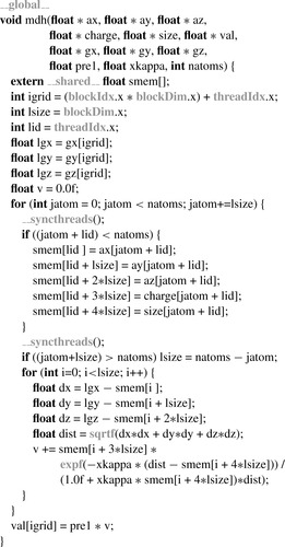 |
| Figure 4.2
In the optimized MDH kernel, each thread block collectively loads and processes blocks of atom data in fast on-chip local memory. Grey-colored program syntax denotes CUDA-specific declarations, types, functions, or built-in variables.
|
Once the algorithm is arithmetic bound, the GPU performance advantage versus the original CPU code is primarily determined by the efficiency of the specific arithmetic operations contained in the kernel. The GPU provides high-performance machine instructions for most floating-point arithmetic, so the performance gain versus the CPU for arithmetic-bound problems tends to be substantial. This is particularly true for kernels (like the MDH one given) that use special functions such as
exp()
,
which cost only a few GPU machine instructions and tens of clock cycles, rather than the tens of instructions and potentially hundreds of clock cycles that CPU implementations often require. The arithmetic-bound GPU MDH kernel provides a roughly two order of magnitude performance gain over the original C-based CPU implementation.
4.3.2. Direct Coulomb Summation
The direct Coulomb summation has
 , calculating for every grid point in the 3-D lattice the sum of the
 electrostatic contribution from each particle. The number of grid points is proportional to the number of atoms
 for a typical use case, giving
 computational complexity, although most applications require a much finer lattice resolution than the average inter-particle spacing between atoms, leading to around
 to
to
 times more grid points than atoms. A sequential algorithm would have a doubly nested loop, with the outer loop over grid points and the inner loop over the atoms. The calculation is made data parallel by decomposing the work over the grid points. A simple GPU implementation might assign each thread to calculate all contributions to a single grid point, in which case the outer loop is expressed implicitly through the parallelization, while the inner loop over atoms is explicitly executed by each thread. However, because the computational intensity of calculating each interaction is so much less than for the MDH kernel, more effort in kernel development is required to obtain high performance on the GPU.
Due to its simplicity, direct Coulomb summation provides an excellent problem for investigating the performance characteristics of the GPU hardware. We have developed and refined a collection of different kernels in an effort to achieve the best possible performance
[3]
. The particle data x/y/z/q (three coordinates and charge) is optimally stored using the
float4
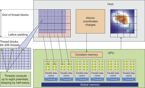
type. Since the particle data is read only and each particle is to be used by all threads simultaneously, the particles are ideally stored in the GPU constant memory. The limited size of constant memory (just 64KB with a small part of the upper portion used by the CUDA runtime libraries) means that we are able to store just up to 4000 particles. In practice, this is sufficient to adequately amortize the cost of executing a kernel on the GPU. We decompose the 3-D lattice into 2-D slices, as illustrated in
Figure 4.3
, with threads assigned to calculate the points for a given slice. The computation proceeds with multiple GPU kernel calls: for each 2-D slice of the lattice, we first zero out its GPU memory buffer, then loop over the particles by filling the constant cache with the next (up to) 4000 particles, invoke the GPU kernel to sum the electrostatic contributions to the slice, and, when finished with the loop over particles, copy the slice to the CPU.
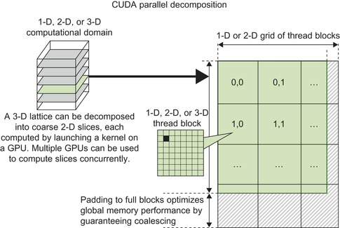 |
| Figure 4.3
Each kernel call for direct Coulomb summation operates on a 2-D slice of the 3-D lattice.
|
The CUDA thread blocks are assigned to rectangular tiles of grid points. Special cases at the edges of the lattice are avoided by padding the GPU memory buffer for each slice so that it is evenly divisible by the tile size. The padded parts of the calculation are simply discarded after copying the slice back to the CPU. Overall GPU throughput is improved by doing the additional calculations and eliminating the need for conditionals to test for the array boundary.
A simple direct Coulomb summation kernel might calculate a single grid point per thread. Each thread uses its thread and block indices to determine the spatial position of the grid point. The kernel loops over the particles stored in the constant memory cache, calculating the square of the distance between the particle and grid point, followed by a reciprocal square root function accelerated by the GPU special function unit.
Figure 4.4
shows part of this simple CUDA kernel.
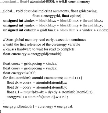 |
| Figure 4.4
A basic direct Coulomb summation GPU kernel. Atom coordinates are stored in the
|
The GPU performance is sensitive to maintaining coalesced memory reads and writes of the grid point potentials. Each kernel invocation accumulates contributions from another set of atoms, requiring
that the previously stored values be read and summed with the contributions from the new set of atoms before writing the result. Memory coalescing on earlier GPU architectures (G80 and GT200) required that a half-warp of (16) threads access an aligned, consecutive array of floats. For a 2-D slice, each half-warp-size of threads is assigned to consecutive grid points in the x-dimension.
Figure 4.4
shows the read of the previous value (curenergy
) into a register being initiated at the beginning of the kernel call, even though this previous value is not needed until the very last sum, in order to better overlap the computation with the memory access. Memory coalescing on the Fermi architecture requires access across the full warp of (32) threads. However, the performance penalty for using the earlier half-warp access is mitigated by the Fermi L1 cache.
Two different optimizations together result in more than doubling the number of interactions evaluated per second. The first optimization, shown to be of lesser benefit for GPU computation than for CPU computation, decreases arithmetic within the kernel loop by exploiting the decomposition of the 3-D lattice into slices. With planar slices taken perpendicular to the z-axis, the
 th atom has the same
 distance to every grid point
 on that slice. When buffering the particle data to send to the constant cache memory, the CPU replaces
 by
by
 , which removes a subtraction and a multiplication from each iteration of the kernel loop. Benchmarking shows a slight reduction in FLOPS on the GPU while slightly increasing the number of particle–grid interactions evaluated per second
[3]
.
, which removes a subtraction and a multiplication from each iteration of the kernel loop. Benchmarking shows a slight reduction in FLOPS on the GPU while slightly increasing the number of particle–grid interactions evaluated per second
[3]
.
The second optimization increases the ratio of arithmetic operations to memory references by calculating multiple grid points per thread, with intermediate results stored in registers. We effectively unroll the implicit outer loop over the grid points by a constant UNROLLFACTOR, reusing each atom
 read from constant memory multiple times. Unrolling in the x-dimension offers an additional reduction in arithmetic operations, with the
 's identical for the UNROLLFACTOR grid points permitting just
one necessary calculation of
's identical for the UNROLLFACTOR grid points permitting just
one necessary calculation of
 per thread. The unrolled grid points, rather than being arranged consecutively, must skip by the half-warp size in order to maintain coalesced memory reads and writes. A code fragment demonstrating the loop unrolling optimization is shown in
Figure 4.5
, illustrated by using
per thread. The unrolled grid points, rather than being arranged consecutively, must skip by the half-warp size in order to maintain coalesced memory reads and writes. A code fragment demonstrating the loop unrolling optimization is shown in
Figure 4.5
, illustrated by using
 .
.
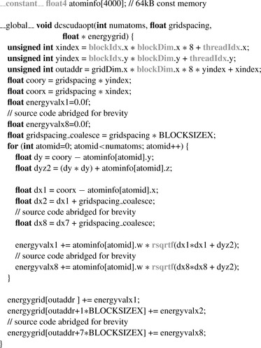 |
| Figure 4.5
Code optimizations for the direct Coulomb summation GPU kernel, using
|
Loop unrolling optimizations like the one shown here can effectively amplify memory bandwidth by moving costly memory reads into registers, ultimately trading away some amount of parallelism available in the computation. In this case, we reduce the number of thread blocks that will read each atom
 from constant memory by a factor of UNROLLFACTOR. Accordingly, the thread block tile size along the x-dimension becomes
 , which also increases the amount of data padding that might be needed along the x-dimension, and the register use-count per thread expands by almost a factor of UNROLLFACTOR. A schematic for the optimized GPU implementation is presented in
Figure 4.6
. The increased register pressure caused by unrolling can also decrease the SM occupancy that permits co-scheduling multiple thread blocks (fast context switching between the ready-to-execute warps is used to hide memory transfer latencies). The choice of unrolling factor must balance these considerations; for the direct Coulomb summation, the optimal UNROLLFACTOR is shown to be eight for both the G80 and GT200 architectures
[3]
.
, which also increases the amount of data padding that might be needed along the x-dimension, and the register use-count per thread expands by almost a factor of UNROLLFACTOR. A schematic for the optimized GPU implementation is presented in
Figure 4.6
. The increased register pressure caused by unrolling can also decrease the SM occupancy that permits co-scheduling multiple thread blocks (fast context switching between the ready-to-execute warps is used to hide memory transfer latencies). The choice of unrolling factor must balance these considerations; for the direct Coulomb summation, the optimal UNROLLFACTOR is shown to be eight for both the G80 and GT200 architectures
[3]
.
 |
| Figure 4.6
Illustration of optimized direct Coulomb summation GPU kernel.
|
The decomposition of the 3-D lattice into 2-D slices also makes it easy to support multiple GPUs. A round-robin scheduling of the slices to the available GPU devices works well for devices having equal capability, with benchmarks showing near-perfect scaling up to four GPUs
[3]
.
4.3.3. Short-Range Cutoff Electrostatics
The quadratic computational complexity of the direct Coulomb summation makes its use impractical for larger systems. Choosing a “switching” function
 that is zero beyond a fixed cutoff distance produces computational work that increases linearly in the number of particles. For molecular modeling applications, the switching function is typically chosen to be a smooth piecewise-defined polynomial.
A cutoff pair potential is often used as part of a more sophisticated method to approximate the full Coulomb interaction with
that is zero beyond a fixed cutoff distance produces computational work that increases linearly in the number of particles. For molecular modeling applications, the switching function is typically chosen to be a smooth piecewise-defined polynomial.
A cutoff pair potential is often used as part of a more sophisticated method to approximate the full Coulomb interaction with
 or
or
 computational work
[7]
.
computational work
[7]
.
A sequential algorithm for calculating a cutoff pair potential might loop over the atoms. For each atom, it is relatively easy to determine the surrounding sphere (or the enclosing cube) of grid points that are within the cutoff distance
 . The inner loop over these grid points will first test to make sure that the distance to the atom is less than the cutoff distance and will then sum the resulting interaction to the grid point potential. We always test the square of the distance against
 to avoid evaluating unnecessary square roots. This algorithm is efficient in avoiding the wasteful testing of particle–grid distances beyond the cutoff. However, disorganized memory access can still negatively impact the performance. Good locality of reference in updating the grid potentials can be maintained by performing a spatial sorting of the atoms. Since the density of biomolecules is fairly uniform, or is at least bounded, the spatial sorting is easily done by hashing the atoms into a 3-D array of fixed-size bins.
Adapting the sequential algorithm to the GPU will cause output conflicts from multiple threads, where uncoordinated concurrent memory writes from the threads are likely to produce unpredictable results. Although modern GPUs support atomic updates to global memory, this access is slower than a standard global write and much slower if there is contention between threads. The output conflicts are best eliminated by recasting the scatter memory access patterns into gather memory access patterns. Interchanging the loops produces a gather memory access pattern well suited to the GPU: each grid
point loops over the “neighborhood” of all nearby bins that are not beyond the cutoff distance from the grid point.
For GPU computation, each thread will be assigned to calculate the potential for at least one grid point. The bin neighborhood will need to surround not just the grid point(s) for the thread, but the region of grid points designated to each thread block, as depicted in
Figure 4.7
. An innermost loop over the atoms in a bin evaluates the particle–grid interaction if the pairwise distance is within the cutoff. The performance degrading impact of branch divergence, due to the conditional test of the pairwise distance within the cutoff, is improved if the threads in a warp are calculating potentials at grid points clustered together in space, making it more likely for the threads in the warp to collectively pass or fail the test condition.
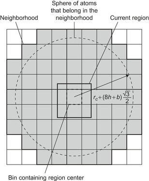 |
| Figure 4.7
Cubic region of grid points and surrounding neighborhood of atom bins. Use of small bins allows construction of a neighborhood that more tightly fits to the spherical volume defined by the cutoff distance. © 2008 Association for Computing Machinery, Inc. Reprinted by permission
[6]
.
|
Our initial effort to calculate a cutoff pair potential on the GPU adopted the direct Coulomb summation technique of storing the atom data in the GPU constant memory
[3]
, giving rise to a decomposition with coarse granularity. Use of constant memory for the atoms requires repeated kernel calls, each designed to calculate the potentials on a cubic region of grid points, but this region has to be large enough to provide a sufficient amount of work to the GPU. The CPU performs a spatial hashing of the atoms into large bins designed to form a tight-fitting neighborhood around the region of grid points, extending beyond each edge of the region by the length of the cutoff distance. Optimizations include the construction of thread blocks to arrange each half-warp of threads into the tightest possible clusters
(of
 grid points) to reduce the effects of branch divergence. The loop-unrolling optimizations were applied to keep the half-warp clusters together. Best efforts yielded speedup factors of no more than 10 due to the excessive number of failed pairwise distance tests resulting from the coarse spatial hashing.
Redesign of the GPU algorithm and data structures to use a decomposition of finer granularity, with smaller bins of atoms, ultimately resulted in more than doubling the performance over our initial effort. The CPU performs spatial hashing of atoms into bins, and then copies the bins to the GPU main memory. The thread blocks are assigned to calculate potentials for small cubic regions of grid points.
Figure 4.7
provides a 2-D schematic of the cubic region of grid points and its surrounding neighborhood of atom bins. Reducing the size of the cubic region of potentials and the volume of atom bins, from those used by the coarse granularity approach, produces a much tighter neighborhood of bins that ultimately results in a much greater success rate for the pairwise distance conditional test. Comparing the two algorithmic approaches by measuring the ratio of the volume of the
 -sphere to the volume of the enclosed cover of atoms, the success rate of the conditional test increases from about
 for the coarse granularity approach to over
 for the finer granularity approach.
Figure 4.8
illustrates the different CUDA data access patterns between the direct Coulomb summation and the two different approaches to the cutoff pair potential.
for the finer granularity approach.
Figure 4.8
illustrates the different CUDA data access patterns between the direct Coulomb summation and the two different approaches to the cutoff pair potential.
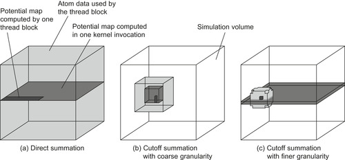 |
| Figure 4.8
Data access patterns of a CUDA grid and thread block for different potential summation implementations. The darkest shade of gray shows the subregion calculated by a single thread block, the medium gray shows the volume calculated by one kernel invocation (or, in the case of direct summation, a set of kernel invocations), and the light gray shows the data needed for calculating each thread block. © 2008 Association for Computing Machinery, Inc. Reprinted by permission
[6]
.
|
In the finer granularity approach, the threads collectively stream each bin in their neighborhood of bins to the GPU shared memory cache and then loop over the particles stored in the current cached bin to conditionally evaluate particle interactions within the cutoff distance. Indexing the bins as a 3-D
array of cubes allows the “spherical” neighborhood of bins to be precomputed as offsets from a central bin. These offsets are stored in the GPU constant memory cache and accessed optimally at near-register speed, because each consecutive offset value is read in unison by the thread block. Furthermore, there are no bank conflicts reading from the shared memory cache, because the particle data are read in unison by the thread block.
Coalesced reads and writes significantly reduce the penalty for global memory access. The smallest block size of 128 bytes for global memory coalescing determines a smallest bin depth of 8, with (8 atoms per bin)
 (4 coordinates, x/y/z/q, per atom)
 (4 bytes per coordinate)
 (128 bytes per bin). The bin side length is determined by the density of a system of particles and the expected bin-fill ratio:
 . Cubic regions of
 grid points are assigned to each thread block. The thread blocks themselves are of size
 to use an unrolling factor of
 in the y-direction, which serves to amortize the cost of caching each bin to shared memory while maximizing reuse of each particle. A code fragment for the loop over the bin neighborhood and the innermost loop over the atoms is shown in
Figure 4.9
.
in the y-direction, which serves to amortize the cost of caching each bin to shared memory while maximizing reuse of each particle. A code fragment for the loop over the bin neighborhood and the innermost loop over the atoms is shown in
Figure 4.9
.
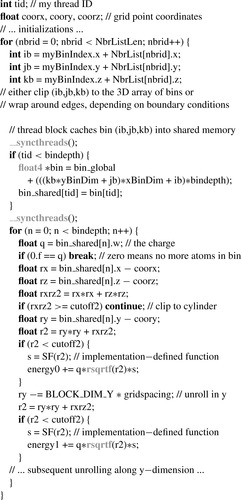 |
| Figure 4.9
Inner loops of cutoff summation kernel. Grey-colored program syntax denotes CUDA-specific declarations, types, functions, or built-in variables.
|
The grid potentials calculated by a thread block are, unlike the direct Coulomb summation kernel, accumulated in a single kernel call, which eliminates the need to read partial sums into registers. The potentials of an entire cubic region are written to global memory after completing the loop over the bin neighborhood. To achieve coalesced memory writes, the ordering of each cubic region is transposed to make the memory layout contiguous for the entire region. Upon completion of the GPU kernel calls, the CPU transposes each cubic region of potentials (skipping over the padding) into the 3-D lattice row-major ordering.
Although fixing the bin depth to eight particles optimizes global memory access, it creates a practical limit on the bin side length. Even though the density for a given molecular system is fairly uniform, it is possible for localized clustering of atoms to overfill a bin unless the bin-fill ratio is chosen to be quite small, say
 . These overfill cases are instead handled by assigning any extra particles to be calculated asynchronously by the CPU concurrently with the GPU
[6]
and
[7]
. The use of the CPU to regularize work for the GPU permits larger bin lengths that have a higher average fill, in practice using
. These overfill cases are instead handled by assigning any extra particles to be calculated asynchronously by the CPU concurrently with the GPU
[6]
and
[7]
. The use of the CPU to regularize work for the GPU permits larger bin lengths that have a higher average fill, in practice using
 , resulting in improved performance as long as the CPU finishes its computation before the GPU does. Multiple GPUs have also been employed by decomposing the 3-D lattice of grid points into slabs of cubic regions of grid points, with the slabs scheduled in parallel to the GPUs.
4.4. Final Evaluation
Performance benchmarks were run on a quiescent test platform with no windowing system, using single cores of a 2.6 GHz Intel Core 2 Extreme QX6700 quad-core CPU, as well as a 2.6 GHz Intel Xeon X5550 quad-core CPU, both running 64-bit Red Hat Enterprise Linux version 4 update 6. The CPU code was compiled using the Intel C/C
 Compiler (ICC) version 9.0. GPU benchmarks were performed using the NVIDIA CUDA programming toolkit version 3.0 running on several generations of NVIDIA GPUs.
Multiple Debye-Hückel (MDH) Electrostatics
The performance of the MDH kernel was benchmarked on CPUs, GPUs, and other accelerators, from multiple vendors, using OpenCL 1.0. When compared against the original serial X5550 SSE CPU code,
the performance increase for an IBM Cell blade (using
float16
) is 5.2
 faster, and the AMD Radeon 5870 and NVIDIA GeForce GTX 285 GPUs are 42
 faster. With further platform-specific tuning, each of these platforms could undoubtedly achieve even higher performance.
Table 4.1
summarizes the performance for OpenCL implementations of the MDH kernel using the standard OpenCL math routines.
Table 4.2
contains results for two of the GPUs, using the fast reduced precision device-native
versions of the OpenCL math routines. The greatly improved AMD Radeon 5870 results shown in
Table 4.2
clearly demonstrate the potential benefits of using the OpenCL device-native math routines in cases when precision requirements allow it. The CUDA results using device-native math routines on the GeForce GTX 480 demonstrate that well-written GPU kernels can perform very well in both the CUDA or OpenCL programming languages.
faster. With further platform-specific tuning, each of these platforms could undoubtedly achieve even higher performance.
Table 4.1
summarizes the performance for OpenCL implementations of the MDH kernel using the standard OpenCL math routines.
Table 4.2
contains results for two of the GPUs, using the fast reduced precision device-native
versions of the OpenCL math routines. The greatly improved AMD Radeon 5870 results shown in
Table 4.2
clearly demonstrate the potential benefits of using the OpenCL device-native math routines in cases when precision requirements allow it. The CUDA results using device-native math routines on the GeForce GTX 480 demonstrate that well-written GPU kernels can perform very well in both the CUDA or OpenCL programming languages.
Direct Coulomb Summation (DCS)
The performance results in
Table 4.3
compare the performance levels achieved by highly tuned CPU kernels using SSE instructions versus CUDA GPU kernels, all implemented in the C language. It is worth examining the reason for the very minimal increase in performance for the DCS kernels on the Fermi-based GeForce GTX 480 GPU as compared with the GT200-based Tesla C1060, given the significant increase in overall arithmetic performance typically associated with the Fermi-based GPUs. The reason for the rather limited increase in performance is due to the DCS kernel's performance being
bound by the execution rate for the reciprocal square root routine
rsqrtf()
. Although the Fermi GPUs are generally capable of outperforming GT200 GPUs by a factor of two on most floating-point arithmetic, the performance of the special function units that execute the machine instructions that implement
rsqrtf()
,
sin()
,
cos()
, and
exp2f()
is roughly the same as the GT200 generation of GPUs; although the effective operations per clock per multiprocessor for Fermi GPUs is double that of GT200 GPUs, the total number of multiprocessors on the device is half that of the GT200 GPUs, leading to overall DCS performance that is only slightly better than break-even with that of GT200 GPUs. Multi-GPU performance measurements were obtained by decomposing the 3-D lattice into 2-D planar slices that are then dynamically assigned to individual GPUs. Each GPU is managed by an associated CPU thread provided by the multi-GPU framework implemented in VMD
[1]
.
Short-Range Cutoff Electrostatics
The performance of the short-range cutoff electrostatic potential kernel was measured for the computation of a potential map for a
 water box containing 1,534,539 atoms, with a 0.5Å lattice spacing and a 12 Å cutoff distance. The water box was created with a volume and atom density representative of the biomolecular complexes studied during large-scale molecular dynamics simulations
[8]
and was generated using the “solvate” plugin included with VMD
[1]
. A 100-million-atom molecular dynamics simulation has been specified as a model problem for the NSF Blue Waters petascale supercomputer, creating a strong motivation for the development of molecular dynamics analysis tools capable of operating in this regime. The 1.5-million-atom test case is small enough to run in one pass on a single GPU, yet large enough to yield accurate timings and to provide performance predictions for much larger problems such as those targeting Blue Waters.
water box containing 1,534,539 atoms, with a 0.5Å lattice spacing and a 12 Å cutoff distance. The water box was created with a volume and atom density representative of the biomolecular complexes studied during large-scale molecular dynamics simulations
[8]
and was generated using the “solvate” plugin included with VMD
[1]
. A 100-million-atom molecular dynamics simulation has been specified as a model problem for the NSF Blue Waters petascale supercomputer, creating a strong motivation for the development of molecular dynamics analysis tools capable of operating in this regime. The 1.5-million-atom test case is small enough to run in one pass on a single GPU, yet large enough to yield accurate timings and to provide performance predictions for much larger problems such as those targeting Blue Waters.
CUDA benchmarks were performed on three major generations of CUDA-capable GPU devices: G80, GT200, and the Fermi architecture. The results in
Table 4.4
demonstrate the tremendous GPU speedups that can be achieved using the combination of memory bandwidth optimization techniques and the use of the CPU to optimize the GPU workload by handling exceptional work units entirely on the host side.
An important extension to the short-range cutoff kernel is to compute the particle–particle nonbonded force interactions — generally the most time-consuming part of each time step in a molecular dynamics simulation. The calculation involves the gradients of the electrostatic and Lennard–Jones potential energy functions. Although more computationally intensive than the electrostatic potential interaction, the problem is challenging due to having a less uniform workload (particles rather than a grid point lattice), extra parameters based on atom types (for the Lennard–Jones interactions), and some additional considerations imposed by the model (e.g., excluding interactions between pairs of atoms that are covalently bonded to each other).
References
[1]
W. Humphrey, A. Dalke, K. Schulten,
VMD — visual molecular dynamics
,
J. Mol. Graph.
14
(1996
)
33
–
38
.
[2]
N.A. Baker, D. Sept, J. Simpson, M.J. Holst, A. McCammon,
Electrostatics of nanosystems: application to microtubules and the ribosome
,
Proc. Natl. Acad. Sci. USA
98
(18
) (2001
)
10037
–
10041
.
[3]
J.E. Stone, J.C. Phillips, P.L. Freddolino, D.J. Hardy, L.G. Trabuco, K. Schulten,
Accelerating molecular modeling applications with graphics processors
,
J. Comput. Chem.
28
(2007
)
2618
–
2640
.
[4]
J.C. Phillips, J.E. Stone,
Probing biomolecular machines with graphics processors
,
Commun. ACM
52
(10
) (2009
)
34
–
41
.
[5]
J.E. Stone, D. Gohara, G. Shi,
OpenCL: a parallel programming standard for heterogeneous computing systems
,
Comput Sci Eng.
12
(2010
)
66
–
73
.
[6]
C.I. Rodrigues, D.J. Hardy, J.E. Stone, K. Schulten, W.W. Hwu,
GPU acceleration of cutoff pair potentials for molecular modeling applications
,
In:
Proceedings of the 2008 Conference on Computing Frontiers
5–7 May 2008, Ischia, Italy, CF’08
. (2008
)
ACM
,
New York
, pp.
273
–
282
.
[7]
D.J. Hardy, J.E. Stone, K. Schulten,
Multilevel summation of electrostatic potentials using graphics processing units
,
J. Parallel. Comp.
35
(2009
)
164
–
177
.
[8]
P.L. Freddolino, A.S. Arkhipov, S.B. Larson, A. McPherson, K. Schulten,
Molecular dynamics simulations of the complete satellite tobacco mosaic virus
,
Structure
14
(2006
)
437
–
449
.
..................Content has been hidden....................
You can't read the all page of ebook, please click here login for view all page.